Author Contributions
Conceptualization, S.B., L.P.S., A.A.M., V.K., R.H.K., A.M.G., M.E. and S.G.N.; methodology, S.B., L.P.S., A.A.M., V.K., R.H.K., A.M.G., M.E. and S.G.N.; software, S.B., L.P.S., A.A.M., V.K., R.H.K., A.M.G., M.E. and S.G.N.; validation, S.B., L.P.S., A.A.M., V.K., R.H.K., A.M.G., M.E. and S.G.N.; formal analysis, S.B., L.P.S., A.A.M., V.K., R.H.K., A.M.G., M.E. and S.G.N.; investigation, S.B., L.P.S., A.A.M., V.K., R.H.K., A.M.G., M.E. and S.G.N.; resources, S.B., L.P.S., A.A.M., V.K., R.H.K., A.M.G., M.E. and S.G.N.; data curation, S.B., L.P.S., A.A.M., V.K., R.H.K., A.M.G., M.E. and S.G.N.; writing—original draft preparation, S.B., L.P.S., A.A.M., V.K., R.H.K., A.M.G., M.E. and S.G.N.; writing—review and editing, S.B., L.P.S., A.A.M., V.K., R.H.K., A.M.G., M.E. and S.G.N.; visualization, S.B., L.P.S., A.A.M., V.K., R.H.K., A.M.G., M.E. and S.G.N.; supervision, S.B., L.P.S., A.A.M., V.K., R.H.K., A.M.G., M.E. and S.G.N.; project administration, S.B., L.P.S., A.A.M., V.K., R.H.K., A.M.G., M.E. and S.G.N.; funding acquisition, S.B., L.P.S., A.A.M., V.K., R.H.K., A.M.G., M.E. and S.G.N. All authors have read and agreed to the published version of the manuscript.
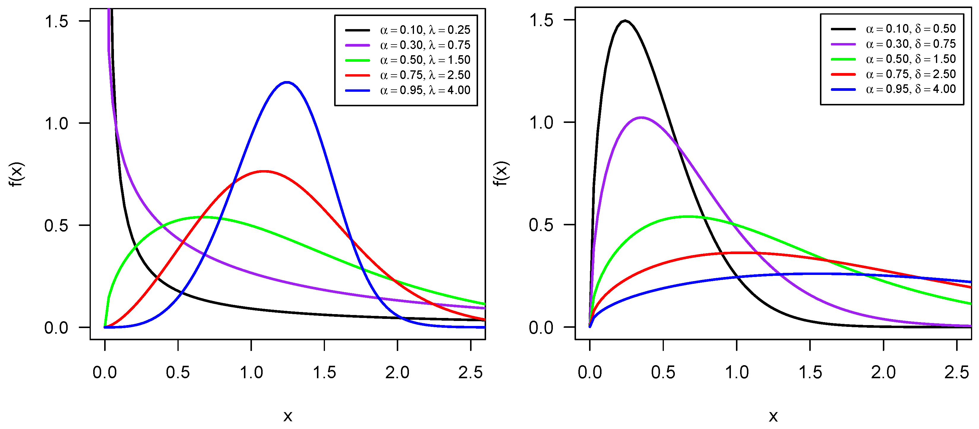
Figure 1.
The plots of PDF keeping constant (left) and (right).
Figure 1.
The plots of PDF keeping constant (left) and (right).
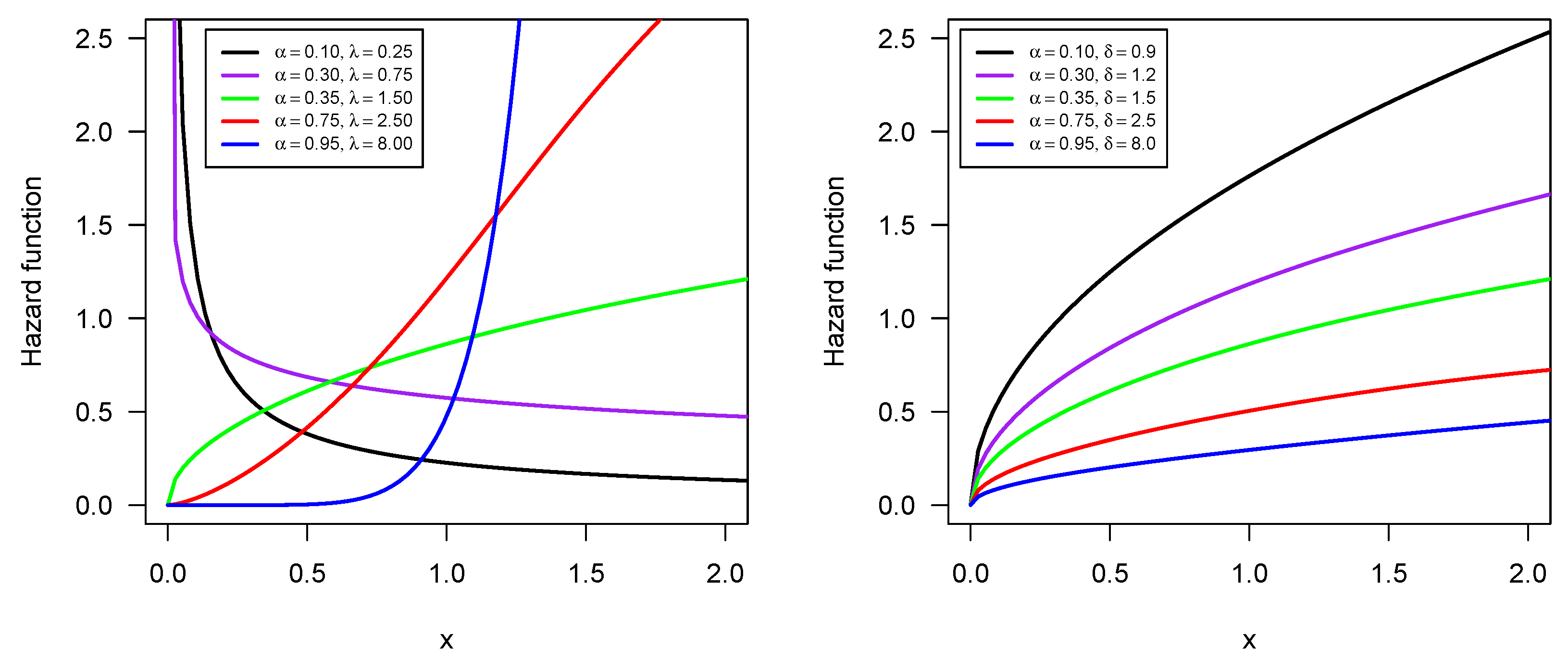
Figure 2.
The plots of HRF keeping constant (left) and (right).
Figure 2.
The plots of HRF keeping constant (left) and (right).
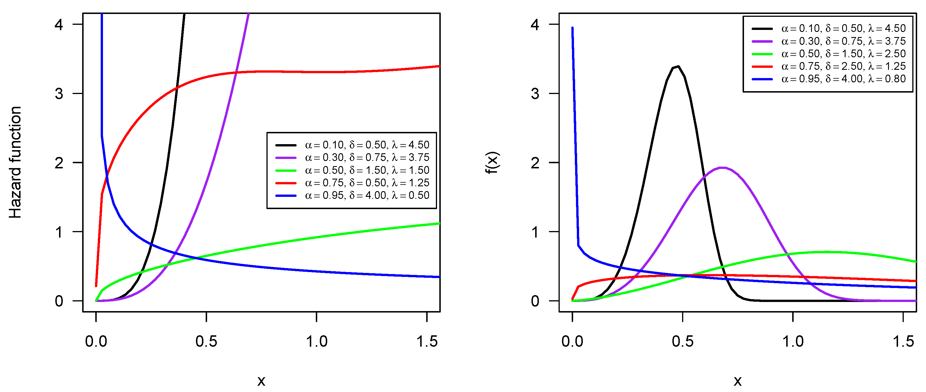
Figure 3.
The plots of PDF and HRF with a variation of all three parameters.
Figure 3.
The plots of PDF and HRF with a variation of all three parameters.
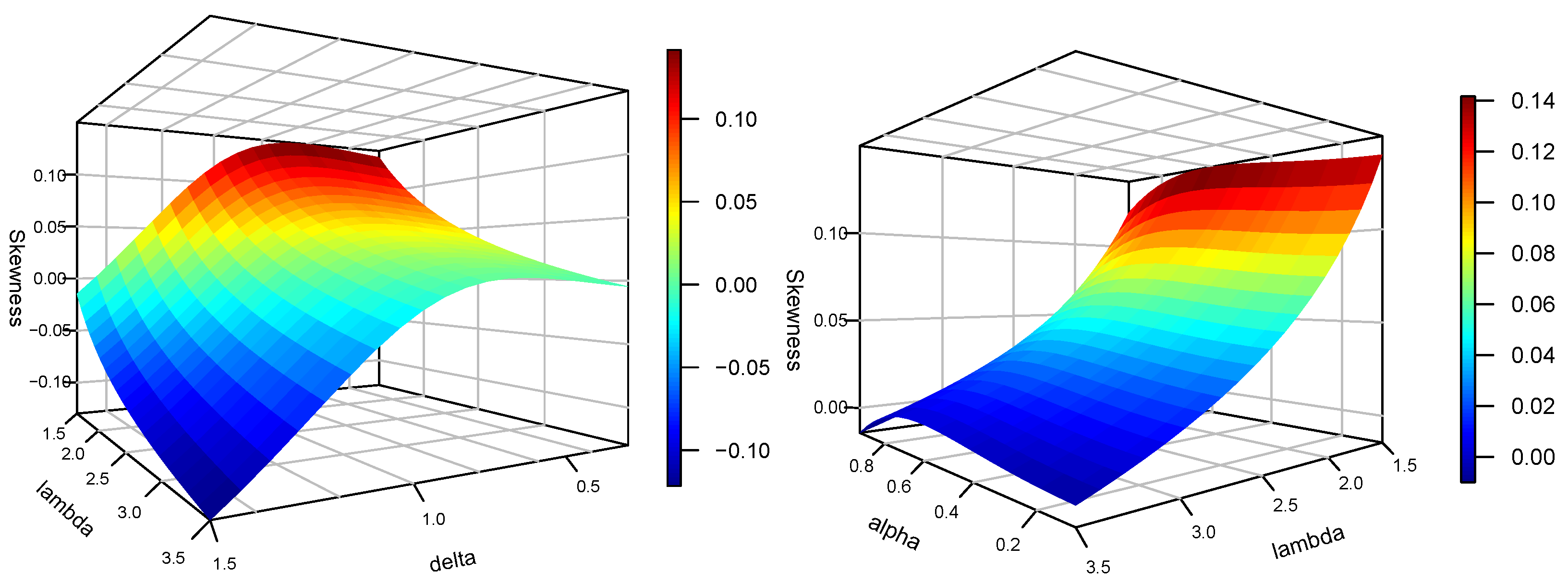
Figure 4.
The plots of skewness with constant (left) and constant (right).
Figure 4.
The plots of skewness with constant (left) and constant (right).
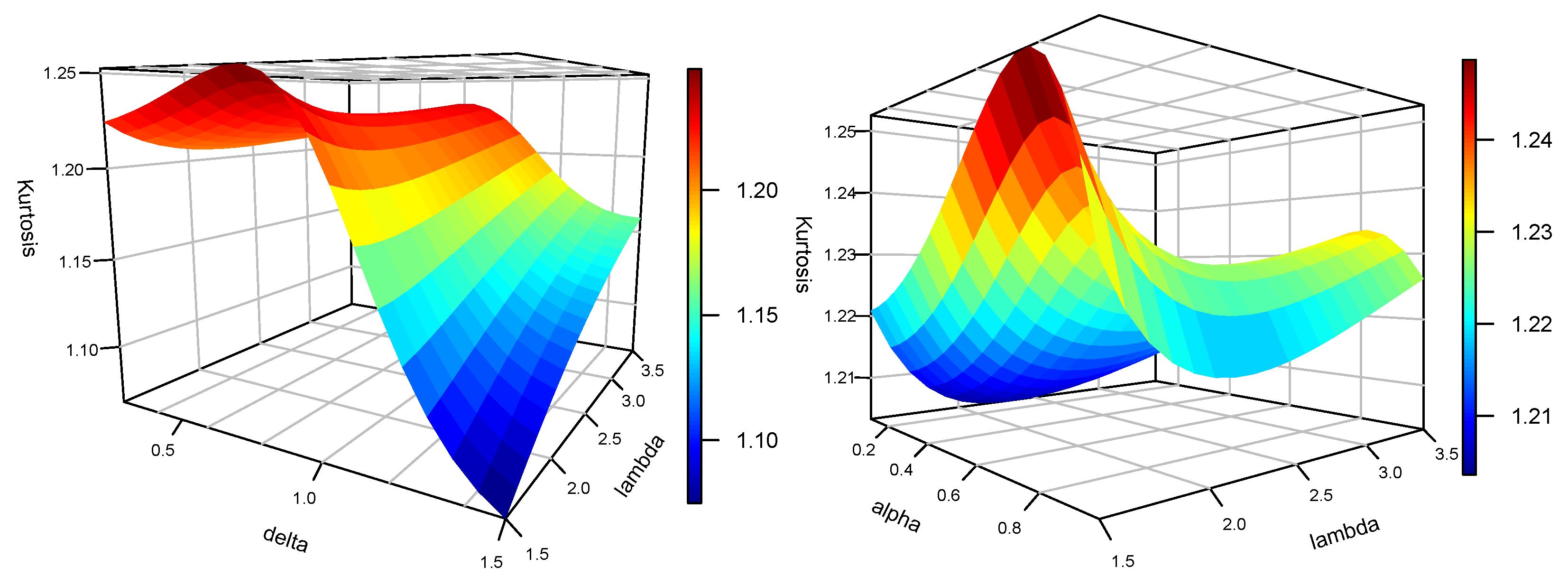
Figure 5.
The plots of kurtosis with constant (left) and constant (right).
Figure 5.
The plots of kurtosis with constant (left) and constant (right).
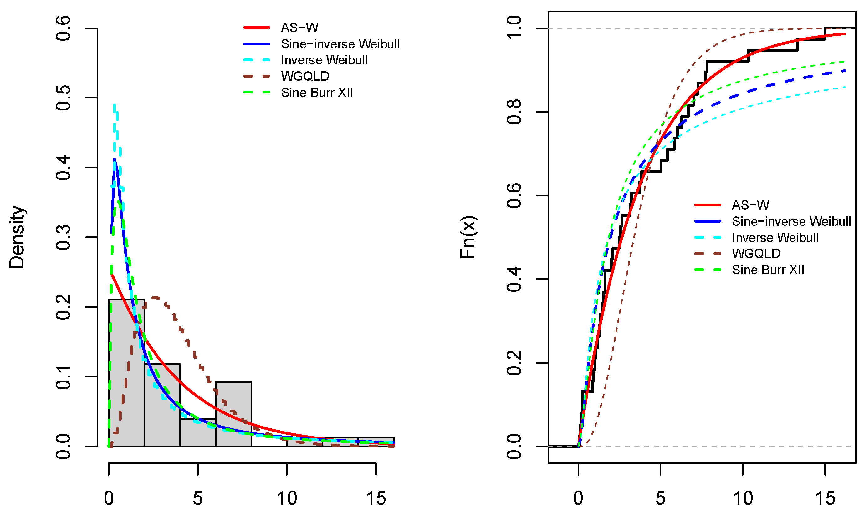
Figure 6.
Plots of estimated probability density functions and cumulative distribution functions for Dataset 1.
Figure 6.
Plots of estimated probability density functions and cumulative distribution functions for Dataset 1.
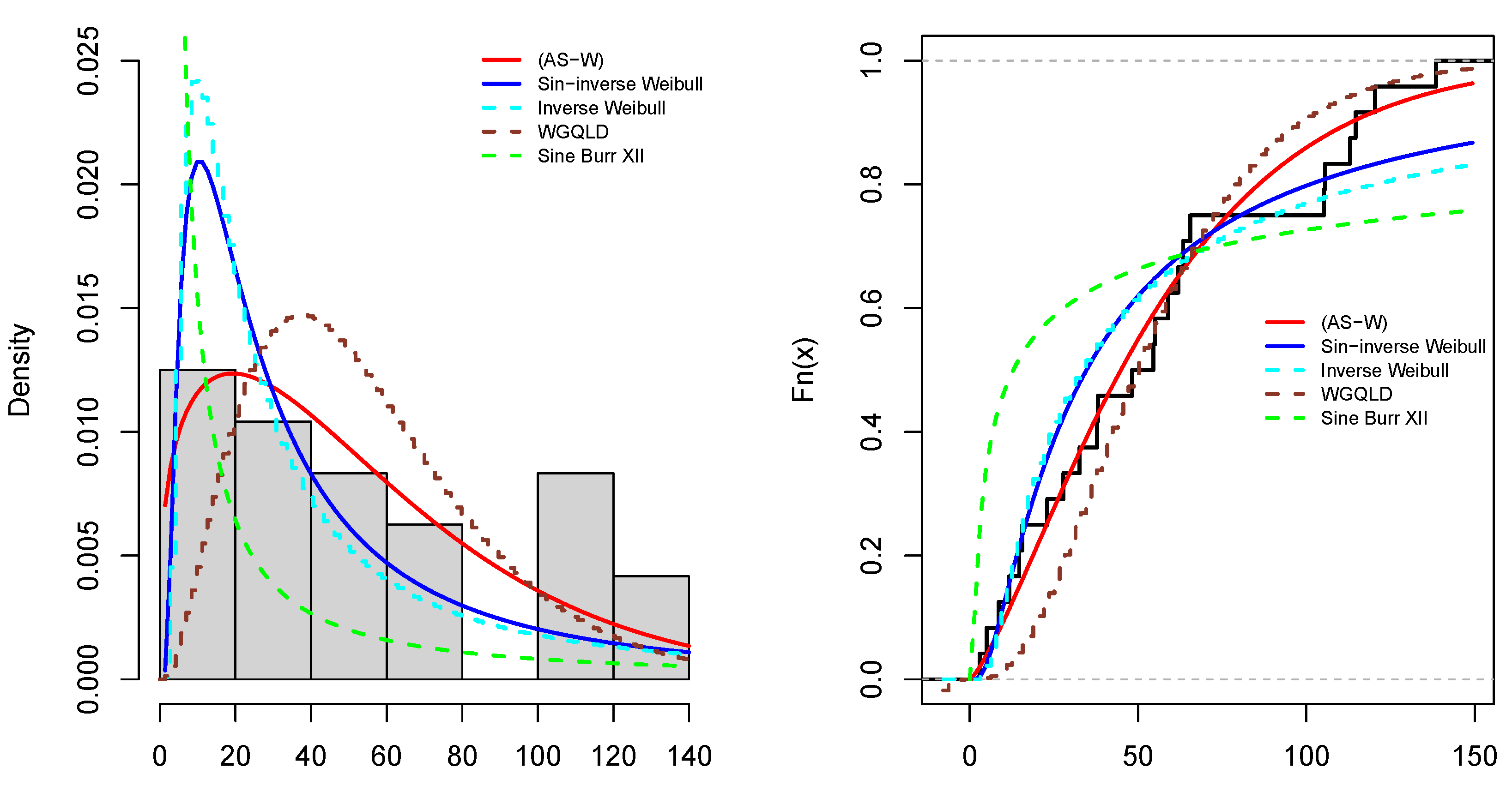
Figure 7.
Plots of estimated probability density functions and cumulative distribution functions for Dataset 2.
Figure 7.
Plots of estimated probability density functions and cumulative distribution functions for Dataset 2.
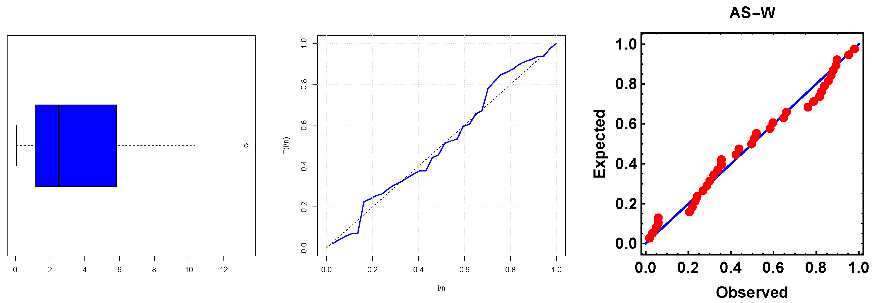
Figure 8.
Box, TTT, and PP plots for the first real data set.
Figure 8.
Box, TTT, and PP plots for the first real data set.
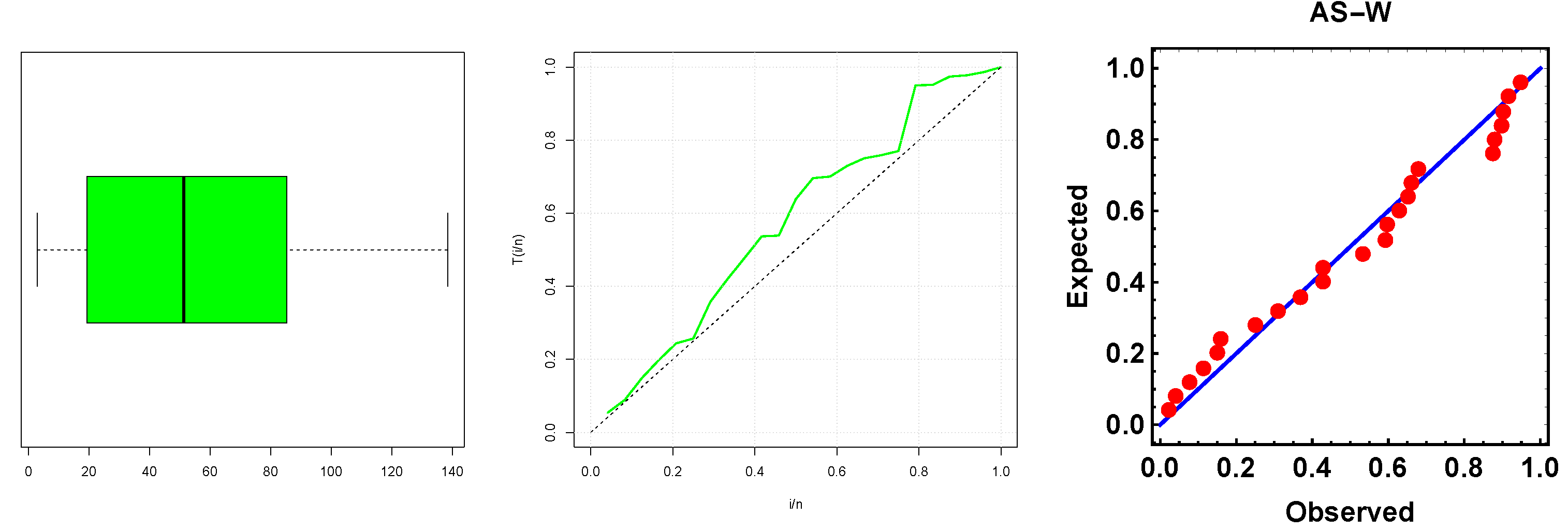
Figure 9.
Box, TTT, and PP plots for the second real data set.
Figure 9.
Box, TTT, and PP plots for the second real data set.
Table 1.
Various measures based on quantiles.
Table 1.
Various measures based on quantiles.
| Statistical Measure | Expression |
|---|
| Median | |
| Lower Quartile | |
| Upper Quartile | |
| QD | |
| Coefficient of QD | |
| Skewness [20] | |
| Kurtosis [21] | |
Table 2.
The AES and MSEs of .
Table 2.
The AES and MSEs of .
| Sample Size | | MLE | MPS | LSE | WLS | CVE | ADE |
|---|
| | AE | MSE | AE | MSE | AE | MSE | AE | MSE | AE | MSE | AE | MSE |
|---|
| 30 | | 0.4282 | 0.2229 | 0.5727 | 0.2056 | 0.4468 | 0.2089 | 0.4707 | 0.2165 | 0.3965 | 0.2279 | 0.4661 | 0.2144 |
| | | 2.0909 | 0.3833 | 2.2162 | 0.4673 | 2.1140 | 0.2179 | 2.1152 | 0.1477 | 2.0552 | 0.0475 | 2.1046 | 0.1377 |
| | | 3.1459 | 0.3697 | 2.7929 | 0.2730 | 2.9844 | 0.3670 | 3.0017 | 0.3144 | 3.2108 | 0.4036 | 3.0294 | 0.2770 |
| 60 | | 0.5516 | 0.0155 | 0.5333 | 0.1673 | 0.4501 | 0.1589 | 0.4570 | 0.1585 | 0.3957 | 0.1626 | 0.4503 | 0.1587 |
| | | 2.0105 | 0.0031 | 2.1136 | 0.0490 | 2.0668 | 0.0376 | 2.0637 | 0.0282 | 2.0285 | 0.0191 | 2.0594 | 0.0284 |
| | | 3.0861 | 0.0258 | 2.8456 | 0.1225 | 2.9515 | 0.1485 | 2.9718 | 0.1242 | 3.0802 | 0.1362 | 2.9820 | 0.1158 |
| 100 | | 0.5429 | 0.0129 | 0.5160 | 0.1593 | 0.4173 | 0.1547 | 0.4282 | 0.1496 | 0.3918 | 0.1458 | 0.4378 | 0.1519 |
| | | 2.0054 | 0.0016 | 2.0937 | 0.0366 | 2.0448 | 0.0194 | 2.0446 | 0.0189 | 2.0211 | 0.0134 | 2.0490 | 0.0206 |
| | | 3.0741 | 0.0222 | 2.8854 | 0.0665 | 2.9601 | 0.0819 | 2.9766 | 0.0678 | 3.0436 | 0.0701 | 2.9799 | 0.0655 |
| 150 | | 0.5333 | 0.0100 | 0.5197 | 0.1487 | 0.4428 | 0.1360 | 0.4476 | 0.1369 | 0.4175 | 0.1318 | 0.4463 | 0.1386 |
| | | 2.0021 | 0.0006 | 2.0819 | 0.0287 | 2.0388 | 0.0154 | 2.0411 | 0.0155 | 2.0230 | 0.0125 | 2.0409 | 0.0157 |
| | | 3.0633 | 0.0190 | 2.9047 | 0.0439 | 2.9641 | 0.0539 | 2.9732 | 0.0442 | 3.0188 | 0.0451 | 2.9764 | 0.0427 |
| 200 | | 0.5237 | 0.0071 | 0.5464 | 0.1465 | 0.4247 | 0.1372 | 0.4404 | 0.1344 | 0.4234 | 0.1303 | 0.4439 | 0.1322 |
| | | 2.0003 | 0.0001 | 2.0910 | 0.0290 | 2.0323 | 0.0129 | 2.0366 | 0.0137 | 2.0256 | 0.0121 | 2.0366 | 0.0135 |
| | | 3.0531 | 0.0159 | 2.9242 | 0.0342 | 2.9802 | 0.0411 | 2.9868 | 0.0325 | 3.0209 | 0.0342 | 2.9892 | 0.0327 |
| 500 | | 0.5027 | 0.0008 | 0.4988 | 0.1292 | 0.4153 | 0.1220 | 0.4110 | 0.1198 | 0.3952 | 0.1173 | 0.4115 | 0.1188 |
| | | 2.0000 | 0.0000 | 2.0624 | 0.0207 | 2.0232 | 0.0096 | 2.0205 | 0.0095 | 2.0122 | 0.0081 | 2.0200 | 0.0094 |
| | | 3.0297 | 0.0089 | 2.9533 | 0.0145 | 2.9794 | 0.0166 | 2.9861 | 0.0138 | 3.0008 | 0.0137 | 2.9871 | 0.0136 |
Table 3.
The AES and MSEs of .
Table 3.
The AES and MSEs of .
| Sample Size | | MLE | MPS | LSE | WLS | CVE | ADE |
|---|
| | AE | MSE | AE | MSE | AE | MSE | AE | MSE | AE | MSE | AE | MSE |
|---|
| 30 | | 0.2849 | 0.1535 | 0.4189 | 0.1723 | 0.3544 | 0.1660 | 0.3813 | 0.1785 | 0.3276 | 0.1644 | 0.3751 | 0.1642 |
| | | 1.0271 | 0.0322 | 1.1228 | 0.2186 | 1.0844 | 0.3253 | 1.0866 | 0.0735 | 1.0361 | 0.0235 | 1.0658 | 0.0312 |
| | | 1.5828 | 0.0631 | 1.4216 | 0.0535 | 1.4915 | 0.0732 | 1.5027 | 0.0642 | 1.6071 | 0.0870 | 1.5224 | 0.0585 |
| 60 | | 0.4456 | 0.0091 | 0.4559 | 0.1658 | 0.3692 | 0.1467 | 0.3912 | 0.1513 | 0.3620 | 0.1387 | 0.3953 | 0.1506 |
| | | 1.0211 | 0.0049 | 1.1065 | 0.0401 | 1.0575 | 0.0192 | 1.0652 | 0.0222 | 1.0406 | 0.0167 | 1.0647 | 0.0230 |
| | | 1.5492 | 0.0098 | 1.4396 | 0.0255 | 1.4911 | 0.0357 | 1.4999 | 0.0295 | 1.5527 | 0.0348 | 1.5045 | 0.0271 |
| 100 | | 0.4443 | 0.0066 | 0.4371 | 0.1590 | 0.3933 | 0.1348 | 0.3974 | 0.1376 | 0.3694 | 0.1267 | 0.4026 | 0.1380 |
| | | 1.0214 | 0.0032 | 1.0922 | 0.0333 | 1.0584 | 0.0173 | 1.0603 | 0.0187 | 1.0403 | 0.0139 | 1.0611 | 0.0192 |
| | | 1.5381 | 0.0057 | 1.4635 | 0.0143 | 1.4995 | 0.0197 | 1.5059 | 0.0160 | 1.5389 | 0.0182 | 1.5087 | 0.0157 |
| 150 | | 0.4456 | 0.0068 | 0.4645 | 0.1582 | 0.3779 | 0.1307 | 0.3865 | 0.1320 | 0.3649 | 0.1234 | 0.3895 | 0.1330 |
| | | 1.0136 | 0.0020 | 1.0971 | 0.0329 | 1.0486 | 0.0138 | 1.0509 | 0.0149 | 1.0363 | 0.0116 | 1.0520 | 0.0157 |
| | | 1.5297 | 0.0045 | 1.4626 | 0.0106 | 1.4918 | 0.0140 | 1.4976 | 0.0114 | 1.5198 | 0.0122 | 1.4988 | 0.0110 |
| 200 | | 0.4410 | 0.0061 | 0.4412 | 0.1528 | 0.3754 | 0.1280 | 0.3748 | 0.1271 | 0.3583 | 0.1200 | 0.3764 | 0.1296 |
| | | 1.0118 | 0.0018 | 1.0898 | 0.0296 | 1.0505 | 0.0129 | 1.0492 | 0.0137 | 1.0379 | 0.0111 | 1.0508 | 0.0146 |
| | | 1.5245 | 0.0037 | 1.4695 | 0.0080 | 1.4901 | 0.0101 | 1.4969 | 0.0082 | 1.5137 | 0.0086 | 1.4972 | 0.0080 |
| 500 | | 0.4380 | 0.0057 | 0.4484 | 0.1420 | 0.3764 | 0.1161 | 0.3778 | 0.1151 | 0.3629 | 0.1094 | 0.3789 | 0.1153 |
| | | 1.0012 | 0.0002 | 1.0815 | 0.0264 | 1.0413 | 0.0110 | 1.0416 | 0.0121 | 1.0330 | 0.0098 | 1.0418 | 0.0122 |
| | | 1.5115 | 0.0017 | 1.4802 | 0.0034 | 1.4932 | 0.0039 | 1.4960 | 0.0032 | 1.5034 | 0.0032 | 1.4964 | 0.0032 |
Table 4.
The AES and MSEs of .
Table 4.
The AES and MSEs of .
| Sample Size | | MLE | MPS | LSE | WLS | CVE | ADE |
|---|
| | AE | MSE | AE | MSE | AE | MSE | AE | MSE | AE | MSE | AE | MSE |
|---|
| 30 | | 0.6597 | 0.0195 | 0.5390 | 0.2054 | 0.5081 | 0.1784 | 0.5212 | 0.1858 | 0.4882 | 0.1821 | 0.5191 | 0.1895 |
| | | 2.0642 | 0.1340 | 2.6170 | 8.4422 | 2.3168 | 2.3140 | 2.3242 | 1.8946 | 2.2091 | 2.7088 | 2.2942 | 1.1570 |
| | | 1.0537 | 0.0140 | 0.9369 | 0.0276 | 0.9900 | 0.0380 | 0.9979 | 0.0330 | 1.0665 | 0.0433 | 1.0081 | 0.0285 |
| 60 | | 0.6494 | 0.0099 | 0.5570 | 0.1611 | 0.4988 | 0.1622 | 0.5099 | 0.1605 | 0.4692 | 0.1636 | 0.5016 | 0.1645 |
| | | 2.0634 | 0.0127 | 2.2948 | 0.4264 | 2.1652 | 0.3995 | 2.1645 | 0.2667 | 2.0678 | 0.1926 | 2.1487 | 0.2479 |
| | | 1.0276 | 0.0055 | 0.9435 | 0.0135 | 0.9803 | 0.0164 | 0.9865 | 0.0139 | 1.0219 | 0.0152 | 0.9883 | 0.0125 |
| 100 | | 0.6442 | 0.0088 | 0.5808 | 0.1450 | 0.5099 | 0.1456 | 0.5104 | 0.1474 | 0.4700 | 0.1500 | 0.5034 | 0.1487 |
| | | 2.0510 | 0.0102 | 2.2622 | 0.3124 | 2.1219 | 0.2023 | 2.1178 | 0.1835 | 2.0400 | 0.1417 | 2.1039 | 0.1735 |
| | | 1.0250 | 0.0050 | 0.9625 | 0.0075 | 0.9858 | 0.0086 | 0.9913 | 0.0073 | 1.0135 | 0.0078 | 0.9944 | 0.0070 |
| 150 | | 0.6378 | 0.0076 | 0.5631 | 0.1385 | 0.4894 | 0.1464 | 0.4867 | 0.1480 | 0.4572 | 0.1500 | 0.4871 | 0.1483 |
| | | 2.0552 | 0.0110 | 2.2113 | 0.2558 | 2.0807 | 0.1505 | 2.0728 | 0.1324 | 2.0186 | 0.1090 | 2.0729 | 0.1341 |
| | | 1.0140 | 0.0028 | 0.9649 | 0.0054 | 0.9829 | 0.0063 | 0.9873 | 0.0051 | 1.0024 | 0.0051 | 0.9883 | 0.0050 |
| 200 | | 0.6272 | 0.0054 | 0.5662 | 0.1418 | 0.4872 | 0.1449 | 0.4817 | 0.1453 | 0.4546 | 0.1477 | 0.4877 | 0.1450 |
| | | 2.0500 | 0.0100 | 2.2230 | 0.2529 | 2.0804 | 0.1423 | 2.0684 | 0.1301 | 2.0218 | 0.1096 | 2.0768 | 0.1367 |
| | | 1.0108 | 0.0022 | 0.9718 | 0.0041 | 0.9895 | 0.0048 | 0.9929 | 0.0039 | 1.0045 | 0.0040 | 0.9931 | 0.0038 |
| 500 | | 0.608 | 0.0016 | 0.5878 | 0.1189 | 0.4732 | 0.1353 | 0.4847 | 0.1241 | 0.4688 | 0.1234 | 0.4885 | 0.1239 |
| | | 2.000 | 0.0000 | 2.2199 | 0.2269 | 2.0446 | 0.0999 | 2.0459 | 0.0965 | 2.0175 | 0.0843 | 2.0511 | 0.1001 |
| | | 1.000 | 0.0000 | 0.9808 | 0.0018 | 0.9936 | 0.0018 | 0.9949 | 0.0015 | 1.0000 | 0.0015 | 0.9949 | 0.0015 |
Table 5.
The AES and MSEs of .
Table 5.
The AES and MSEs of .
| Sample Size | | MLE | MPS | LSE | WLS | CVE | ADE |
|---|
| | AE | MSE | AE | MSE | AE | MSE | AE | MSE | AE | MSE | AE | MSE |
|---|
| 30 | | 0.7483 | 0.0274 | 0.7345 | 0.1700 | 0.6787 | 0.1822 | 0.6691 | 0.1730 | 0.5878 | 0.2083 | 0.6681 | 0.1844 |
| | | 3.0782 | 0.0368 | 3.5572 | 3.0963 | 3.4365 | 2.7615 | 3.3212 | 1.4609 | 3.1723 | 0.7521 | 3.3279 | 1.4390 |
| | | 2.5959 | 0.0441 | 2.2631 | 0.2335 | 2.4062 | 0.2695 | 2.4325 | 0.2375 | 2.6046 | 0.2761 | 2.4583 | 0.2202 |
| 60 | | 0.7210 | 0.0063 | 0.6983 | 0.1259 | 0.6762 | 0.1393 | 0.6420 | 0.1358 | 0.5789 | 0.1566 | 0.6587 | 0.1363 |
| | | 3.0507 | 0.0152 | 3.2034 | 0.1991 | 3.1919 | 0.3088 | 3.1130 | 0.1402 | 3.0399 | 0.1163 | 3.1341 | 0.1548 |
| | | 2.5813 | 0.0244 | 2.3468 | 0.1024 | 2.4330 | 0.1317 | 2.4604 | 0.1028 | 2.5513 | 0.1109 | 2.4620 | 0.0987 |
| 100 | | 0.7054 | 0.0016 | 0.6886 | 0.1179 | 0.6692 | 0.1197 | 0.6293 | 0.1264 | 0.5736 | 0.1445 | 0.6494 | 0.1217 |
| | | 3.0354 | 0.0106 | 3.1517 | 0.1021 | 3.1244 | 0.1366 | 3.0739 | 0.0787 | 3.0172 | 0.0689 | 3.0901 | 0.0833 |
| | | 2.5756 | 0.0227 | 2.3837 | 0.0631 | 2.4531 | 0.0757 | 2.4717 | 0.0618 | 2.5291 | 0.0638 | 2.4711 | 0.0590 |
| 150 | | 0.7027 | 0.0008 | 0.6884 | 0.1119 | 0.6650 | 0.1186 | 0.6020 | 0.1345 | 0.5654 | 0.1444 | 0.6330 | 0.1253 |
| | | 3.0246 | 0.0074 | 3.1333 | 0.0846 | 3.1112 | 0.1146 | 3.0444 | 0.0621 | 3.0061 | 0.0571 | 3.0696 | 0.0679 |
| | | 2.5552 | 0.0166 | 2.3985 | 0.0393 | 2.4481 | 0.0500 | 2.4685 | 0.0377 | 2.5075 | 0.0375 | 2.4649 | 0.0371 |
| 200 | | 0.7006 | 0.0002 | 0.6686 | 0.1123 | 0.6532 | 0.1147 | 0.5924 | 0.1309 | 0.5587 | 0.1392 | 0.6294 | 0.1191 |
| | | 3.0168 | 0.0050 | 3.1048 | 0.0724 | 3.0849 | 0.0863 | 3.0256 | 0.0514 | 2.9926 | 0.0492 | 3.0551 | 0.0578 |
| | | 2.5450 | 0.0135 | 2.4154 | 0.0282 | 2.4574 | 0.0366 | 2.4756 | 0.0275 | 2.5059 | 0.0279 | 2.4706 | 0.0272 |
| 500 | | 0.7000 | 0.0000 | 0.6829 | 0.0887 | 0.6505 | 0.0995 | 0.5927 | 0.1110 | 0.5671 | 0.1176 | 0.6345 | 0.0976 |
| | | 3.0000 | 0.0000 | 3.0887 | 0.0561 | 3.0578 | 0.0586 | 3.0039 | 0.0359 | 2.9809 | 0.0339 | 3.0369 | 0.0428 |
| | | 2.5126 | 0.0038 | 2.4351 | 0.0132 | 2.4620 | 0.0144 | 2.4740 | 0.0107 | 2.4876 | 0.0101 | 2.4687 | 0.0112 |
Table 6.
Summary statistics for the selected datasets.
Table 6.
Summary statistics for the selected datasets.
| Datasets | Minimum | One Quntile | Median | Mean | Three Quntile | Maximum | Skew | Kurt |
|---|
| Dataset 1 | 0.070 | 1.170 | 2.490 | 3.494 | 5.840 | 13.300 | 1.152 | 3.890 |
| Dataset 2 | 2.998 | 21.187 | 51.385 | 55.123 | 75.435 | 138.500 | 0.555 | 2.108 |
Table 7.
The total annual rainfall.
Table 7.
The total annual rainfall.
| 1.33 | 1.43 | 1.01 | 1.62 | 3.15 | 1.05 | 7.72 | 0.2 | 6.03 | 0.25 | 7.83 | 0.25 | 0.88 | 6.29 | 0.94 |
| 5.84 | 3.23 | 3.7 | 1.26 | 2.64 | 1.17 | 2.49 | 1.62 | 2.1 | 0.14 | 2.57 | 3.85 | 7.02 | 5.04 | 7.27 |
| 1.53 | 6.7 | 0.07 | 2.01 | 10.35 | 5.42 | 13.3 | | | | | | | | |
Table 8.
The values of the failure times of eight components at three different temperatures.
Table 8.
The values of the failure times of eight components at three different temperatures.
| 14.712 | 32.644 | 61.979 | 65.521 | 105.50 | 114.60 | 120.40 |
| 138.50 | 8.610 | 11.741 | 54.535 | 55.047 | 58.928 | 63.391 |
| 105.18 | 113.02 | 2.998 | 5.016 | 15.628 | 23.040 | 27.851 |
| 37.843 | 38.050 | 48.226 | | | | |
Table 9.
The MLEs, SEs and corresponding log-likelihood values for the AS-G FD model.
Table 9.
The MLEs, SEs and corresponding log-likelihood values for the AS-G FD model.
| Datasets | Estimate | SE | |
|---|
| Dataset 1 | = 0.0003 | 1.1977 | −83.265 |
| | = 1.0495 | 0.1381 | |
| | = 3.55905 | 0.5862 | |
| Dataset 2 | = 0.002 | 1.083 | −119.119 |
| | = 59.518 | 9.820 | |
| | = 1.300 | 0.216 | |
Table 10.
The goodness of fit tests for Dataset 1.
Table 10.
The goodness of fit tests for Dataset 1.
| Model | AIC | AICc | BIC | HQIC | K-S | p-Value |
|---|
| AS-W | 172.5304 | 173.2577 | 177.3632 | 174.2342 | 0.0907 | 0.9212 |
| Sine-inverse Weibull | 184.3137 | 184.6666 | 187.5355 | 185.4495 | 0.15862 | 0.3096 |
| Inverse Weibull | 190.8537 | 191.2066 | 194.0755 | 191.9896 | 0.1897 | 0.1394 |
| WGQLD | 206.7907 | 207.1436 | 210.0125 | 207.9265 | 0.2682 | 0.0097 |
| Sine Burr XII | 181.3963 | 181.7493 | 184.6181 | 182.5322 | 0.1423 | 0.4417 |
Table 11.
The goodness of fit tests for Dataset 2.
Table 11.
The goodness of fit tests for Dataset 2.
| Model | AIC | AICc | BIC | HQIC | K-S | p-Value |
|---|
| AS-W | 244.239 | 245.439 | 247.7732 | 245.1767 | 0.1271 | 0.7875 |
| Sine-inverse Weibull | 251.187 | 251.7585 | 253.5431 | 251.8121 | 0.1546 | 0.5622 |
| Inverse Weibull | 255.0592 | 255.6306 | 257.4153 | 255.6843 | 0.1778 | 0.3884 |
| WGQLD | 252.8124 | 253.3839 | 255.1686 | 253.4375 | 0.1950 | 0.2824 |
| Sine Burr XII | 284.8518 | 285.4232 | 287.2079 | 285.4768 | 0.3609 | 0.0026 |


 ,
, 


