Thermal–Structural Linear Static Analysis of Functionally Graded Beams Using Reddy Beam Theory

Abstract

In this work, a finite element model to perform the thermal–structural analysis of beams made of functionally graded material (FGM) is presented. The formulation is based on the third-order shear deformation theory. The constituents of the FGM are considered to vary only in the thickness direction, and the effective material properties are evaluated by means of the rule of mixtures. The volume distribution of the top constituent is modeled using the power law form. A comparison of the present finite element model with the numerical results available in the literature reveals that they are in good agreement. In addition, a routine to study functionally graded plane models in a commercial finite element code is used to verify the performance of the proposed model. In the present work, displacements for different values of the power law exponent and surface temperatures are presented. Furthermore, the normal stress variation along the thickness is shown for several power law exponents of functionally graded beams subjected to thermal and mechanical loads.

1. Introduction

Functionally graded materials (FGMs) are advanced materials made from a mixture of two or more constituents, and, therefore, they are not homogeneous. Typically, the mixture consists of a ceramic and a metallic material, and it is designed to have a continuous variation in material composition. The gradient of material properties allows the reduction of thermal and residual stresses, as well as the stress concentrations presented in laminated composite materials [1,2,3,4,5].

FGMs are often used in structures or applications that commonly operate under extreme temperature and/or environmental conditions, such as spacecrafts, aircrafts, and nuclear reactors [6,7,8]. The main reasons for their use are their outstanding thermo-mechanical properties, corrosion resistance, and high fracture toughness [9].

Many of the structural elements or components operating under these extreme environments are beams. For that reason, it is important to analyze the behavior of these types of elements [6]. Since the beam element is one of the most used in structural analysis, there are several theories available to describe its mechanical behavior. Among these are Euler–Bernoulli beam theory or classical beam theory (CBT), Timoshenko beam theory or first-order shear deformation theory (FSDT), Reddy–Bickford beam theory or third-order shear deformation theory (TSDT), and other higher-order shear deformation theories (HSDTs).

Static, dynamic, and modal analyses of functionally graded beams under mechanical loads have been made using these theories. Li [10] presented a unified approach to analyze the static and dynamic behavior of functionally graded beams (FGB), where the Euler–Bernoulli beam theory could be reduced from the Timoshenko beam theory as a special case. Alshorbagy et al. [11] investigated the free vibration response of FGB by means of the finite element method and the CBT. Moheimani and Ahmadian [12] studied the free vibration response of FGB using the Euler–Bernoulli beam theory and the non-local theory of elasticity. Chakraborty et al. [1] performed static and free vibration analyses of FGB using the FSDT. Nguyen et al. [13] studied the static and free vibration responses of axially loaded rectangular FGB using the FSDT. A higher-order finite element, based on the unified and integrated approach of Timoshenko beam theory, was developed by Katili et al. [14]. They performed static and free vibration analyses of FGB. Kadoli et al. [15] presented the static analysis of FGB using the TSDT. The free vibration of FGB was investigated by Aydogdu and Taskin [16] by means of a Navier-type solution method and different higher-order shear deformation theories. Mahi et al. [17] developed an exact model to study the free vibration response of FGB using a unified HSDT, where the material properties were taken as temperature-dependent. Thai and Vo [18] used different HSDTs to study the bending and free vibration of FGB. A similar analysis was made later by Vo et al. [19] using only a refined shear deformation theory. Şimşek and Reddy [20] studied the static bending and free vibration of functionally graded (FG) microbeams using a unified higher-order theory that contained various other theories by introducing a function into the displacement field that characterized the transverse shear and stress distribution along the thickness of the beam. Gao and Zhang [21] developed a non-classical third-order shear deformation beam theory for Reddy–Levinson beams using a modified couple stress theory and a surface elasticity theory that allowed them to consider the beam’s microstructure, surface energy, and Poisson’s effect.

The responses of functionally graded beams under thermal and mechanical loads have also been explored. Chakraborty and Gopalakrishnan [22] analyzed the wave propagation behavior of FGB subjected to high-frequency thermal or mechanical impulses using the spectral finite element method. Daneshmehr et al. [23] developed a micro-scale Reddy beam model based on the couple stress theory to analyze the thermal effect on the vibration, buckling, and static bending analyses. They obtained solutions using series expansions for the generalized displacements, which satisfied the boundary conditions. El-Megharbel [9] performed a theoretical analysis of FGB under thermal loads. De Pietro et al. [7] studied the thermo-elastic response of FGB using Carrera’s unified formulation. Lim and Kim [24] used the FSDT to analyze the behavior of FGB with temperature-dependent material properties. Ebrahimi and Jafari [3] proposed a refined shear deformation beam theory for the thermo-mechanical analysis of FGB with porosities exposed to different thermal loads.

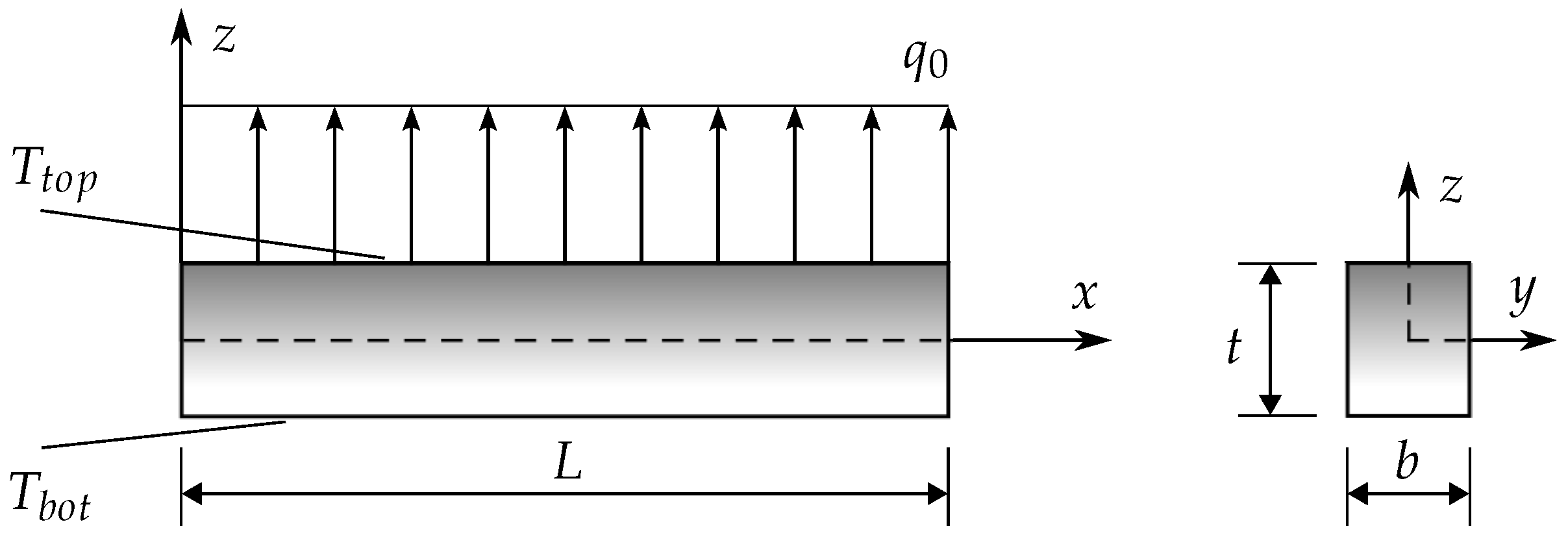
In this paper, a thermal-structural analysis of FGB is presented. The finite element model is developed using the TSDT. The material properties vary through the thickness according to the power law, and the temperature distribution along the same direction is obtained by means of a polynomial series. To verify the behavior of the present finite element model, plane models are developed using ANSYS APDL. Finally, to illustrate the performance of the model, some case studies are reported, where the power law exponent and the difference in the temperature between the top and bottom surfaces are varied.

2. Thermal–Structural Problem Description

To develop the present finite element model of FG beams under thermal and mechanical loads, the following conditions are considered:

• The FG beam has a rectangular cross-section of width b and thickness t, as shown in Figure 1, and the beam’s length is L.
• The top and bottom surfaces, as seen in Figure 1, are exposed to the temperatures $T_{top}$ and $T_{bot}$, respectively, where $T_{top}>T_{bot}$. The temperature only varies through the z coordinate, and it remains constant along the other directions.
• There is no internal heat generation, and convection heat transfer between the beam’s surfaces and the surrounding media is not considered.
• In this case, a uniform distributed load $q_0$ is applied to the FG beam, as shown in Figure 1. However, the distributed load can also be function of the x coordinate.

2.1. Mechanical Properties

In order to model the variation in the mechanical properties with the variation in the thickness of the beam, Voight’s rule of mixtures is used [25], as follows:

$$P\left(z\right)=\left(P_{top}-P_{bot}\right)V_{top}\left(z\right)+P_{bot},$$

(1)

where P denotes the material property and the subscripts $top$ and $bot$ refer to the top and bottom constituent, respectively. $V_{top}\left(z\right)$ corresponds to the volume distribution of the top constituent through the thickness of the beam, which is defined by the power law as

$$V_{top}\left(z\right)={\left({\displaystyle \frac{2z+t}{2t}}\right)}^n,$$

(2)

where n is the power law exponent, which takes positive values.

2.2. Temperature Distribution

Following the assumptions stated in the problem description of Section 2, the governing equation of the heat transfer through the thickness of the beam is given by

$${\displaystyle \frac{\partial }{\partial z}}\left[K\left(z\right){\displaystyle \frac{\partial T\left(z\right)}{\partial z}}\right]=0,-t/2\le z\le t/2,$$

(3)

where $K\left(z\right)$ corresponds to the thermal conductivity, and it is calculated using Equation (1). In addition, the boundary conditions are

$$\begin{array}{cc}T(-t/2)=T_{bot},& T(t/2)=T_{top}.\end{array}$$

A solution to the above one-dimensional heat transfer equation was reported in the work of Javaheri and Eslami [26], and it is given as

$${\displaystyle T\left(z\right)=T_{bot}+{\displaystyle \frac{T_{top}-T_{bot}}{H}}\sum _{i=0}^{\eta }\left({\displaystyle \frac{1}{in+1}}\right){\left({\displaystyle \frac{K_{bot}-K_{top}}{K_{bot}}}\right)}^i{\left({\displaystyle \frac{2z+t}{2t}}\right)}^{\left(in+1\right)},}$$

(4)

with

$$H=\sum _{i=0}^{\eta }\left({\displaystyle \frac{1}{in+1}}\right){\left({\displaystyle \frac{K_{bot}-K_{top}}{K_{bot}}}\right)}^i,$$

where i indicates the index of the sum and $\eta$ denotes the number of terms used in the series for the approximation. One should also remember that n corresponds to the power law exponent presented previously in Equation (2).

3. Finite Element Model

This section briefly presents the development of the finite element model based on the TSDT. In order to obtain the equations for the present model (i.e., the stiffness matrix and generalized force vector), the definitions for the displacement field, strains, and constitutive equations are required. The displacement field of the TSDT is given by [27,28]

$$u_1\left(x\right) = u^0\left(x\right)+z{\varphi }^0\left(x\right)-\kappa z^3\left[{\varphi }^0\left(x\right)+{\displaystyle \frac{\partial w^0\left(x\right)}{\partial x}}\right],$$

(5)

$$u_3\left(x\right) = w^0\left(x\right),$$

(6)

where $u^0$ is the axial displacement, $w^0$ is the transverse displacement, ${\varphi }^0$ is the rotation of a point located at the centroidal axis x of the beam, and

$$\kappa =\frac{4}{3t^2}.$$

(7)

Considering the displacement field of Equations (5) and (6), the nonzero mechanical strains are defined as follows:

$${\epsilon }_{11}^{\mathrm{M}} = {\displaystyle \frac{\partial u^0}{\partial x}}+z{\displaystyle \frac{\partial {\varphi }^0}{\partial x}}-\kappa z^3\left({\displaystyle \frac{\partial {\varphi }^0}{\partial x}}+{\displaystyle \frac{{\partial }^2{w}^0}{\partial x^2}}\right)$$

(8)

$${\gamma }_{13}^{\mathrm{M}} = {\varphi }^0-3\kappa z^2\left({\varphi }^0+{\displaystyle \frac{\partial w^0}{\partial x}}\right)+{\displaystyle \frac{\partial w^0}{\partial x}}.$$

(9)

where, for the sake of brevity, the x argument has been omitted and the superscript M stands for mechanical. On the other hand, the nonzero thermal strain is defined as

$${\epsilon }_{11}^T=\alpha \left(z\right)\left[T\left(z\right)-T_{ref}\right],$$

(10)

where $\alpha \left(z\right)$ denotes the thermal expansion coefficient, and its value is computed by means of the rule of mixtures defined in Equation (1). $T\left(z\right)$ is calculated using Equation (4), $T_{ref}$ is the reference temperature at which the material is free of stress, and the superscript T stands for thermal.

Now, the constitutive equations are defined, i.e., the relation between stress and strain. In this case, the stresses, including thermal and mechanical effects, are considered to be defined by

$${\sigma }_{11}={\sigma }_{11}^M-{\sigma }_{11}^T,{\tau }_{13}={\tau }_{13}^M,$$

(11)

where

$${\sigma }_{11}^M=E\left(z\right){\epsilon }_{11}^M,{\sigma }_{11}^T=E\left(z\right){\epsilon }_{11}^T,{\tau }_{13}^M=G\left(z\right){\gamma }_{13}^M,$$

(12)

where $E\left(z\right)$ represents Young’s modulus and $G\left(z\right)$ is the shear modulus, which is defined as $G\left(z\right)={\displaystyle \frac{E\left(z\right)}{2\left(1+\nu \left(z\right)\right)}}$, where $\nu \left(z\right)$ is Poisson’s ratio.

3.1. Principle of Virtual Work

Here, to obtain the stiffness matrix and the force vector involved in the finite element model, the following definition of the principle of virtual work is used:

$$\delta W_I-\delta W_E=0,$$

(13)

where $\delta W_I$ is the virtual work carried out by internal forces and $\delta W_E$ is the virtual work carried out by external forces, which are defined by the following expressions:

$$\begin{array}{cc}\delta W_I={\int }_V\delta \epsilon ·\sigma dV,& \delta W_E={\int }_{h^e}\mathbf{f}·\delta \mathbf{u}dx,\end{array}$$

(14)

where $\mathbf{f}$ represents the vector associated with the external loads.

For the present model, introducing the strains and stresses defined in Equations (8)–(11) into Equation (14), the following expressions for the virtual works are found:

$$\delta W_I={\int }_V\left[\delta {\epsilon }_{11}^{M}E\left(z\right){\epsilon }_{11}^M+\delta {\gamma }_{13}^{M}G\left(z\right){\gamma }_{13}^M-\delta {\epsilon }_{11}^{M}E\left(z\right){\epsilon }_{11}^T\right]dV,$$

(15)

and

$$\delta W_E={\int }_{h^e}{q}_0\delta w^0\left(x\right)dx,$$

(16)

where $h^e$ represents the one-dimensional domain of the element.

At this point, all the definitions required to obtain the equations involved in the finite element model have been introduced. In the following sections, the displacement vector, the stiffness matrix, and the generalized force vector are obtained.

3.2. Displacement Vector

In order to obtain the finite element model, the displacement field is approximated as follows:

$$\begin{array}{ccc}{\displaystyle u_j^0=\sum _{j=0}^p{\psi }_j^u{\Delta }_j^{\left(1\right)},}\hfill & {\displaystyle w_J^0=\sum _{J=0}^m{\psi }_J^w{\Delta }_J^{\left(2\right)},}\hfill & {\displaystyle {\varphi }_k^0=\sum _{k=0}^p{\psi }_k^{\varphi }{\Delta }_k^{\left(3\right)},}\hfill \end{array}$$

(17)

where the functions ${\psi }_j^u$ and ${\psi }_k^{\varphi }$ correspond to the linear Lagrange polynomials and the function ${\psi }_J^w$ represents the Hermite cubic interpolation functions. Moreover, ${\Delta }_j^{\left(1\right)}$, ${\Delta }_J^{\left(2\right)}$, and ${\Delta }_k^{\left(3\right)}$ are nodal displacements associated with axial displacement, transverse displacement, and rotation, respectively. In this manner, the displacement vector of the finite element model has the form

$$\Delta ={\left[\begin{array}{ccc}{\Delta }^{\left(1\right)}\hfill & {\Delta }^{\left(2\right)}\hfill & {\Delta }^{\left(3\right)}\hfill \end{array}\right]}^{\mathrm{T}}.$$

(18)

3.3. Stiffness Matrix and Generalized Force Vector

Substituting the strains and stresses into Equation (15) and then replacing the displacements by their approximations defined by Equation (17), the stiffness matrix is found to have the form

$${\mathbf{K}}^{\mathbf{e}}=\left[\begin{array}{ccc}{\mathbf{K}}^{11}& {\mathbf{K}}^{12}& {\mathbf{K}}^{13}\\ {\mathbf{K}}^{21}& {\mathbf{K}}^{22}& {\mathbf{K}}^{23}\\ {\mathbf{K}}^{31}& {\mathbf{K}}^{32}& {\mathbf{K}}^{33}\end{array}\right],$$

(19)

where the components of the submatrices ${\mathbf{K}}^{ij}$ are given by

$$\begin{array}{ccc}{\displaystyle K_{ij}^{11}={\int }_{h^e}{A}_{xx}{\displaystyle \frac{{\displaystyle d{\psi }_i^u}}{dx}}{\displaystyle \frac{{\displaystyle d{\psi }_j^u}}{dx}}dx,}\hfill & {\displaystyle K_{iJ}^{12}={\int }_{h^e}-\kappa E_{xx}{\displaystyle \frac{{\displaystyle d{\psi }_i^u}}{dx}}{\displaystyle \frac{{\displaystyle d^2{\psi }_J^w}}{d{x}^2}}dx,}\hfill & {\displaystyle K_{il}^{13}={\int }_{h^e}{\widehat{B}}_{xx}{\displaystyle \frac{{\displaystyle d{\psi }_i^u}}{dx}}{\displaystyle \frac{{\displaystyle d{\psi }_l^{\varphi }}}{dx}}dx,}\hfill \end{array}$$

$$\begin{array}{cc}{\displaystyle K_{Ij}^{21}=K_{Ji}^{12},}\hfill & {\displaystyle K_{IJ}^{22}={\int }_{h^e}\left[{\kappa }^2{H}_{xx}{\displaystyle \frac{{\displaystyle d^2{\psi }_I^w}}{d{x}^2}}{\displaystyle \frac{{\displaystyle d^2{\psi }_J^w}}{d{x}^2}}+\left({\widehat{A}}_{xz}-\beta {\widehat{D}}_{xz}\right){\displaystyle \frac{{\displaystyle d{\psi }_I^w}}{dx}}{\displaystyle \frac{{\displaystyle d{\psi }_J^w}}{dx}}\right]dx,}\hfill \end{array}$$

$$\begin{array}{cc}{\displaystyle K_{Il}^{23}={\int }_{h^e}\left[{\displaystyle -\kappa {\widehat{F}}_{xx}{\displaystyle \frac{{\displaystyle d^2{\psi }_I^w}}{d{x}^2}}{\displaystyle \frac{{\displaystyle d{\psi }_l^{\varphi }}}{dx}}+\left({\widehat{A}}_{xz}-\beta {\widehat{D}}_{xz}\right){\displaystyle \frac{{\displaystyle d{\psi }_I^w}}{dx}}{\psi }_l^{\varphi }}\right]dx,}\hfill & {\displaystyle K_{kj}^{31}=K_{li}^{13},}\hfill \end{array}$$

$$\begin{array}{ccc}{\displaystyle K_{kJ}^{32}=K_{lI}^{23},}\hfill & {\displaystyle K_{kl}^{33}={\int }_{h^e}\left[{\displaystyle \left({\widehat{D}}_{xx}-\kappa {\widehat{F}}_{xx}\right){\displaystyle \frac{{\displaystyle d{\psi }_k^{\varphi }}}{dx}}{\displaystyle \frac{{\displaystyle d{\psi }_l^{\varphi }}}{dx}}+\left({\widehat{A}}_{xz}-\beta {\widehat{D}}_{xz}\right){\psi }_k^{\varphi }{\psi }_l^{\varphi }}\right]dx,}\hfill & \hfill \end{array}$$

and the resultants are defined as follows:

$$\begin{array}{ccc}{\displaystyle A_{xx}={\int }_{A}E\left(z\right)dA,}& {\displaystyle B_{xx}={\int }_{A}zE\left(z\right)dA,}& {\displaystyle D_{xx}={\int }_A{z}^{2}E\left(z\right)dA,}\end{array}$$

$$\begin{array}{ccc}{\displaystyle E_{xx}={\int }_A{z}^{3}E\left(z\right)dA,}& {\displaystyle F_{xx}={\int }_A{z}^{4}E\left(z\right)dA,}& {\displaystyle H_{xx}={\int }_A{z}^{6}E\left(z\right)dA,}\end{array}$$

$$\begin{array}{ccc}{\widehat{B}}_{xx}=B_{xx}-\kappa E_{xx},& {\widehat{D}}_{xx}=D_{xx}-\kappa F_{xx},& {\widehat{F}}_{xx}=F_{xx}-\kappa H_{xx},\end{array}$$

$$\begin{array}{ccc}{\displaystyle A_{xz}={\int }_{A}G\left(z\right)dA,}& {\displaystyle D_{xz}={\int }_A{z}^{2}G\left(z\right)dA,}& {\displaystyle F_{xz}={\int }_A{z}^{4}G\left(z\right)dA,}\end{array}$$

$$\begin{array}{cc}{\widehat{A}}_{xz}=A_{xz}-\beta D_{xz},& {\widehat{D}}_{xz}=D_{xz}-\beta F_{xz},\end{array}$$

where

$$\beta =3\kappa .$$

Additionally, from the internal virtual work, the thermal force vector is defined as

$${\displaystyle {\mathbf{F}}_{\mathbf{T}}^{\mathbf{e}}={\left[\begin{array}{ccc}{}^T{\mathbf{F}}^1& {}^T{\mathbf{F}}^2& {}^T{\mathbf{F}}^3\end{array}\right]}^{\mathrm{T}},}$$

(20)

where

$$\begin{array}{ccc}{\displaystyle {}^T{F}_i^1={\int }_{h^e}{L}^T{\displaystyle \frac{{\displaystyle d{\psi }_i^u}}{dx}}dx,}\hfill & {\displaystyle {}^T{F}_I^2={\int }_{h^e}-N^T{\displaystyle \frac{{\displaystyle d^2{\psi }_I^w}}{d{x}^2}}dx,}\hfill & {\displaystyle {}^T{F}_k^3={\int }_{h^e}\left(M^T-N^T\right){\displaystyle \frac{{\displaystyle d{\psi }_k^{\varphi }}}{dx}}dx,}\hfill \end{array}$$

with

$$\left\{L^T,M^T,N^T\right\}={\int }_A\left\{1,z,\kappa z^3\right\}\alpha \left(z\right)E\left(z\right)\left[T\left(z\right)-T_{ref}\right]dA.$$

Now, from the external virtual work, the force vector is given by

$${\mathbf{F}}_{\mathbf{M}}^{\mathbf{e}}={\left[\begin{array}{ccc}0& {}^M{\mathbf{F}}^2& 0\end{array}\right]}^{\mathrm{T}}.$$

(21)

where

$${}^M{F}_I^2={\int }_{h^e}{q}_0{\psi }_I^{w}dx.$$

Finally, the thermo-mechanical finite element model has the following form:

$${\mathbf{K}}^{\mathbf{e}}\Delta ={\mathbf{F}}_{\mathbf{M}}^{\mathbf{e}}+{\mathbf{F}}_{\mathbf{T}}^{\mathbf{e}}.$$

(22)

4. Numerical Results

This section is divided into four parts: a dependence study of $\eta$, the validation of the present model to perform static analysis, the validation of the thermal-structural analysis for isotropic beams, and a thermal-structural analysis of FG beams. Due to the lack of models using similar temperature distributions and the rule of mixtures in conjunction with the power law, the behavior of the present model is tested separately.

The results of the second part validate the behavior of the FGM model and allow us to perform a static analysis. The results of the third part validate the behavior of the thermo-mechanical model implemented for isotropic beams, and lastly, we perform a comparison with the numerical results obtained using a commercial software to verify the thermo-mechanical behavior of FG beams.

Unless otherwise specified, the mechanical properties of the constituents of the FG beams we used are presented in

Table 1. Mechanical properties of the FGM constituents.

Material	E (GPa)	$\mathit{\nu }$	K (W/m°C)	$\mathit{\alpha }$ (1/°C)
Aluminum (Al)	70	0.3	204	$23\times {10}^{-6}$
Alumina (Al2O3)	380	0.3	10.4	$7.4\times {10}^{-6}$

. The top constituent was ceramic.

In addition, the geometrical parameters of width and thickness are fixed values, where $b=1$ m and $t=1$ m. Thus, it is only needed to vary the length, L, to obtain different length-to-thickness ratios.

4.1. Dependence Study of Parameter $\eta$

Recalling that the temperature distribution (see Equation (4)) involves approximations depending on the numbers of terms used in the series (i.e., parameter $\eta$) and to achieve the accuracy and independence of $\eta$, it is proper to study the influence of this parameter on the results.

Table 2. Maximum displacements for a clamped-free FG beam subjected to only thermal load $(L/t=5$, $T_{top}=400$ °C, $T_{bot}=T_{ref}=300$ °C).

	n = 0.5		n = 1		n = 5
$\mathit{\eta }$	${\mathit{u}}^{\mathbf{0}}\times {\mathbf{10}}^{-\mathbf{3}}$	${\mathit{w}}^{\mathbf{0}}\times {\mathbf{10}}^{-\mathbf{3}}$	${\mathit{u}}^{\mathbf{0}}\times {\mathbf{10}}^{-\mathbf{3}}$	${\mathit{w}}^{\mathbf{0}}\times {\mathbf{10}}^{-\mathbf{3}}$	${\mathit{u}}^{\mathbf{0}}\times {\mathbf{10}}^{-\mathbf{3}}$	${\mathit{w}}^{\mathbf{0}}\times {\mathbf{10}}^{-\mathbf{3}}$
10	1.7247	$-9.2646$	1.9362	$-8.9328$	3.3252	$-10.4942$
25	1.4931	$-8.7550$	1.7070	$-8.3815$	3.1461	$-10.0095$
50	1.4283	$-8.5021$	1.6477	$-8.1640$	3.0990	$-9.8696$
100	1.4162	$-8.4439$	1.6369	$-8.1186$	3.0906	$-9.8436$
200	1.4156	$-8.4410$	1.6365	$-8.1165$	3.0902	$-9.8425$
400	1.4156	$-8.4410$	1.6365	$-8.1165$	3.0902	$-9.8425$

presents the displacements of a clamped-free FG beam under thermal load for several values of the parameter $\eta$. When $\eta >100$, it is noted that the values of both displacements converge. Despite the slight difference in the results, in this work, 100 terms are used to evaluate the temperature distribution.

4.2. Static Analysis

A static analysis of various FG beams subjected to a distributed load was performed to verify the implementation of the FGM model in the present finite element model. The boundary conditions of the FG beam analyzed were clamped-free (C-F) and simply supported (S-R).

Table 3. Mechanical properties of the FGM constituents for static analyses.

Material	E (GPa)	$\mathit{\nu }$	C-F	S-R
Aluminum (Al)	70	0.3	Bottom	Top
Zirconia (ZnO2)	200	0.3	Top	Bottom

presents the mechanical properties of the two FGM constituents considered. In addition, it must be noted that the metal or ceramic may be the top or bottom constituent according to the boundary condition to be studied. The latter consideration is made to be consistent with the properties of FGM used in studies reported in the available literature.

To compare the results with those available in the literature, the following dimensionless parameter for the transverse deflection was used [14]:

$$\overline{w}=w{\displaystyle \frac{E_{Al}}{q_0{L}^4}}{\displaystyle \frac{b{t}^3}{12}}\times {10}^3.$$

(23)

Note that the values of the dimensionless parameter are only valid for the ceramic constituent considered in this static analysis.

In

Table 4. Maximum dimensionless transverse deflection of a C-F FG beam subjected to a uniform load distribution $\left(L/t=4\right)$.

Work	n = 0	n = 0.2	n = 1	n = 5	n = 10
Present	46.51490	54.00955	74.33885	94.71622	102.49537
Plane	46.57096	53.96973	74.24512	94.62760	102.51855
Vo et al. [19]	46.51500	54.01125	74.33875	94.71625	102.49625

,

Table 5. Maximum dimensionless transverse deflection of a C-F FG beam subjected to a uniform load distribution $\left(L/t=16\right)$.

Work	n = 0	n = 0.2	n = 1	n = 5	n = 10
Present	43.92621	51.13280	70.50375	88.53483	95.67928
Plane	43.86304	51.15649	70.39235	88.44528	95.62302
Vo et al. [19]	43.92625	51.13375	70.50250	88.53375	95.67875

,

Table 6. Maximum dimensionless transverse deflection of an S-R FG beam subjected to a uniform load distribution $\left(L/t=4\right)$.

Work	$\mathbf{n}=0$	$\mathbf{n}=0.5$	$\mathbf{n}=1$	$\mathbf{n}=5$	$\mathbf{n}=10$
Present	15.04884	9.53850	8.36849	6.50747	6.00623
Plane	15.05273	9.54069	8.29951	6.49140	6.02041
Şimşek [29]	15.04922	9.53958	8.36862	6.50755	-
Vo et al. [19]	15.04948	9.53828	8.36823	6.50742	-

and

Table 7. Maximum dimensionless transverse deflection of an S-R FG beam subjected to a uniform load distribution $\left(L/t=16\right)$.

Work	$\mathbf{n}=0$	$\mathbf{n}=0.5$	$\mathbf{n}=1$	$\mathbf{n}=5$	$\mathbf{n}=10$
Present	13.14767	8.34089	7.38270	5.78671	5.31468
Plane	13.05415	8.28457	7.32718	5.74005	5.27186
Şimşek [29]	13.14779	8.34180	7.38268	5.78672	-
Vo et al. [19]	13.14714	8.34063	7.38255	5.78672	-

, the numerical results of the present finite element model are compared with other formulations. The label Present denotes the results of the present model, the label Plane indicates the results obtained by means of a model made in the commercial software ANSYS using a mesh of PLANE182 elements, and references are used to label the literature results.

Table 4 and Table 5 present the dimensionless transverse deflections for a C-F FG beam. The behavior is similar for both length-to-thickness ratios; that is, the nearest values to those of the present model are those reported in the work of Vo et al. [19], and those obtained with the plane model are within a relative error of $0.2\%$ with respect to the present formulation. The similarity of the numerical results to the ones of Vo et al. [19] is expected since the latter were also obtained using a higher-order shear deformation theory.

Now, the dimensionless transverse deflections for S-R FG beams are shown in Table 6 and Table 7. It can be noted that the results obtained by means of a higher-order shear deformation theory are very close to those of the present model, i.e., the results of Şimşek [29] and Vo et al. [19]. The numerical results reported by Şimşek [29] were obtained using a model based on the TSDT and the Ritz methods. In comparison with the plane model, the results are within a relative error of $0.83\%$, which is an acceptable value considering that the formulation of the plane element considers a two-dimensional model.

In general, the above comparisons show good agreement with the results reported in the literature, and thus, they validate the behavior of the FGM implemented in the present finite element model and the plane model.

4.3. Thermal–Structural Analysis of Isotropic Beams

In this section, isotropic beams subjected to thermal loads and different boundary conditions are analyzed as a first step to validate the thermal behavior of the present finite element model, as well as the plane model. Therefore, exact solutions of the transverse deflection for isotropic beams are used for comparison; the results of the exact solution are denoted with the label Exact. The exact solutions are reported in [30], and according to the boundary conditions, are as follows:

• For a C-F isotropic beam:

  $$w\left(x\right)=-{\displaystyle \frac{\alpha \left(T_{top}-T_{bot}\right)}{2t}}{x}^2.$$

  (24)
• For an S-R isotropic beam:

  $$w\left(x\right)=-{\displaystyle \frac{\alpha \left(T_{top}-T_{bot}\right)}{2t}}\left(xL-x^2\right).$$

  (25)

In this case, an isotropic beam made of aluminum is considered. The temperatures are assumed to be $T_{bot}=T_{ref}=300$ °C and $T_{top}=400$ °C.

Table 8. Maximum transverse deflection for C-F isotropic beams subjected to a thermal load for various $L/t$ ratios.

Model		L/t
	3	5	20
Present	−0.010350	−0.028750	−0.46000
Plane	−0.010552	−0.029037	−0.46027
Exact	−0.010350	−0.028750	−0.46000

and

Table 9. Maximum transverse deflection for S-R isotropic beams subjected to a thermal load for various $L/t$ ratios.

Model		L/t
	3	5	20
Present	0.0025875	0.0071875	0.115
Plane	0.0025765	0.0071092	0.11327
Exact	0.0025875	0.0071875	0.115

present the maximum transverse deflections of C-F and S-R isotropic beams, respectively, subjected to a thermal load for various length-to-thickness ratios. From these comparisons, it can be noted that the results of the present model are equal to those obtained with the exact solutions for both cases of boundary conditions. However, the PLANE model shows better behavior for long beams subjected to C-F conditions, having a maximum relative error value of $1.95\%$ with respect to the exact solution for a ratio of $L/t=3$. The PLANE model shows better behavior for short beams $(L/t=3)$ in the case of the S-R condition, where the maximum relative error occurs for a ratio $L/t=20$ and has a value of $1.50\%$.

In general, the thermo-mechanical responses for isotropic beams of the present model and the plane model are acceptable.

4.4. Thermal–Structural Analysis of FG Beams

After verifying the performance for the static analysis of FG beams and the thermal–structural analysis of isotropic beams for the present model, the thermo-mechanical response of FG beams was examined. For this purpose, the temperatures of the top and bottom surfaces were: $T_{top}=400$ °C, $T_{bot}=300$ °C. Moreover, a uniform distributed load $q_0=100$ N/m was applied to the FG beam.

The maximum axial displacements and transverse deflections for C-F FG beams with different values of the power law exponent are shown in

Table 10. Maximum displacements of a C-F FG beam subjected to thermal load and distributed load $q_0=100$ N/m ($T_{top}=400$ °C, $T_{bot}=300$ °C, and $T_{ref}=300$ °C).

		$\mathbf{n}=0.5$		$\mathbf{n}=1$		$\mathbf{n}=5$		$\mathbf{n}=10$
	Model	${\mathit{u}}^0\times {10}^{-3}$	${\mathit{w}}^0\times {10}^{-3}$	${\mathit{u}}^0\times {10}^{-3}$	${\mathit{w}}^0\times {10}^{-3}$	${\mathit{u}}^0\times {10}^{-3}$	${\mathit{w}}^0\times {10}^{-3}$	${\mathit{u}}^0\times {10}^{-3}$	${\mathit{w}}^0\times {10}^{-3}$
$L/t=3$	Present	0.8497	$-3.0410$	0.9822	$-2.9236$	1.8544	$-3.5354$	2.2992	$-4.7209$
	Plane	0.8514	$-3.0958$	0.9955	$-2.9825$	1.9406	$-3.6603$	2.4064	$-4.9210$
$L/t=5$	Present	1.4162	$-8.4435$	1.6370	$-8.1181$	3.0906	$-9.8428$	3.8312	$-13.1500$
	Plane	1.4182	$-8.5175$	1.6506	$-8.1941$	3.1780	$-10.0020$	3.9411	$-13.4360$
$L/t=10$	Present	2.8325	$-33.7633$	3.2740	$-32.4618$	6.1814	$-39.4007$	7.6611	$-52.6523$
	Plane	2.8356	$-33.8830$	3.2889	$-32.5950$	6.2720	$-39.7390$	7.7786	$-53.3280$
$L/t=20$	Present	5.6653	$-134.9740$	6.5487	$-129.7477$	12.3642	$-157.4974$	15.3221	$-210.5132$
	Plane	5.6725	$-134.9600$	6.5690	$-129.8300$	12.4650	$-158.3800$	15.4580	$-212.4600$

. The axial displacement increases as the power law exponent increases; this is a common behavior seen in the mechanical response of FG beams. Conversely, the ceramic volume distribution decreased; however, note that for a value of $n=1$, the transverse deflection is smaller than the one obtained when $n=0.5$ due to the presence of the thermal load.

From the comparisons presented in Table 10, the maximum relative errors are

• $L/t=3$: $1.98\%$ for $n=0.5$ and 1, and $4.45\%$ for $n=5$ and 10, respectively.
• $L/t=5$: $0.93\%$ for $n=0.5$ and 1, and $2.79\%$ for $n=5$ and 10, respectively.
• $L/t=10$: $0.45\%$ for $n=0.5$ and 1, and $1.51\%$ for $n=5$ and 10, respectively.
• $L/t=20$: $0.31\%$ for $n=0.5$ and 1, and $0.88\%$ for $n=5$ and 10, respectively.

It can be observed that most of the above relative errors are below $2.79\%$, while the maximum values are obtained for a short beam $(L/t=3)$, and $n=5$ and 10. According to the relative errors obtained, the behavior of the present model is acceptable.

Now,

Table 11. Maximum displacements of an S-R FG beam subjected to thermal load and distributed load $q_0=100$ N/m ($T_{top}=400$ °C, $T_{bot}=300$ °C, and $T_{ref}=300$ °C).

		$\mathbf{n}=0.5$		$\mathbf{n}=1$		$\mathbf{n}=5$		$\mathbf{n}=10$
	Model	${\mathit{u}}^0\times {10}^{-3}$	${\mathit{w}}^0\times {10}^{-3}$	${\mathit{u}}^0\times {10}^{-3}$	${\mathit{w}}^0\times {10}^{-3}$	${\mathit{u}}^0\times {10}^{-3}$	${\mathit{w}}^0\times {10}^{-3}$	${\mathit{u}}^0\times {10}^{-3}$	${\mathit{w}}^0\times {10}^{-3}$
$L/t=3$	Present	0.8496	$0.7618$	0.9822	$0.7320$	1.8544	$0.8743$	2.3005	$1.1647$
	Plane	0.8299	$0.7606$	0.9806	$0.7324$	1.9665	$0.8841$	2.4383	$1.1980$
$L/t=5$	Present	1.4161	$2.1125$	1.6369	$2.0308$	3.0906	$2.4514$	3.8324	$3.2722$
	Plane	1.3967	$2.1124$	1.6356	$2.0342$	3.2037	$2.4735$	3.9729	$3.3271$
$L/t=10$	Present	2.8323	$8.4445$	3.2738	$8.1194$	6.1811	$9.8449$	7.6621	$13.1523$
	Plane	2.8139	$8.4458$	3.2736	$8.1329$	6.2972	$9.9199$	7.8097	$13.3030$
$L/t=20$	Present	5.6646	$33.7796$	6.5473	$32.4830$	12.3613	$39.4332$	15.3207	$52.6880$
	Plane	5.6500	$33.7210$	6.5522	$32.4700$	12.4870	$39.6530$	15.4860	$53.1430$

presents the maximum axial displacement and transverse deflection for an S-R FG beam with different values of the power law exponent. It is worthwhile to mention that the maximum axial displacement is obtained at $x=L$ and the maximum transverse deflection occurs at $x=L/2$. In comparison with the absolute values of displacement and deflection that the C-F FG beam undergoes for the same mechanical and thermal loads, the transverse deflections are smaller in the S-R FG beam. Moreover, it can be noted that the axial displacements are very similar since the boundary conditions in the axial direction are equal; that is, for an S-R FG beam, the axial displacement at $x=0$ is restricted, and at $x=L$, it is not, as occurs in the C-F FG beam. However, due to the axial bending coupling generated by the FGM, it is also expected to obtain axial displacements with a small difference between both cases of boundary conditions.

For the results presented in Table 11, the maximum relative errors are

• $L/t=3$: $2.38\%$ for $n=0.5$ and 1, and $5.70\%$ for $n=5$ and 10, respectively.
• $L/t=5$: $1.39\%$ for $n=0.5$ and 1, and $3.54\%$ for $n=5$ and 10, respectively.
• $L/t=10$: $0.65\%$ for $n=0.5$ and 1, and $1.89\%$ for $n=5$ and 10, respectively.
• $L/t=20$: $0.26\%$ for $n=0.5$ and 1, and $1.07\%$ for $n=5$ and 10, respectively.

Note that the maximum relative error is obtained for short beams with higher power law indices, and it is equal to $5.70\%$. With respect to the second-highest relative error, the values are below $3.54\%$. Thus, given the above results, the present model can be considered to have an acceptable behavior.

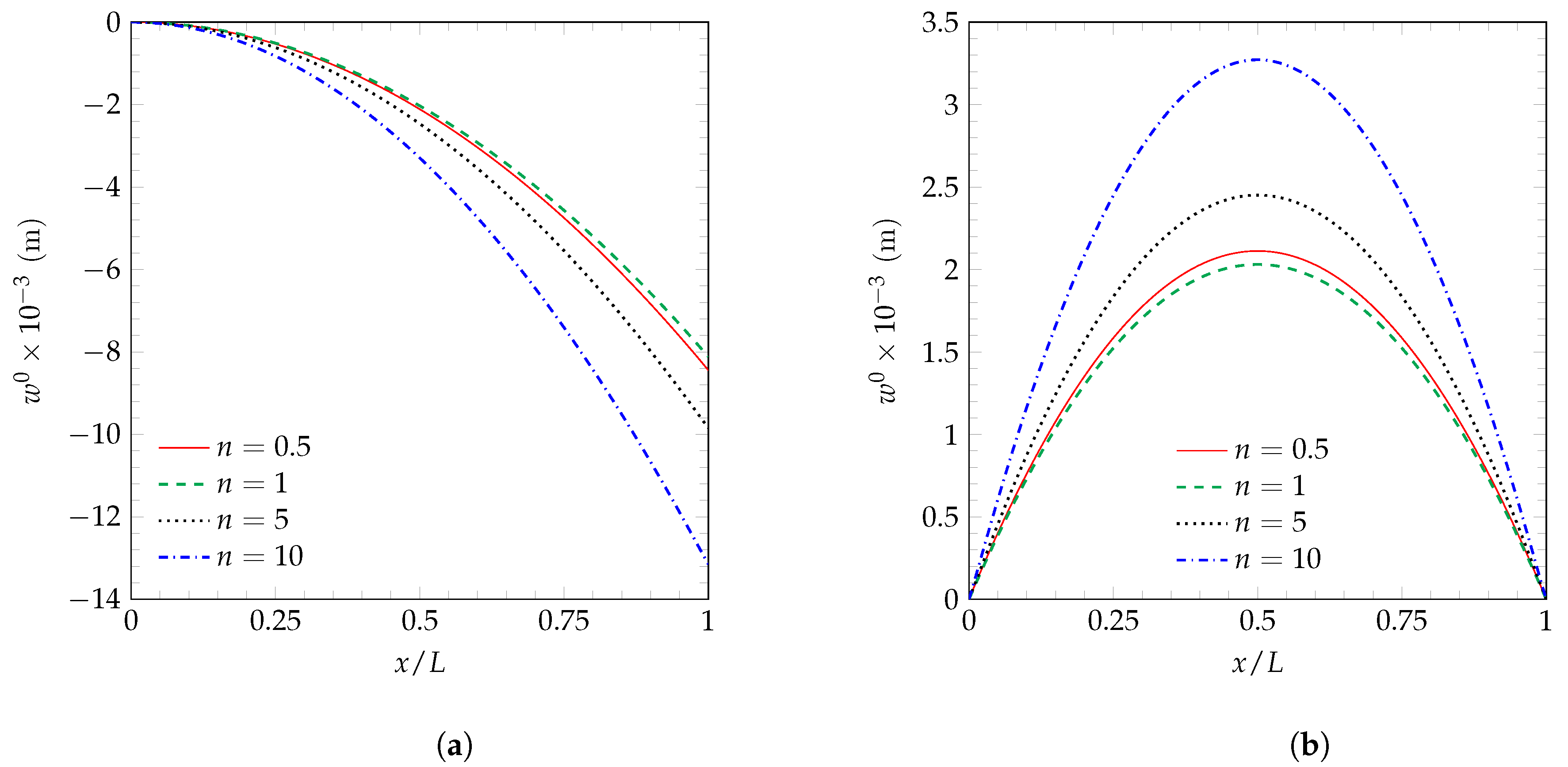
To complement the above numerical results, Figure 2 shows the transverse deflection for various power law exponents of FG beams subjected to thermal and mechanical loads. Figure 2a,b shows the transverse deflection of C-F and S-R FG beams, respectively. For both boundary conditions, the minimum transverse deflection is obtained when $n=1$.

4.5. Thermal–Structural Analysis of FG Beams, for $n=1$

In this section, the thermo-mechanical response of the FG beam with a power law exponent $n=1$ is studied for the C-F and an S-R boundary conditions. For this analysis, a distributed load $q_0=-{10}^4$ N/m was applied to the FG beam, and the top surface temperature was considered to vary, while the other temperatures remained fixed; that is, the temperature of reference and bottom surface temperature were considered to be constant with the following values: $T_{ref}=0$ °C and $T_{bot}=20$ °C. The latter consideration allowed us to obtain the behavior of the FG beam as it is exposed to various temperature differences between its top and bottom surfaces, such that $\Delta T=T_{top}-T_{ref}$. Moreover, several length-to-thickness ratios were studied.

The maximum axial displacements and transverse deflections for the C-F FG beam are presented in

Table 12. Maximum displacements of a C-F FG beam $(n=1)$ subjected to various $\Delta T$ and a distributed load $q_0=-{10}^4$ N/m ($T_{bot}=20$ °C and $T_{ref}=0 °\mathrm{C}$).

		$\mathbf{\Delta }\mathit{T}=100 °\mathbf{C}$		$\mathbf{\Delta }\mathit{T}=200 °\mathbf{C}$		$\mathbf{\Delta }\mathit{T}=300 °\mathbf{C}$		$\mathbf{\Delta }\mathit{T}=400 °\mathbf{C}$
$\mathit{L}/\mathit{h}$	Model	${\mathit{u}}^0\times {10}^{-3}$	${\mathit{w}}^0\times {10}^{-3}$	${\mathit{u}}^0\times {10}^{-3}$	${\mathit{w}}^0\times {10}^{-3}$	${\mathit{u}}^0\times {10}^{-3}$	${\mathit{w}}^0\times {10}^{-3}$	${\mathit{u}}^0\times {10}^{-3}$	${\mathit{w}}^0\times {10}^{-3}$
3	Present	1.8938	$-1.5267$	2.8760	$-4.4503$	3.8582	$-7.3739$	4.8403	$-10.2976$
	Plane	1.9195	$-1.5620$	2.9150	$-4.5445$	3.9105	$-7.5270$	4.9060	$-10.5100$
5	Present	3.1554	$-4.2698$	4.7924	$-12.3883$	6.4293	$-20.5069$	8.0662	$-28.6255$
	Plane	3.1814	$-4.2973$	4.8320	$-12.4920$	6.4826	$-20.6870$	8.1332	$-28.8810$
10	Present	6.3018	$-17.6686$	9.5756	$-50.1384$	12.8495	$-82.6082$	16.1234	$-115.0780$
	Plane	6.3288	$-17.7010$	9.6176	$-50.3030$	12.9060	$-82.9060$	16.1950	$-115.5100$
20	Present	12.5308	$-80.1733$	19.0785	$-210.0480$	25.6263	$-339.9227$	32.1740	$-469.7974$
	Plane	12.5620	$-80.1610$	19.1300	$-210.1200$	25.6980	$-340.0800$	32.2660	$-470.0300$

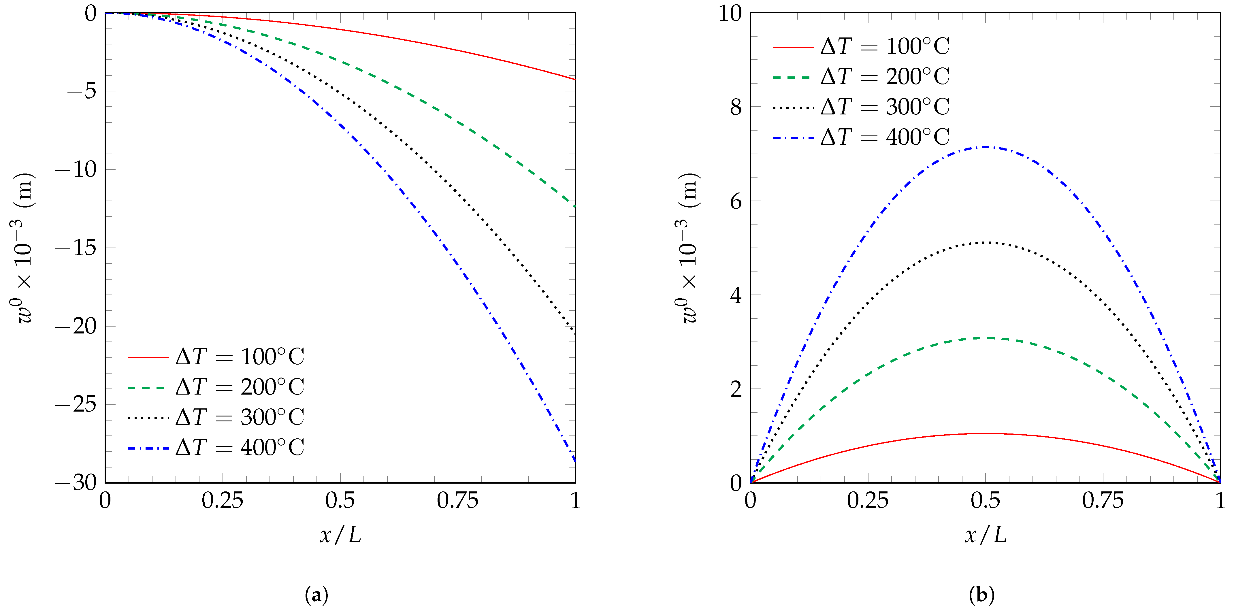
; also, numerical results obtained using the plane model are included for comparison purposes. The influence of increasing the top surface temperature can be noted as an increment in both displacements, and the maximum displacements are obtained when $\Delta T=400$ °C. In addition, a plot of the transverse deflection along the x axis of the FG beam is shown in Figure 3a, where greater deflections are observed as the temperature of the top surface increases.

The comparisons of the results presented in Table 12 give the following ranges for the relative errors (${\epsilon }_r$):

• $L/t=3$: $1.34\le {\epsilon }_r\le 2.26\%$.
• $L/t=5$: $0.64\le {\epsilon }_r\le 0.88\%$.
• $L/t=10$: $0.18\le {\epsilon }_r\le 0.44\%$.
• $L/t=20$: $0.02\le {\epsilon }_r\le 0.29\%$.

As noted before, higher values of relative errors are obtained for the C-F FG beam of ratio $L/t=3$. For moderately short to long beams, the values are below $0.9\%$. Therefore, the present model shows good behavior for the thermo-mechanical response of FG beams at different temperatures.

Now, regarding the S-R FG beam, the axial displacements and transverse deflections are presented in

Table 13. Maximum displacements of an S-R FG beam $(n=1)$ subjected to various $\Delta T$ and a distributed load $q_0=-{10}^4$ N/m ($T_{bot}=20$ °C and $T_{ref}=0 °\mathrm{C}$).

		$\mathbf{\Delta }\mathit{T}=100 °\mathbf{C}$		$\mathbf{\Delta }\mathit{T}=200 °\mathbf{C}$		$\mathbf{\Delta }\mathit{T}=300 °\mathbf{C}$		$\mathbf{\Delta }\mathit{T}=400 °\mathbf{C}$
$\mathit{L}/\mathit{h}$	Model	${\mathit{u}}^0\times {10}^{-3}$	${\mathit{w}}^0\times {10}^{-3}$	${\mathit{u}}^0\times {10}^{-3}$	${\mathit{w}}^0\times {10}^{-3}$	${\mathit{u}}^0\times {10}^{-3}$	${\mathit{w}}^0\times {10}^{-3}$	${\mathit{u}}^0\times {10}^{-3}$	${\mathit{w}}^0\times {10}^{-3}$
3	Present	1.8943	$0.3802$	2.8765	$1.1122$	3.8587	$1.8443$	4.8408	$2.5763$
	Plane	1.8927	$0.3807$	2.8732	$1.1131$	3.8538	$1.8455$	4.8343	$2.5779$
5	Present	3.1577	$1.0502$	4.7946	$3.0809$	6.4316	$5.1117$	8.0685	$7.1425$
	Plane	3.1563	$1.0540$	4.7919	$3.0882$	6.4276	$5.1224$	8.0632	$7.1565$
10	Present	6.3199	$4.1343$	9.5938	$12.2529$	12.8677	$20.3715$	16.1416	$28.4900$
	Plane	6.3194	$4.1525$	9.5931	$12.2840$	12.8670	$20.4170$	16.1400	$28.5490$
20	Present	12.6762	$15.5429$	19.2240	$48.0127$	25.7718	$80.4825$	32.3195	$112.9523$
	Plane	12.6790	$15.5870$	19.2310	$48.0440$	25.7840	$80.5010$	32.3370	$112.9600$

. In this case, the similarities with the axial displacements of C-F FG beam are only observed in short beams; notable differences are observed as the length-to-thickness ratio increases. The transverse deflection of the S-R FG beam is shown in Figure 3b, where again greater deflections are observed as the temperature of the top surface increases.

The ranges of relative errors for the results presented in Table 13 are

• $L/t=3$: $0.06\le {\epsilon }_r\le 0.13\%$.
• $L/t=5$: $0.04\le {\epsilon }_r\le 0.36\%$.
• $L/t=10$: $0.01\le {\epsilon }_r\le 0.44\%$.
• $L/t=20$: $0.01\le {\epsilon }_r\le 0.28\%$.

From Table 12 and Table 13, it can be observed that the displacements have similar behavior as presented in the static analyses of FG beams; that is, for a larger length-to-thickness ratio, higher displacements and deflections are presented. Furthermore, higher displacements and deflections are obtained as the temperature of the top surface increases, which is expected since the thermal effects also depend on $\Delta T$.

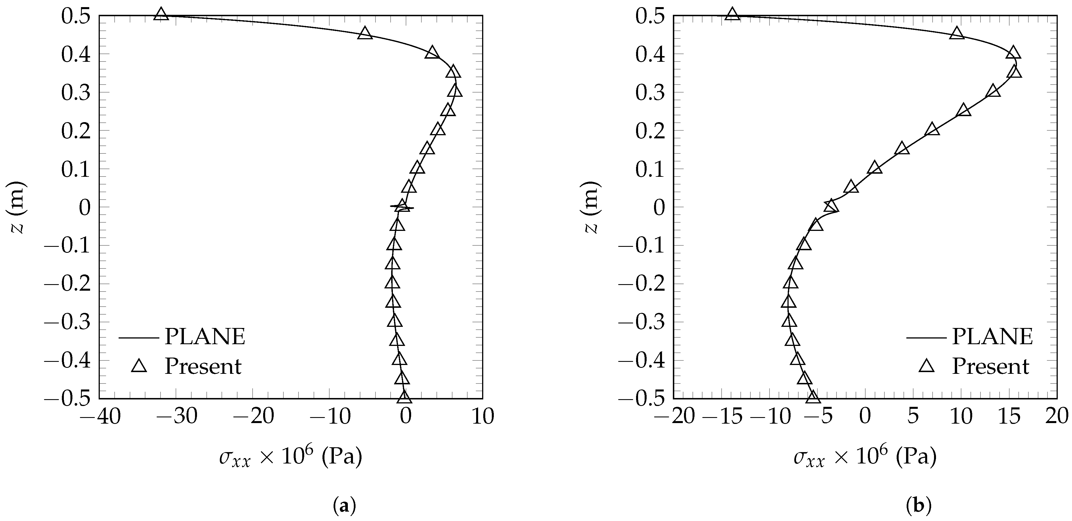
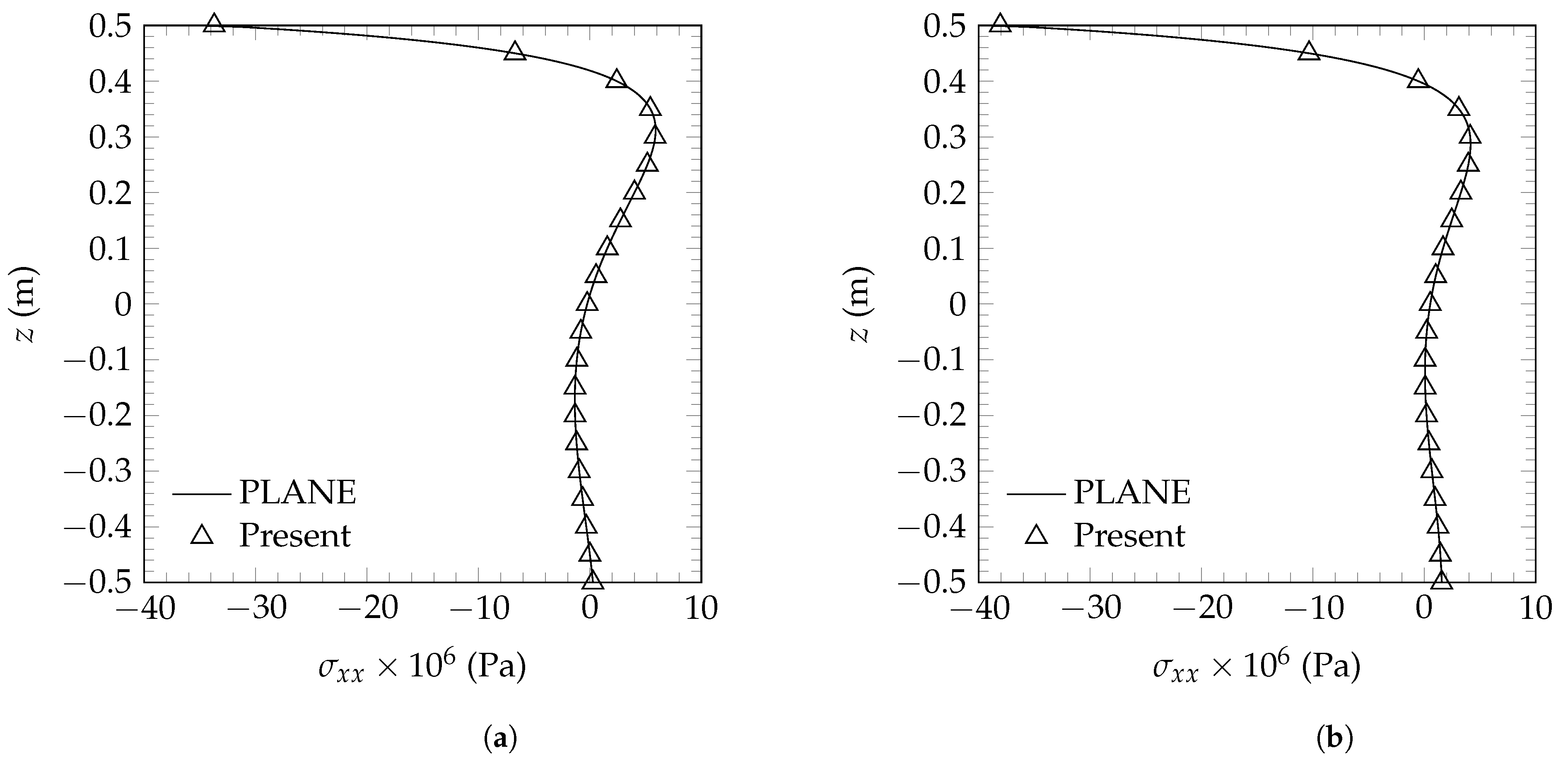
In addition to the displacements presented in Table 12, the normal stresses through the thickness of a C-F FG beam with $n=1$ at the clamped end are shown in Figure 4 for the ratios $L/t=5$ and $L/t=20$. Additionally, the normal stress obtained by means of the plane model is plotted to compare with the present model’s results; from this comparison, a similar behavior of both models is observed. The normal stress is highly influenced by the length-to-thickness ratio since significant variations are observed in the FG beam with $L/t=20$. It should be recalled that, in accordance with the temperature distribution and the temperatures considered, higher contributions due to thermal effects are observed at the top surface, where the difference $T\left(z\right)-T_{ref}$ reaches its maximum value.

In addition to the results presented in Table 13 for an S-R FG beam with $n=1$, the variation of the normal stress through the thickness at the mid-span is shown in Figure 5 for the ratios $L/t=5$ and $L/t=20$. In the case of S-R conditions, contrary to the C-F condition, a significant influence of the length-to-thickness ratio is not observed on the normal stress.

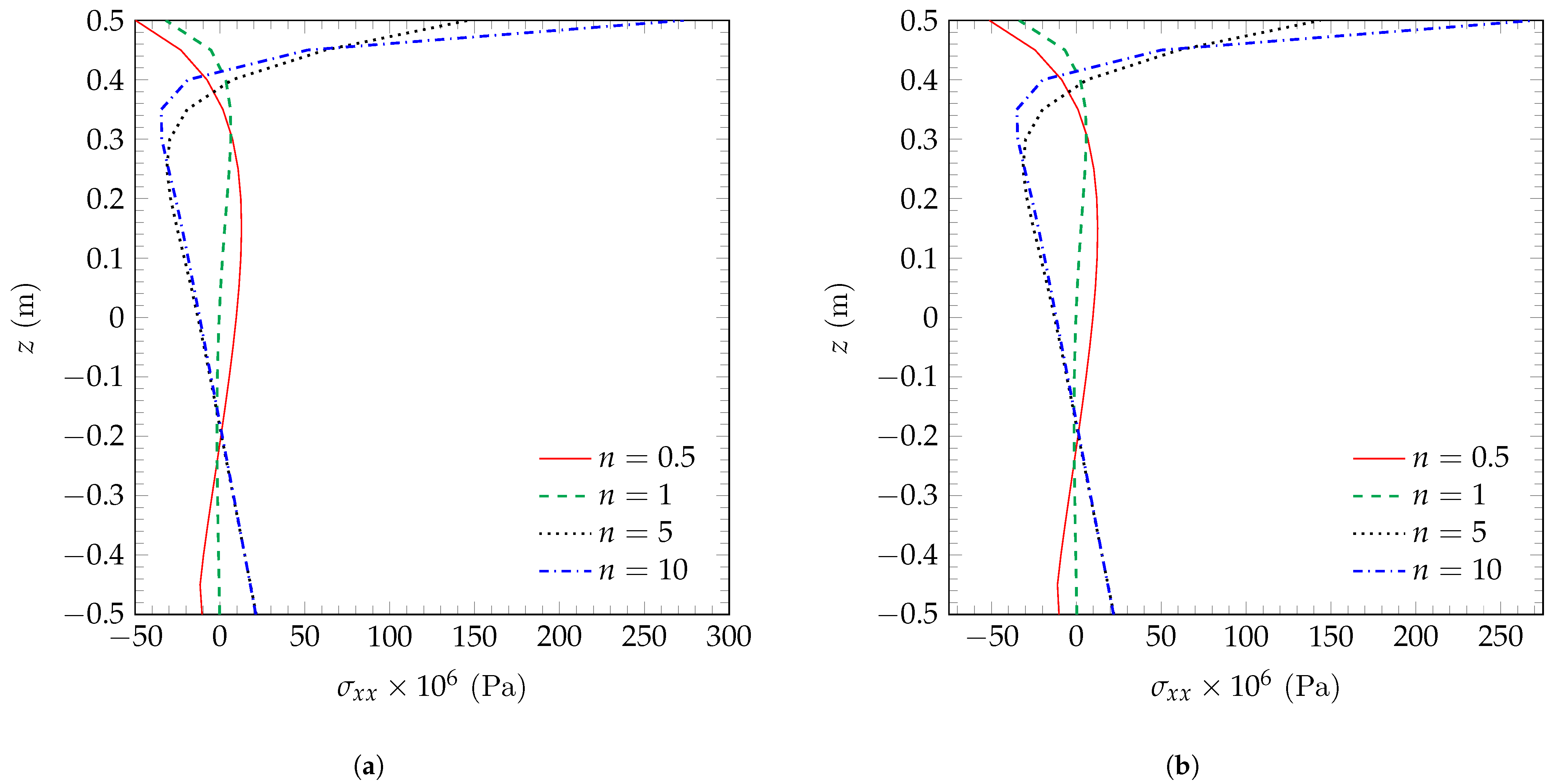
For completeness, the behavior of the normal stress when $\Delta T=100$ °C for different values of the power law exponent n and a length to thickness ratio $L/t=5$ is presented in Figure 6. It can be observed that, the behavior is similar for the C-F and S-R boundary conditions, with the maximum tensile stress being achieved for higher values of n (for the results presented here, it occurs when $n=10$).

5. Conclusions

In this paper, a finite element model based on TSDT to obtain the thermo-mechanical responses of FG beams subjected to distributed loads and thermal loads was presented. Moreover, the verification of the model’s behavior was made in the following order: the mechanical response of FG beams, the thermo-mechanical response of isotropic beams, and, finally, the thermo-mechanical response of FG beams. The latter verification is made by a comparison with the results obtained using plane elements. Slight variations are expected in the comparisons since the formulation of the present model is distinct from the formulations used in the literature and simulations. In general, the following conclusions can be drawn:

• The present finite element model incorporated the rule of mixtures to evaluate the effective mechanical and thermal properties of the FG constituents, where the volume distribution of the ceramic was considered by means of the power law.
• The behavior of the present finite element model was checked by a comparison with the literature and simulations in a finite element commercial code, with the findings showing that the aforementioned results are close to the present ones and behave in a similar manner. Maximum axial displacements and transverse deflections are now available for a comparison with studies that have dealt with the thermal–structural problem presented here.
• In the thermal–structural analysis of FG beams subject to the boundary conditions considered in this article, the higher relative errors were obtained when short beams (e.g., $L/h=3$) were modeled.
• In addition, we found that normal stresses predicted by the present finite element model were in good agreement with those obtained using plane elements.

References

1. Chakraborty, A.; Gopalakrishnan, S.; Reddy, J. A new beam finite element for the analysis of functionally graded materials. Int. J. Mech. Sci. 2003, 45, 519–539. [Google Scholar] [CrossRef]
2. Elishakoff, I.E.; Pentaras, D.; Gentilini, C. Mechanics of Functionally Graded Material Structures; World Scientific: Singapore, 2015. [Google Scholar]
3. Ebrahimi, F.; Jafari, A. A four-variable refined shear-deformation beam theory for thermo-mechanical vibration analysis of temperature-dependent FGM beams with porosities. Mech. Adv. Mater. Struct. 2018, 25, 212–224. [Google Scholar] [CrossRef]
4. Xia, Y.M.; Li, S.R.; Wan, Z.Q. Bending solutions of FGM Reddy–Bickford beams in terms of those of the homogenous Euler–Bernoulli beams. Acta Mech. Solida Sin. 2019, 32, 499–516. [Google Scholar] [CrossRef]
5. Mahamood, R.; Jen, T.; Akinlabi, S.; Hassan, S.; Shatalov, M.; Murashkin, E.; Akinlabi, E.T. Functionally Graded Materials: An Introduction. In Functionally Graded Materials (FGMs); CRC Press: Boca Raton, FL, USA, 2021; pp. 1–12. [Google Scholar]
6. Giunta, G.; Crisafulli, D.; Belouettar, S.; Carrera, E. A thermo-mechanical analysis of functionally graded beams via hierarchical modelling. Compos. Struct. 2013, 95, 676–690. [Google Scholar] [CrossRef]
7. De Pietro, G.; Hui, Y.; Giunta, G.; Belouettar, S.; Carrera, E.; Hu, H. Hierarchical one-dimensional finite elements for the thermal stress analysis of three-dimensional functionally graded beams. Compos. Struct. 2016, 153, 514–528. [Google Scholar] [CrossRef] [Green Version]
8. Malik, P.; Kadoli, R. Thermo-elastic response of SUS316-Al2O3 functionally graded beams under various heat loads. Int. J. Mech. Sci. 2017, 128–129, 206–223. [Google Scholar] [CrossRef]
9. El-Megharbel, A. A theoretical analysis of functionally graded beam under thermal loading. World J. Eng. Technol. 2016, 4, 437–449. [Google Scholar] [CrossRef]
10. Li, X.F. A unified approach for analyzing static and dynamic behaviors of functionally graded Timoshenko and Euler–Bernoulli beams. J. Sound Vib. 2008, 318, 1210–1229. [Google Scholar] [CrossRef]
11. Alshorbagy, A.E.; Eltaher, M.; Mahmoud, F. Free vibration characteristics of a functionally graded beam by finite element method. Appl. Math. Model. 2011, 35, 412–425. [Google Scholar] [CrossRef]
12. Moheimani, R.; Ahmadian, M.T. On free vibration of functionally graded Euler-Bernoulli beam models based on the non-local theory. In Vibration, Acoustics and Wave Propagation, Proceedings of the ASME International Mechanical Engineering Congress and Exposition, Houston, TX, USA, 9–15 November 2012; ASME: New York, NY, USA, 2012; Volume 12, pp. 169–173. [Google Scholar]
13. Nguyen, T.K.; Vo, T.P.; Thai, H.T. Static and free vibration of axially loaded functionally graded beams based on the first-order shear deformation theory. Compos. Part B Eng. 2013, 55, 147–157. [Google Scholar] [CrossRef] [Green Version]
14. Katili, I.; Syahril, T.; Katili, A.M. Static and free vibration analysis of FGM beam based on unified and integrated of Timoshenko’s theory. Compos. Struct. 2020, 242, 112130. [Google Scholar]
15. Kadoli, R.; Akhtar, K.; Ganesan, N. Static analysis of functionally graded beams using higher order shear deformation theory. Appl. Math. Model. 2008, 32, 2509–2525. [Google Scholar] [CrossRef]
16. Aydogdu, M.; Taskin, V. Free vibration analysis of functionally graded beams with simply supported edges. Mater. Des. 2007, 28, 1651–1656. [Google Scholar] [CrossRef]
17. Mahi, A.; Adda Bedia, E.; Tounsi, A.; Mechab, I. An analytical method for temperature-dependent free vibration analysis of functionally graded beams with general boundary conditions. Compos. Struct. 2010, 92, 1877–1887. [Google Scholar] [CrossRef]
18. Thai, H.T.; Vo, T.P. Bending and free vibration of functionally graded beams using various higher-order shear deformation beam theories. Int. J. Mech. Sci. 2012, 62, 57–66. [Google Scholar] [CrossRef] [Green Version]
19. Vo, T.P.; Thai, H.T.; Nguyen, T.K.; Inam, F. Static and vibration analysis of functionally graded beams using refined shear deformation theory. Meccanica 2014, 49, 155–168. [Google Scholar]
20. Şimşek, M.; Reddy, J.N. Bending and vibration of functionally graded microbeams using a new higher order beam theory and the modified couple stress theory. Int. J. Eng. Sci. 2013, 64, 37–53. [Google Scholar]
21. Gao, X.L.; Zhang, G.Y. A microstructure- and surface energy-dependent third-order shear deformation beam model. Z. Angew. Math. Phys. 2015, 66, 1871–1894. [Google Scholar]
22. Chakraborty, A.; Gopalakrishnan, S. A spectrally formulated finite element for wave propagation analysis in functionally graded beams. Int. J. Solids Struct. 2003, 40, 2421–2448. [Google Scholar] [CrossRef]
23. Daneshmehr, A.R.; Mohammad Abadi, M.; Rajabpoor, A. Thermal effect on static bending, vibration and buckling of Reddy beam based on modified couple stress theory. Appl. Mech. Mater. 2013, 332, 331–338. [Google Scholar] [CrossRef]
24. Lim, T.K.; Kim, J.H. Thermo-elastic effects on shear correction factors for functionally graded beam. Compos. Part B Eng. 2017, 123, 262–270. [Google Scholar] [CrossRef]
25. Praveen, G.N.; Reddy, J.N. Nonlinear transient thermoelastic analysis of functionally graded ceramic-metal plates. Int. J. Solids Struct. 1998, 35, 4457–4476. [Google Scholar] [CrossRef]
26. Javaheri, R.; Eslami, M.R. Thermal buckling of functionally graded plates. AIAA J. 2002, 40, 162–169. [Google Scholar] [CrossRef]
27. Reddy, J.N. On locking-free shear deformable beam finite elements. Comput. Methods Appl. Mech. Eng. 1997, 149, 113–132. [Google Scholar] [CrossRef]
28. Reddy, J.N. Energy Principles and Variational Methods in Applied Mechanics; John Wiley & Sons: Hoboken, NJ, USA, 2002. [Google Scholar]
29. Şimşek, M. Static analysis of a functionally graded beam under a uniformly distributed load by Ritz method. Int. J. Eng. Appl. Sci. 2009, 1, 1–11. [Google Scholar]
30. Hetnarski, R.B.; Eslami, M.R. Solid Mechanics and Its Applications. In Thermal Stresses—Advanced Theory and Applications; Springer: Dordrecht, The Netherlands, 2009; Volume 158. [Google Scholar]
Figure 1. FG beam subjected to a distributed load with different temperatures of the top and bottom surfaces.
Mca 28 00084 g001
Figure 2. Transverse deflection of various FG beams subjected to thermal and distributed loads where q 0 = 100 N/m ( T t o p = 400 °C, T b o t = 300 °C, and T r e f = 300 °C) under (a) C-F and (b) S-R boundary conditions.
Mca 28 00084 g002
Figure 3. Transverse deflection of FG beams ( n = 1 ) subjected to various Δ T and a distributed load q 0 = 10 4 N/m ( T b o t = 20 °C and T r e f = 0   ° C ) under (a) C-F and (b) S-R boundary conditions.
Mca 28 00084 g003
Figure 4. Variation of the normal stress σ x x of a C-F FG beam subjected to a mechanical and thermal load for n = 1 and (a) L / h = 5 ; (b) L / h = 20 ( q 0 = 10 4 N/m, T b o t = 20 °C, and T r e f = 0   ° C ).
Mca 28 00084 g004
Figure 5. Variation of the normal stress σ x x of an S-R FG beam subjected to a mechanical and thermal load for n = 1 and (a) L / h = 5 ; (b) L / h = 20 ( q 0 = 10 4 N/m, T b o t = 20 °C, and T r e f = 0   ° C ).
Mca 28 00084 g005
Figure 6. Normal stress ( σ x x ) of various FG beams subjected to thermal and distributed loads where q 0 = 10 4 N/m ( T t o p = 120 °C, T b o t = 20 °C, and T r e f = 0 °C) under (a) C-F and (b) S-R boundary conditions.
Mca 28 00084 g006