
Accuracy Examination of the Fourier Series Approximation for Almost Limiting Gravity Waves on Deep Water


1
Department of Marine Environment and Engineering, National Sun Yat-Sen University, Kaohsiung 804, Taiwan
2
Department of Civil Engineering, National Yangming Chiaotung University, Hsinchu 300, Taiwan
*
Author to whom correspondence should be addressed.
Math. Comput. Appl. 2024, 29(1), 5; https://doi.org/10.3390/mca29010005
Submission received: 21 December 2023
/
Revised: 1 January 2024
/
Accepted: 4 January 2024
/
Published: 11 January 2024
(This article belongs to the Collection Feature Papers in Mathematical and Computational Applications 2024)
Abstract
:A permanent gravity wave propagating on deep water is a classic mathematical problem. However, the Fourier series approximation (FSA) based on the physical plane was examined to be valid for almost waves at all depths. The accuracy of the FSA for almost-limiting gravity waves remains unevaluated, which is the purpose of this study. We calculate some physical properties of almost-limiting waves on deep water using the FSA and compare them with other studies on the complex plane. The comparison results show that the closer the wave is, the greater the difference. We find that the main reason for this difference is that the wave profile in the FSA retains an original implicit form and is not represented by Fourier series. Therefore, the kinematic and dynamic conditions of the free surface around the wave crest cannot be satisfied at the same time.
1. Introduction
The weak nonlinearity of a permanent two-dimensional finite-amplitude gravity wave was first investigated by Stokes [1] using a perturbation approach. Among the analytical approaches for this problem of finite-amplitude Stokes waves, perturbation methods have been used most frequently, such as Skjelbreia and Hendrickson [2], Isobe et al. [3], and Fenton [4]. However, Stokes [5] first proved that the limiting Stokes wave has a sharp angle on the crest. Such a corner forms a slope jump on both sides of the crest to indicate that the summit has one singularity of order 2/3. Grant [6] pointed out that for any lesser amplitude, it has singularities of the order 1/2 only. The only way to take a continuous approach to the greatest amplitude possible is to have several coalescing singularities. The Stokes conjecture was later proved [7,8,9,10].
Beyond the limiting wave, a permanent gravity wave propagating on deep water is a classic physical and mathematical problem of amplitudes varying from small to steep amplitudes. With the help of excellent algorithms of numerical computation, the high nonlinearity of almost-limiting gravity waves, even up to the limiting case, has been widely studied by many researchers [11,12,13,14,15,16,17,18,19,20,21,22], in which the FSA developed by Rienecker and Fenton [22] serves as the methodological basis for this study. Maklakov [23] proposed a method to calculate two full periods of the oscillations of the wave properties for all height-to-length ratios of the waves. The end of the second period corresponds to the wave steepness that achieves 99.99997% of the limiting wave of a finite depth. Clamond and Dutykh [24] proposed an accurate and fast computation of steady two-dimensional surface gravity waves at an arbitrary depth.
Chandler and Graham [25] pointed out that the singularity of the limiting wave explains a slow convergence of the Stokes expansion or causes a Benjamin–Feir instability. The location of the main singularity was identified using techniques in series acceleration [13,15,26,27,28,29]. Graves-Morris [30] explained that branch points in an analytically continued function will typically manifest as sequences of poles in a Padé approximant. The presence of a branch-point singularity was constructed by some researchers [31,32,33,34,35].
According to previous works, a singularity existing on the crest of the limiting wave causes the physical region to become non-analytic. Steep periodic gravity waves on water of a finite type have been the subject of intensive investigation. Most numerical methods encounter difficulties with waves close to the limiting configuration. Many physical phenomena and mathematical problems related to surface gravity water waves remain unknown, not well understood, or unsolved, even in the “simple” case of travelling waves of a permanent form in two-dimensional irrotational motion [36,37].
In addition to the limiting wave, this paper investigates a two-dimensional periodic gravity wave on deep water using the FSA. The FSA is a common numerical method to reduce free surface conditions to a set of nonlinear equations by simultaneously satisfying a number of points on the surface, which is called the collation method. Rienecker and Fenton [22] compared the results of wave speed squared by the Fourier method with different N values with those of Cokelet [16] and Vanden-Broeck and Schwartz [38] for a moderately long wave and examined the accuracy of the Fourier method with N = 16, finding that the approximation did not converge to a solution for the limiting wave; however, it was still accurate up to 97% as high as the largest. An efficient and fast computation was developed for pure solitary waves by Clamond and Dutykh [39] and Dutykh and Clamond [40] or for generalized solitary gravity-capillary water waves by Clamond et al. [41] and Dutykh et al. [42]. Zhong and Liao [43] used the homotopy analysis method (HAM) to perform a convergent computation for the limiting Stokes waves in an arbitrary water depth and solitary waves in extremely shallow water.
Rienecker and Fenton [22] applied the FSA to compute physical quantities varying with position and time, which are physical quantities characteristic of the wave train. Furthermore, through comparisons of two experiments which measure fluid velocities under the crest in a wave tank, a better agreement between the FSA with N = 8 and these experiments than other analytical theories indicates the physical validity of the FSA, and the results for N = 16 and 32 were indistinguishable from the result for N = 8. Rienecker and Fenton [22] described the FSA algorithm for wave shoaling and made comparisons with the experiments of Hansen and Svendsen [44]. The results showed quite a good agreement.
The motion of a paddle with regular oscillation in a two-dimensional flume can produce progressive waves and a series of standing (evanescent) waves, of which the amplitudes decay exponentially with distance from the wavemaker (Dean and Dalrymple [45]). However, Vivanco et al. [46] proposed the pedal-wavemaking method to generate a regular surface wave excluding evanescent waves. The proper synchronization of the orbital motion on the bottom can emulate deep-water behavior according to the linear Airy theory. When the wavemaker moves with large displacements, there are significant nonlinear effects between these waves and the paddle motion that occur to form the waves of different sizes and shapes at different locations away from the wavemaker. The sharpness of the crest for the very highest and longest waves due to a high non-linearity cannot be solved. Therefore, experiments on the kinematic characteristics of large waves on a flat bottom are still unavailable, regardless of the results of almost-limiting waves.
Rienecker and Fenton [22] concluded that the FSA is essentially a numerical technique for the approximation of continuous periodic functions and is valid for almost waves at all depths. After using Fourier series to represent the surface wave profile, Newton’s iteration method associated with relaxation technology was used to solve the unknowns of the simultaneous nonlinear equations by Zhao et al. [47]. The application of the FSA to the shoaling of nonlinear waves over a gently sloping bottom was studied by Chang [48] and Eldrup and Andersen [49]. Chang et al. [50] used the FSA to calculate the particle trajectory of nonlinear gravity waves on deep water. Nonlinear effects resulting from using the FSA produce a larger motion than the fifth-order approximation [51]. The calculated mass transport of the particle on the water surface is quite similar to that of Longuet-Higgins [52].
Although the FSA has proven to have a considerable accuracy when used on small to large waves at all water depths, the FSA has not yet been evaluated for use on almost-limiting Stokes waves. The main purpose of this paper is to compare the differences between the physical properties of almost-limiting waves calculated by the FSA and some previous methods and to analyze the errors and limitations of the use of the FSA. In the Introduction section, we mainly review the literature on the calculation of Stokes waves and the characteristics of the limiting waves. The formulation of the problem in a physical plane and the FSA algorithm are introduced in Section 2. In the third section, some physical properties are calculated using the FSA for all possible waves. The results are compared with those of Cokelet [14], Williams [18], and Longuet-Higgins and Tanaka [53], based on the same corresponding parameters. The celerity of the almost-limiting wave is compared with that obtained using the empirical formula of Lushnikov et al. [35]. The angled crests and inner profiles obtained using KFSBC and DFSBC for four almost-limiting waves show differences, showing the poor accuracy of the FSA and the limit of governing equations in a physical plane. The height of the singularity on the crest of the limiting waves is computed using the FSA. The last section leads to a remarkable conclusion.
2. Methods
2.1. Governing Equations
Consider two-dimensional and periodic, pure gravity waves of a permanent type propagating with a constant speed, c, from right to left on a deep water. Assume that the fluid is inviscid and incompressible and that the motion is irrotational. For the problem, a frame of reference that moves with the wave celerity is easier to describe the motion with than a fixed frame. Choose rectangular Cartesian coordinates (x, y) such that the x axis is horizontal, the y axis is directed vertically upward, and propagation passes through the wave crest. The origin lies at the mean water level.
A stream function, φ(x, y), satisfies Laplace’s equation and indicates the velocity, (u, v), by the definition of u = φy and v = −φx, in which the subscripts denote the partial derivatives.
where η(x) is the free surface. The boundary conditions imposed on the flow are that the free surface is a streamline, and the pressure along the free surface is assumed to be equal and to satisfy the Bernoulli equation.
where Q is the value of the stream function on the surface, B is the Bernoulli constant, and g is the gravitational acceleration. Equations (2) and (3) are the kinematic and dynamical boundary conditions on the free surface. The fluid at an infinite depth remains still under a propagating wave so that the horizontal component of the fluid velocity at an infinite depth is −c in the opposite direction relative to the moving reference. The bottom boundary condition yields
Assuming that the wave is periodic along the x-axis and symmetric about the crest, Equation (1) admits a general solution in the Fourier series.
where Bn (n = 0, 1, …) are unknown coefficients for a specified wave, k = 2π/L is the wave number, and L is the wave length. Equation (5) already satisfies Equation (4) but does not satisfy Equations (2) and (3) yet. So far, Equation (5) is not an exact particular solution for a specified wave.
Since the free surface η(x) is unknown and the equation of the dynamic boundary condition on the free surface is non-linear, all coefficients of the infinite Fourier series are difficult to obtain using analytical methods in mathematics. Numerical results with high-order approximations have been taken as “exact solutions” of this problem.
2.2. FSA’s Algorithm
The FSA, first introduced by Rienecker and Fenton [22], is applied to obtain the solution of the almost-limiting gravity waves on deep water. The FSA can give a direct solution in that the values of the stream function, and the surface elevations are obtained as a function of position. Moreover, it does not depend on the wave being small and is valid for all depths. Rienecker and Fenton [22] showed that the FSA gave highly accurate results up to a point equal to about 99% of the maximum wave height but did not converge to a solution for almost-limiting waves. In this paper, a breaking condition is employed to overcome the difficulty in numerical convergence.
To facilitate the numerical computation in Equation (5), the number of terms is limited to N. A set of N + 1 equispaced points on the free surface, from the wave crest to the trough, is chosen to satisfy Equations (2) and (3). Hence, the governing equations are given below.
where ηj = η(xj) at kxj = jπ/N. The x and y components of a particle velocity at ηj, uj, and vj are given by
Equations (6) and (7) represent a system of 2N + 2 nonlinear equations with 2N + 4 unknowns, namely, Bn (n = 1, …, N), ηj (j = 0, 1, …, N), c, Q, and B. Thus, two additional equations are required to solve the unknowns. Given that the mean water level is equal to zero, as required by mass conservation, the equation can be written using Simpson’s one-third rule for the numerical integration of a periodic function.
Rienecker and Fenton [22] introduced an additional equation for nonbreaking waves of a specified wave height.
However, in a limiting wave, the wave height is unknown, so it is necessary to introduce another supplementary equation. If wave breaking is to occur, the particle speed at the very crest must be at least equal to the phase speed. Therefore, the Rankine breaking condition is defined by the fact that at the very crest the water moves at the same speed as the wave profile. In the steady state, the fluid velocity at the summit is equal to zero, uc(x = 0) = 0, when the wave breaks.
Schwartz [12] used a perturbation approach and gained the perturbation expansion at the 117th order on deep water and at the 48th order in general water depths, respectively. Using the Padé approximants and the Shanks transformation, Schwartz [12] successfully obtained the wave speed as a function of the wave height for waves from the lowest to near the highest for a variety of water depths. However, his method converges only well for wave heights less than 97% of the maximum.
Longuet-Higgins and Fenton [54] considered an expansion parameter defined as 1 − (uc/c0)2
where c0 is the phase speed of waves with an infinitesimal amplitude. This parameter has the advantage that its range, 0 ≤ ≤ 1, is known beforehand. Thus, = 0 corresponds to the wave with an infinitesimal amplitude, while = 1 corresponds to the limiting wave with a stagnation point at the crest due to uc = 0. By this parameter, Longuet-Higgins and Fenton [54] found that the series under the use of Padé approximants converge well.
In addition, Longuet-Higgins [55] used another expansion parameter.
where ut denotes the speed of the fluid in the trough. For an infinitesimal wave, uc = ut = c = c0 so that ω = 0. For the limiting wave, ω = 1. This parameter has a similar range, 0 ≤ ω ≤ 1. Longuet-Higgins [55] obtained a series in ω, and there was a rapid convergence.
Cokelet [14] chose a new expansion parameter defined as
Cokelet [14] pointed out that this parameter has four attributes, that is, (1) its range 0 ≤ ε ≤ 1 is known; (2) most physical properties of the flow are expressed in series in even powers of ε; (3) the perturbation expansion can be carried out initially in terms of ε without having to resort to series reversion; and (4) the resulting series in ε can be summed with Padé approximants giving rapid convergence.
Tanaka [56] distinguished waves of a given amplitude from the infinitesimal wave to the limiting wave by a parameter defined as
The parameter is suitable as the amplitude parameter because its range is known a priori to be 0 ≤ ≤ 1.
Equations (6), (7), (10) and (11), and one of Equations (12)–(15), form a closed system of 2N + 5 nonlinear equations. The FSA is a kind of collation method. The limiting Stokes wave has a singularity in the form of a sharp angle of 2π/3 radians on the crest [4]. Grant [6] found that the corner singularity might not be a simple algebraic branch point because other types of singularity expressed in a power of the transcendental number might exist. The existence of a limiting Stokes wave with the inclination of the slope at the crest was proved by Grant [6]. The main singularity of the limiting wave arises with great difficulty in the solution because of the branch points and Riemann surfaces. However, some rigorous results on asymptotics near the crest of the limiting wave have been investigated [8,31,32,48,49,50,51,52].
The set of 2N + 5 nonlinear equations excluding the singularity of the limiting wave is analytical and is suitable for waves from small-amplitude waves to the almost-limiting waves. Therefore, the limiting wave is excluded in the paper. The solution of the 2N + 5 unknown variables was solved and programmed using Newton’s method which iterates, with quadratic convergence to a solution from an initial approximation. All the quantities in these equations are nondimensionalized by virtue of g and k. The nonlinear 2N + 5 equations can be written in a general form, fi (zj), in terms of the z vector of arguments, zj, which are Bn (n = 1, 2, …, N), ηj (j = 0, 1, …, N), c, Q, B, and H.
When all functions and variables in the k-th iteration using Newton’s method with 2N + 5 variables are set in the column vectors f and zk, the desired results zk+1 after the next iteration can be obtained from algebraic linear equations to make the absolute values of f(zk+1) less than the specified tolerance, 10−10, in this study. The computation starts with a linear sinusoidal wave as its first approximation. However, for very high waves, it is necessary to extrapolate to the initial approximation of the converged solutions for the lower waves. The convergence of the iteration is extremely rapid. When the method converges, the number of iterations is found to be around 5 iterations, which is usually sufficient for convergence to 12 decimal places.
3. Results
3.1. Error Sources of FSA
When all the coefficients, Bn, of Equation (5) are obtained, Equation (5) is a complete solution in terms of the infinite Fourier series for all gravity waves beyond the limiting wave. The FSA holds basic expressions for non-linear equations in the physical plane without any transformation of variables or conformal mapping. However, we have no option but to truncate Equation (5) into finite terms in a numerical computation. The finite terms truncated from Equation (5) in the FSA, which already loses complete nonlinearity by its remainder, are used to determine the coefficients, Bn, subject to both KFSBC and DFSBC using Equations (6) and (7). The truncated finite terms deviate from the original infinite series by the number of omitted terms. Such a truncation error of an infinite series induces one of the main error sources of the FSA. The coefficients, Bn, decrease exponentially with n for all waves. The decay rates for the small and short waves are faster than those for the large and long waves.
The other main error source in the FSA is the global error of Simpson’s 1/3 rule, which is used to obtain the mean water level by integrating nonlinear surface elevations over half a wavelength, as expressed in Equation (10). The difference between the integration of a function and its approximation using the Simpson’s 1/3 rule can be estimated to be (see Gerald and Wheatley [57])
where h = π/N is the equal space interval of integration and is the fourth derivative of the integration function at ξ between the lower and upper bounds. The integrating function is the water surface that can be obtained using KFSBD or DFSBC, and ξ is located between half a wavelength. It is clear that the smaller the h, indicating the larger N, the lower the GErr. GErr is proportional to h4. The number of truncated terms, N, of Equation (5) is the key to another major source of FSA errors. Equations (6) and (7) that indicate KFSBC and DFSBC, respectively, have different expressions for the water surface. The corresponding fourth derivatives of the water surface are derived from Equations (6) and (7) and are also different. The results are listed in Appendix A.
Rienecker and Fenton [22] used more terms of the FSA for long waves than for short waves, considering computational accuracy. For almost-limiting waves on deep water, how many FSA terms are determined a priori for attaining higher accuracy? Using the Cokelet parameter [14] in Equation (14), in the FSA with N = 8, 16, 24, 32, and 40, ε2 is set from 0.1 to 0.99, indicating small waves to almost-limiting waves. The convergence tolerance is set at a value of 10−10 for the absolute residuals of all equations at each iteration.
The H/L, c, Q, and B obtained for the case of ε2 = 0.99 at different N values are listed in Table 1. The second column is the maximum value of absolute residuals of the 2N + 5 equations after the computation is finished. The maximum residuals are in an order of 10−16 for N ≤ 32, much lower than the tolerance specified as 10−10. The computational iteration is set to stop after the iteration exceeds 30 times. For the cases of N = 40 and ε2 > 0.7, the number of iterations always exceeds 30 because the matrix of elements fi/zj is close to being singular or poorly scaled. Iteration does not converge to the specified tolerance. Therefore, the maximum residual is greater than the tolerance given for N = 40.
When N > 40, the convergence fails for high ε2 due to singular matrix, and the iteration ends. No results are output. The number of terms that can be converged when calculating high waves using the Fourier series method is 41 (Zhao et al. [47]). When N > 40, the FSA not converging for high waves on deep water is an interesting mathematical problem. The reason is explained later.
For an idea of the accuracy of the FSA method, N = 32 is used in later calculations to make comparisons with the results of previous papers. Relative errors between the results of four physical quantities in Table 1 for N = 24 and N = 32 are 0.13%, 0.35%, 0.70%, and 0.06%, respectively.
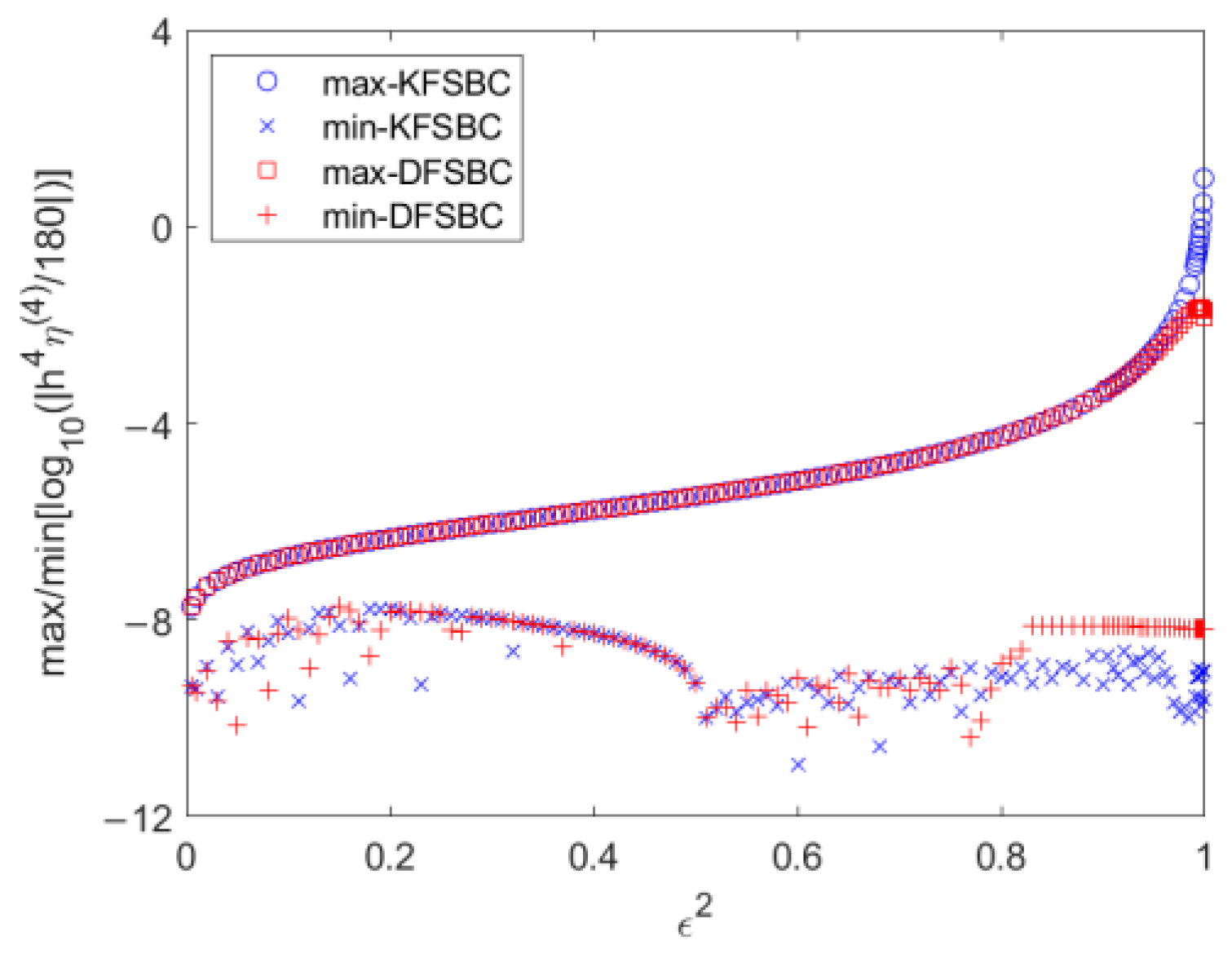
To indicate the possible global error of Simpson’s rule on integrating water surfaces using KFSBC or DFSBC, the maximum and minimum values of the absolute GErr at all positions kxj (j = 0, 1, …, N) are shown in Figure 1 for ε2 from 0.05 to 0.9999. The vertical axis indicates the value of the absolute GErr. The values of the absolute maximum GErrs using the water surfaces of KFSBC and DFSBC are equivalent and vary from −8 to −4 for ε2 < 0.8. For ε2 > 0.8, the values of both maximum absolute GErrs gradually become different, even up to 1 and −2 at the case of ε2 = 0.9999. The absolute GErrs of KFSBC are greater than those of DFSBC. The maximum absolute GErr for all cases occurs at the crest, and the minimum absolute GErr occurs near the zero water surface. The value of GErr depends on the fourth derivative of the water-level function at any point kx, as shown in the appendix. Equation (6) shows that the water surface is expressed by a sum of the cosine function. The cosine function has a recurrent fourth derivative. When kx = 0 on the crest, the fourth derivatives of all cosine functions are 1 so that the sum of the corresponding derivatives associated with positive coefficients, Bn, is larger than those at other positions. For the same reason, when kx is close to π/2 near the zero water level, the fourth derivatives of all cosine functions are approximated to zero so that the sum of the corresponding derivatives is minimum rather than at other positions.
Roundoff errors in floating-point numbers and propagated errors in the succeeding steps of Newton’s iteration are the minor error sources of the FSA. Double precision in all floating-point numbers is used in the calculation of the FSA to decrease the effects of round-off errors and propagated errors on the computational accuracy.
3.2. Comparisons of Accuracy with Three Previous Works
Various authors have formulated this problem using complex function theory, performed numerical computations, and revealed some interesting phenomena. Some results of the physical properties were tabulated by Cokelet [14], Williams [18], and Longuet-Higgins and Tanaka [53] to indicate the accuracy of their proposed methods. The agreement between such results and those presented here is a way to examine the accuracy of FSA.
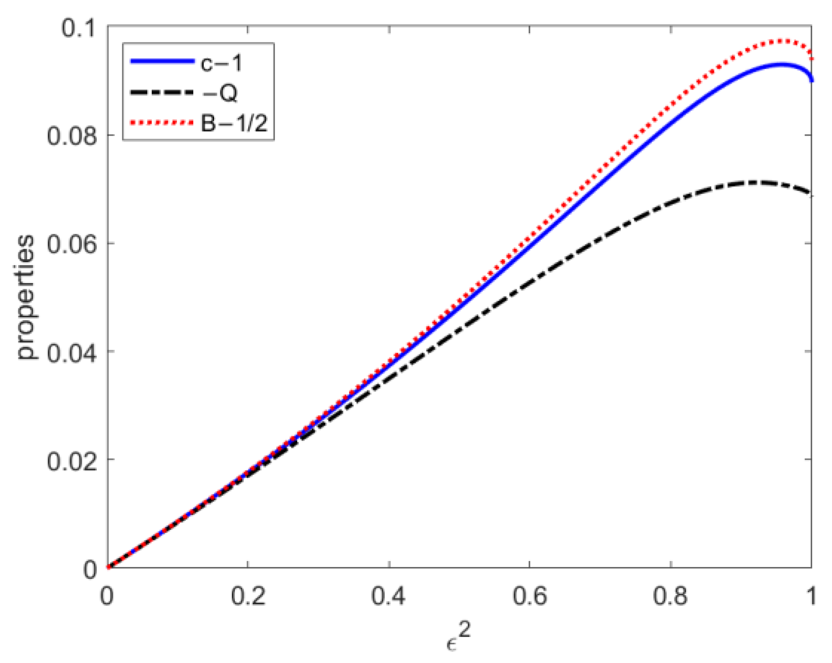
Some integral properties of waves, such as the mean momentum and energy and their respective fluxes, are of particular interest to hydraulicians and oceanographers. A known interesting result is that most physical quantities reach maximums ahead of the limiting wave. For example, the values of c, Q, and B obtained using FSA are shown in Figure 2 for the same scale for c − 1, −Q, and B − 0.5. The three physical quantities reach maxima at ε2 of around 0.92 to 0.96.
Table A0 of Cokelet [14], page 220, shows the wave amplitude, ka, squared speed, c2, and some physical properties at the parameter ε2 varying from 0.0 to 0.8 per 0.1 and from 0.81 to 1.0 per 0.01. Longuet-Higgins [55] derived various relations between the integral properties related to c, Q, B, etc.
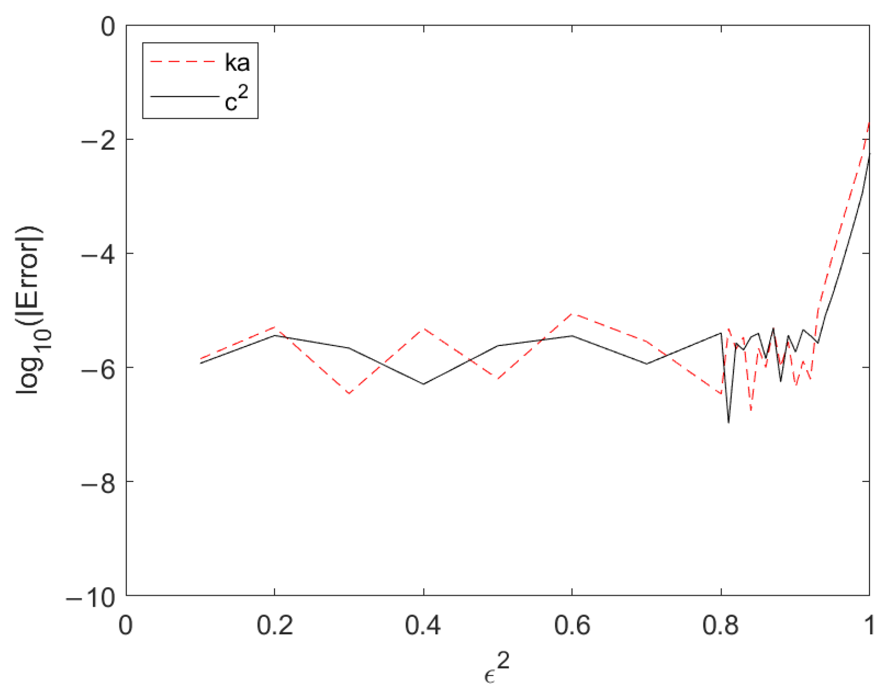
By the same values of ε2 in Cokelet [14], the differences between the present results and Cokelet [14] are indicated in Figure 3. The vertical axis of Figure 3 indicates the common logarithm of the absolute error between both results. The common logarithm being lower than −5 directs the error to the six-decimal digit. The common logarithms of ka and c2 greater than −5 occur after ε2 = 0.93 and 0.94, respectively. However, the common logarithms of other physical properties also greater than −5 occur together after ε2 = 0.80.
Table 7 of Williams [18] shows six physical properties of almost-limiting deep-water waves with the parameter ω defined as Equation (13). Table 2 shows a comparison between the results of Williams [18] and the FSA. The value of ω is very close to ε2 for these almost-limiting waves. Longuet-Higgins and Fox [26] regarded an intermediate zone of the flow in almost-limiting waves, whose scale was large in relation to the inner profile but small compared to the wave as a whole, to derive the phase velocity and several integral properties of almost-limiting waves.
Longuet-Higgins and Fox [26] considered a small expansion to express the small departure of some properties of an almost-limiting wave from those of the limiting form. The definition of such a small parameter is as follows.
For the limiting wave, is zero, and approaches zero for an almost-limiting wave. It is seen that both values of have tiny differences by less than 3 × 10⁻⁵ for eight cases. The differences between the values of wave steepness occur at five decimal places for the four bottom cases and at three decimal places for the top case. For the celerity, the FSA has differences at five or six decimal places for low almost-limiting waves but has differences at four decimal places for high almost-limiting waves.
Dyachenko et al. [32] obtained a very high accuracy for H/L and c for the limiting wave from simulations with quadruple and variable precisions of 0.1410633 and 1.0922851405. For the case of ω = 0.99924, H/L and c calculated by Williams [18] are more consistent with those of Dyachenko et al. [32] for the limiting wave than the present results. The H/L and c obtained using the FSA have relative errors related to Williams’ [18] values of 0.40% and 0.19%, respectively.
Table 3 shows a comparison of ak, , c, and R/l against the parameter ωT between Longuet-Higgins and Tanaka [53] and the current study. R is the radius of curvature at the wave crest, and l is a characteristic length defined by Longuet-Higgins and Fox [26]. For almost-limiting waves, Longuet-Higgins and Fox [26] examined the inner profile that is still rounded near the crest but with the flow approaching Stokes’s corner flow. The inner profile may be enveloped by an angled bilinear roof whose intersection is above the crest by a distance of l = q2/2g, where q is the particle speed at the crest in a reference frame that moves with the wave speed. Taking the second derivative of the surface profile expressed by Equations (2) and (3), respectively, yields two radiuses of curvature. The last two columns are R/l obtained using the FSA. For ωT < 0.9, the differences between both results for ak, ε’, and c are in the five decimal digits. For ωT > 0.9, the differences between the two results for ak, ε’, and c reach three decimal places, especially for ωT = 0.96. The difference of ε’ is less than 5 × 10⁻⁵, indicating that the fluid velocities at the crest obtained using both methods are very close.
The radius of curvature R on the crest obtained by Longuet-Higgins and Tanaka [53] converges to the value 5.15ε2 predicted in Longuet-Higgins and Fox [26]. The last two columns in Table 3 indicate different curvature radiuses obtained using the FSA and exceed that of Longuet-Higgins and Tanaka [53]. The radius of curvature obtained from the surface profile ηd is much greater than that from ηk, indicating that the surface profile ηd around the crest is flatter than ηk. A detailed discussion of the surface profile is introduced in the next subsection.
3.3. The Celerity of Almost-Limiting Waves
Drennan et al. [58] examined the extending and accelerating convergence of the Padé approximants for the celerity of the gravity waves (Schwartz [12]). Longuet-Higgins [59] developed an algorithm to avoid the lack of intrinsic convergence of the Stokes method. Hui and Tenti [60] derived a direct formulation with relatively low-order partial sums for accurate values for all wave properties, even for very high waves. This applies to the case of finite depth as well (see Drennan [61]) and may also be extended to include surface tension effects (see Drennan et al. [58]).
Lukomsky et al. [58] constructed two numerical algorithms using the truncated Fourier series method and the collocation method in a plane of independent spatial variables. The speed of steep gravity waves on their steepness using both accurate calculations shows that the point of the limiting steepness seems to be the maximum point A, not the breaking point. Lukomsky et al. [62,63] revealed a new branch of the spike wave that has a surface profile near the crest sharper than the profile of the Stokes wave of the same steepness. Murashige [64] showed the non-monotonic variation of wave speed with wave steepness using a linear sum of a relatively small number of singularities.
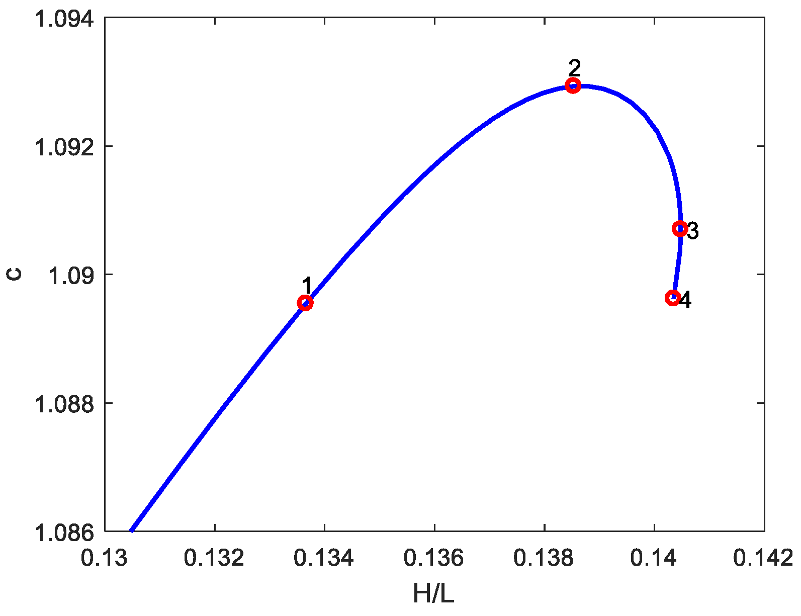
Figure 4, with four critical points marked by numbers from one to four, shows the wave phase speed of an almost-limiting surface wave versus its steepness obtained using the FSA. Point 2 is the maximum of the wave speed; point 3 is the limiting steepness, the relative minimum; and point 4 corresponds to the wave speed of the extremely limiting wave at ε2 = 0.99999. Point 1 is the other branch of almost-limiting wave with a wave speed similar to that of the limiting wave.
Table 4 lists the values of the wave speed and the corresponding steepness of four points. The FSA also shows a nonmonotonic variation of wave speed with wave steepness without a loop as that obtained by Tanaka [56] and Lukomsky et al. [62,63] for the almost-limiting waves.
Lushnikov et al. [35] developed a highly efficient method to compute the wave celerity of Stokes waves traveling on the free surface of deep water. Lushnikov et al. [35] fitted the simulation data for the ratio of celerity to wave height to obtain a regressive form.
where the fitting coefficients are α = 0.394794 ± 10−6, ω1 = 0.71430 ± 10−5, φ1 = 1.98059 ± 2 × 10⁻⁵, clim = 1.0922850485865375 ± 10−16, A = 0.12893 ± 5 × 10⁻⁵, and Hmax/λ = 0.141063483980 ± 10−12.
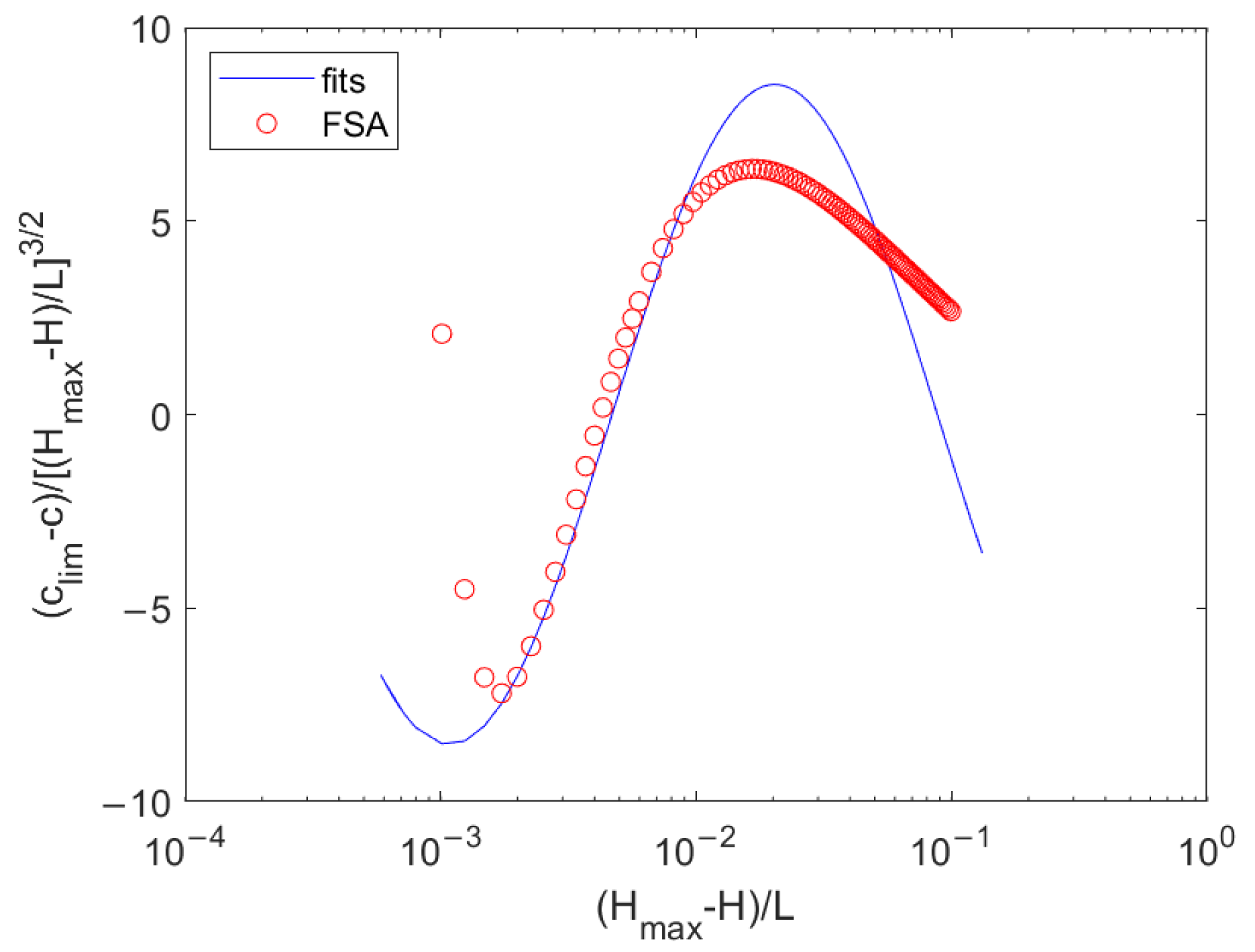
Using the clim and Hmax/L obtained by Lushnikov et al. [35], the values on the left side of Equation (18) obtained using the FSA and the fits on the right side of Equation (18) are shown in Figure 5. Figure 5 indicates a good agreement between the obtained ratios and the fits for the values of (Hmax − H)/L within 0.002 and 0.007 but gradually large differences for the values of (Hmax − H)/L less than 0.002. The result indicates that the FSA has a low accuracy, as the wave speed deviates clearly from that of Lushnikov et al. [35] for almost-limiting waves. The inaccuracy may result from the fact that the FSA is incapable of simultaneous satisfaction with KFSBC and DFSBC near the crest.
3.4. The Angled Crest and Inner Wave Profile
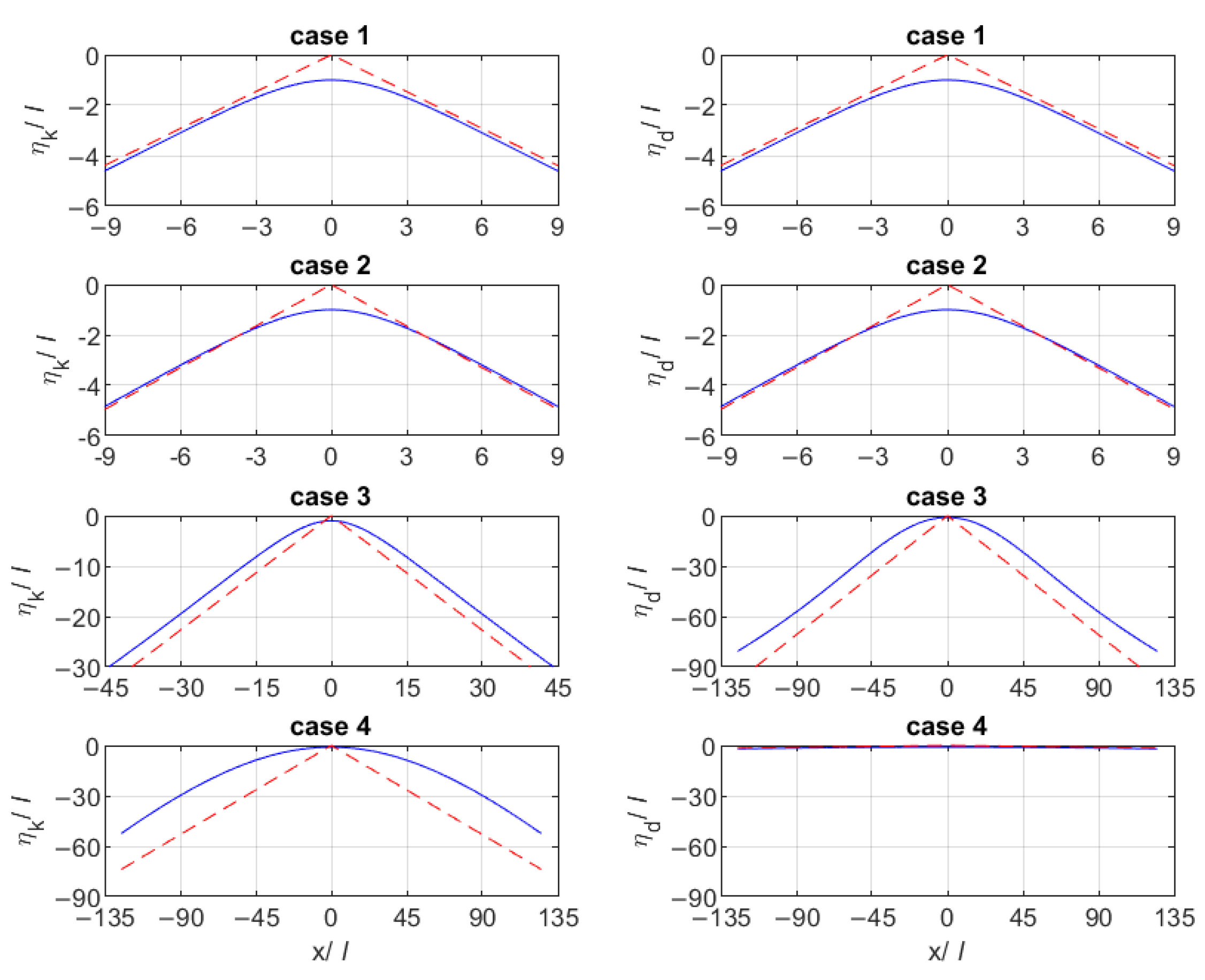
The values of l for the four cases of Table 4 are 4.7639 × 10⁻², 1.8066 × 10⁻², 8.0094 × 10⁻⁴, and 3.9962 × 10⁻⁶, respectively. When the coefficients Bn (n = 1, …, N), c, Q, and B are determined, the inner profile at any position can be calculated using Equations (6) and (7), respectively. The results are denoted by ηk and ηd. The inner wave profiles for the four cases are shown in Figure 6, of which the angled bilinear roof is denoted by dashed lines.
For case 1 and case 2, both inner profiles ηk and ηd are below the bilinear roof with an inner angle of 127.94°, 127.94°, 122.32°, 122.37°, respectively. For case 3, the inner angles of the bilinear roof of ηk and ηd are slightly different, being 105.68° and 103.57°. However, the inner angles of the bilinear roof of ηk and ηd are significantly different, being 118.94° and 178.61°, respectively, for case 4. Both bilinear roofs are below the crest of the inner profiles. The summits are very close to the crest of the inner profiles due to a very small l.
An interesting difference between the inner angle of the bilinear roof of ηk and ηd for case 4 shows that ηk keeps an angled inner profile, but ηd is flat. The slope at the crest is the first derivative of the inner profile, as indicated by Equations (A1) and (A10) at x = 0 in Appendix A. The vertical component of the particle velocity at the crest is always zero for the zero sine function. When the almost-limiting wave occurs, the horizontal component of the particle velocity at the crest approaches zero. For the limiting wave, Equation (A1) shows a singular limit due to the condition of zero being divided by zero. In this case, L’Hôpital’s rule can be applied to convert the indeterminate limit to an expression that can be evaluated by substitution. The substitution is a form of taking the derivative of both the v(x, η(x)) and u(x, η(x)) functions with respect to x, respectively, to have
where v(0, η(0)) = ux(0, η(0)) = 0, and vx(0, η(0)) = uy(0, η(0)). Thus, ηx(0) = ±1, implying that the inner angle at the crest of the limiting wave is 90°. Satisfying the kinematic properties of the particle along the surface streamline at the crest of a limiting wave, Rankine [65] and Havelock [66] proved that the wave begins to break when the two slopes of the crest meet at right angles. Equation (19) is consistent with this conclusion.
The slope of the surface profile at the crest using DFSBC is
where u(0, η(0)) = v(0, η(0)) = 0 for the limiting wave. Therefore, Equation (20) shows that the slope of the surface profile on the crest is always zero, which is different from that using Equation (19).
Stokes [5] showed that the limiting Stokes wave has a singularity in the form of a sharp angle of 2π/3 radians on the crest, indicating that its slope of the surface profile is 30°. Except for the Stokes 2/3 power-law singularity, Grant [6] and Tanveer [10] showed that the only possible singularity in the finite complex upper half-plane of the physical sheet of the Riemann surface is of a square root type. The formation of a 2/3 power-law singularity of the limiting Stokes wave is verified theoretically and numerically by Lushnikov [67] as a combination of an infinite number of square-root singularities from different sheets of the Riemann surface as the branch point approaches zero.
In previous numerical calculations of limiting waves [15,22], the conformal transformation was used to map a half-strip complex potential plane to a fluid domain of an infinite depth of a physical plane, and its possible solution was assumed to be a combination of a 2/3 power term or supplemented by an irrational power term and an analytic series based on the Stokes 2/3 power law singularity or Grant’s law singularity for the limiting wave. These calculations, of course, showed that the crested angle is close to 2π/3 radians. For example, Maklakov [23] applied the technique of Longuet-Higgins and Fox [26] to obtain the slope of the wave profile on the crest of 30.3787°. The value is in good agreement with the calculations of Chandler and Graham [25] who accurately calculated a very steep wave on deep water. The inner crest angles of the limiting Stokes wave at different depths, given by the HAM approach, range from 119.2° to 120.2°, which are very close to the theoretical value of 120° (Zhong and Liao [43]).
Unlike previous studies that were based on the complex potential plane, the formulation of the FSA is based on the physical plane. The boundary conditions on the free surface, Equations (6) and (7), contribute to FSA in an implicit form of x and η(x), which is unknown and changes with x. Therefore, the coefficient of the cos term of the FSA is not simply an unknown value but is related to x. These unknown variables in the FSA can be solved using KFSBC and DFSBC at the same time. Zhao et al. [47] pointed out that using different series terms to represent the wave profile and the velocity potential can simultaneously reduce the residuals of KFSBC and DFSBC for large waves. The improvement in KFSBC is quite significant compared to DFSBC. Because the wave profile is assumed to be a Fourier cosine series, the slope always remains zero at the crest, so that the residual values of KFSBC and DFSBC are always zero at the crest. However, the residual values of KFSBC and DFSBC at different positions vibrate and attenuate from the crest to the trough, and the maximum value occurs at the point adjacent to the crest (see Figure 8 of Zhao et al. [47]). Lukomsky et al. [63] used the Fourier series with hundreds of terms to represent the velocity potential and the wave profile, of which the harmonics were obtained by using kinematic and dynamic boundary conditions alone recursively. The wave profile is not assumed to be a Fourier cosine series in the FSA, which is the main difference from Zhao et al. [47] and Lukomsky et al. [63].
The possible Fourier solution on the complex plane is in an explicit form of only potential; additionally, the value of the conjugate stream function at the surface is set to zero. While all coefficients of the Fourier series are unknown constants which can be solved by using the DFSBC condition, Zhong and Liao [43] obtained all coefficients of thousands of truncated terms of a Fourier series for the limiting wave on deep water using HAM. In terms of methodology, the solution of FSA on the physical plane will be more difficult than the Fourier series solution on the complex variable plane.
3.5. Difference between Hk and Hd at All Interpolated Points
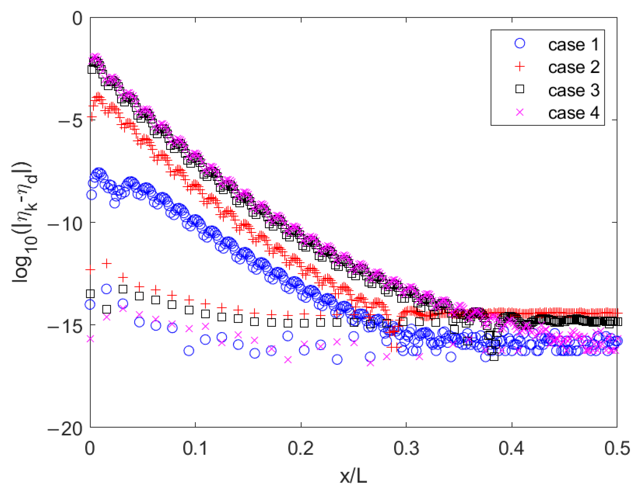
In order to illustrate the difference in surface profiles based on KFSBC and DFSBC, the fine surface profiles are interpolated at 320 equally spaced points over a half-wave length and shown in Figure 7 for the four almost-limiting waves. Figure 7 clearly shows that the differences between ηk and ηd near the crest are much greater than those near the trough which are less than 10−13. The differences at the specified points in the FSA, which are the originally spaced intervals, k△xj = jπ/32 (j = 0, 1, …, 32), are less than 10−11 for the four cases. Both ηk and ηd at such specified points are required to satisfy the KFSBC and DFSBC together so that the differences are lower than the specified tolerance, 10−10.
The means of ηk and ηd at the 320 equally spaced points and the difference in the corresponding potential for the four cases are listed in Table 5. The zero mean of a surface profile is one of the governing equations, Equation (10), of the FSA, so that the mean of the obtained surface elevations at the original 32 equally spaced points is less than 10−10. However, the means of ηk and ηd for the four cases in Table 5 are from 10−6 to 10−4, which are much greater than the specified tolerance. The maximum difference of ηk and ηd reaches 10−2 for case 4.
The potentials of the 320 equally spaced points using KFSBC for cases 1–3 exceed those of the 32 equally spaced points. On the contrary, the potential of the 320 equally spaced points using KFSBC is less than that of the 32 equally spaced points. However, the potentials of the 320 equally spaced points using DFSBC for the four cases are greater than those of the 32 equally spaced points. All means and are positive and increase the potentials except the negative for case 4.
From the above discussion, an inference conjectures that keeping some leading N terms from the original form of an infinite series cannot satisfy KFSBC and DFSBC together at the surface points around the crest. In other words, Equations (6) and (7) cannot be satisfied together at the surface points around the crest, even for the almost-limiting waves, not to mention the limiting wave.
3.6. The Position of Singularity
Stokes [5] first demonstrated that the singularity that occurs at the crest of the steepest possible water wave at an infinite depth has a 2/3 power-law singularity forming a 120° angle on the crest. Grant [6] showed that, for any wave away from the steepest configuration, the singularity moves into the complex plane and is of a square-root order. Grant [6] conjectured that as the limiting wave approaches, other singularities must coalesce at the crest to cancel the square-root behavior. Lushnikov [67] differentiated the location of the branch point of singularities that coalesce as the Stokes limiting wave approaches.
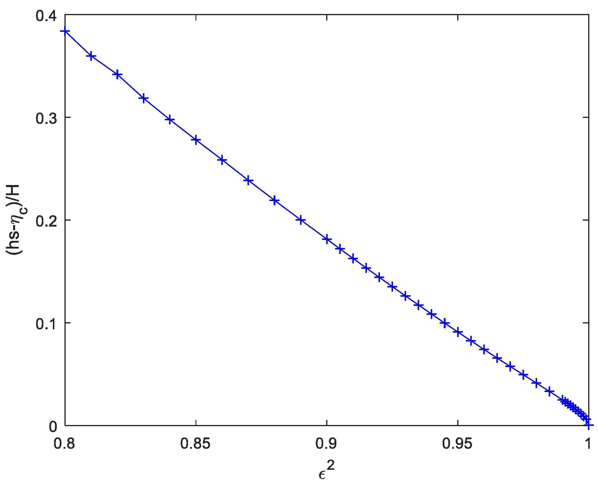
For almost-limiting waves, the fluid velocity at the crest has a zero vertical component and a nonzero but negative horizontal component, that is, v(0, η(0)) = 0 and u(0, η(0)) < 0. The location of singularities for the almost-limiting waves is exactly over the crest by a distance at which the fluid velocity in a complex conjugate domain is zero in the moving reference frame. For a limiting wave, the FSA can calculate the fluid velocity at any position when Bn (n = 1, …, N) is determined. The location of the singularity at u(0, hs) = 0 can be determined iteratively by using the FSA using the Newton method. Figure 8 shows the heights of the singularity exactly over the crest against ε2 using the FSA.
When a wave is far from the limiting wave (ε2→0.8), the height of singularity, hs, is removed from the crest. When a wave is approaching the limiting wave (ε2→1), the height of singularity, hs, advances on the crest to have zero hs − ηc. The singularity closely coalesces the physical domain and makes the condition of ill-varied Newton’s iterations. The singularities coalescing as the Stokes limit wave should be well understood. This is another key to exactly express the governing equations for the almost-limiting waves, even for the limiting wave.
4. Conclusions
The FSA was evaluated as a valid collation method for the classic problem of a permanent gravity wave propagating at all water depths. The FSA is commonly applied to study the physical properties of small, almost-limiting waves on deep water to expand its applicability. We evaluate the accuracy of the FSA for almost-limiting gravity waves and explore the reasons for its shortcomings in this study.
Some physical properties calculated using the FSA for all possible Stokes waves are compared with those of Cokelet [14], Williams [18], and Longuet-Higgins and Tanaka [53] based on the same corresponding parameters. The celerity of the almost-limiting wave is compared with that obtained using the empirical formula of Lushnikov et al. [35]. These comparisons indicate slight differences, which are at five or six decimal places, of the physical properties of almost-limiting waves between the present results and other works. Therefore, the FSA can also present the physical properties of gravity waves that have a maximum value before wave breaking, as studied in the past.
However, we found that the surface water levels at all locations obtained using KFSBC and DBSBC for four selected almost-limiting waves are significantly different. The difference is much greater near the crest than at the trough. The difference shows different angled crests and inner profiles. It can be conjectured from the results that KFSBC and DFSBC cannot be satisfied at the same time when the FSA has finite harmonics. This would explain why the harmonic terms in the FSA cannot exceed 40 for almost-limiting waves, the harmonic terms calculated in previous studies are also limited, and the results have convergence problems with the number of terms of a series. The inaccuracy of the FSA without a suitable form in presenting singularities of order 1/2 or 2/3 for the almost-limiting waves results from the height of the singularity approaching the crest. Perhaps this problem may be caused by the truncation of finite terms in the original infinite-series solution. Clamond’s RCW (renormalized cnoidal wave) method [68] of converting infinite series into a simple Fourier–Padé form may be a good inspiration for improving the FSA in the future.
Author Contributions
Conceptualization, Y.-Y.C.; methodology, H.-K.C.; software, H.-K.C.; writing—original draft preparation, H.-K.C.; writing—review and editing, H.-K.C. and H.-K.C. All authors have read and agreed to the published version of the manuscript.
Funding
This research received no external funding.
Data Availability Statement
No new data were created or analyzed in this study.
Conflicts of Interest
The authors declare no conflicts of interest.
Appendix A
The fourth leading derivatives of the wave profile can be derived using KFSBC and DFSBC, Equations (2) and (3), respectively. The general solution to the present problem is given by Equation (5).
Appendix A.1. The Slope of the Surface Profile Using KFSBC
Taking the first derivative to Equation (2), KFSBC, with respect to x, yields the slope of the wave profile at any point as
where
and
Taking the derivative of Equation (A1) gives the second derivative
where the subscripts x and y denote the partial derivative with respect to x and y. The next two derivatives are the following.
where
The results can be easily derived using symbolic operations software, such as Maple or Mathematica. The radius of curvature mentioned in Section 3.2 is defined by
Equation (A1) shows a zero slope at the crest due to v(0, η(0)) = 0. Inserting v(0, η(0)) = 0 and ηx(0) = 0 in Equation (A4) yields ηxx(0) = vx/u. Therefore, the radius of curvature at the crest can be simply expressed by
Appendix A.2. The Slope of the Surface Profile Using DFSBC
Taking the leading fourth derivative of Equation (3), DFSBC, with respect to x, yields the slope of the wave profile at any point of DFSBC
and
Taking the derivative of u with respect to x visually shows ux(0, η(0)) = 0. Associated with v(0, η(0)) = 0, the slope of the surface profile on the crest is also zero using Equation (A10). The radius of curvature at the crest leads to a simple result from
Both Equations (A9) and (A15) show the radius of curvature at the crest in different forms, of which the values are listed in Table 3 for some almost-limiting waves.
References
- Stokes, G.G. On the theory of oscillatory waves. Trans. Cambr. Phil. Soc. 1847, 8, 441–455. [Google Scholar]
- Skjelbreia, L.; Hendrickson, J. Fifth order gravity wave theory. In Coastal Engineering Proceedings; ASCE: Reston, Virginia, 1960; pp. 184–196. [Google Scholar]
- Isobe, M.; Nishimura, H.; Horikawa, K. Expressions of Perturbation Solutions for Conservative Waves by Using Wave Height; Japan Society of Civil Engineers: Fokuoka, Japan, 1978; pp. 760–761. (In Japanese) [Google Scholar]
- Fenton, J.D. A fifth-order Stokes theory for steady waves. J. Waterw. Port Coast. Ocean Eng. 1985, 111, 216–234. [Google Scholar] [CrossRef]
- Stokes, G.G. Supplement to a paper on the theory of oscillatory waves. Math. Phys. Pap. 1880, 1, 314–326. [Google Scholar]
- Grant, M.A. The singularity at the crest of a finite amplitude progressive Stokes wave. J. Fluid Mech. 1973, 59, 257–262. [Google Scholar] [CrossRef]
- Toland, J.F. On the existence of a wave of greatest height and Stokes’s conjecture. Proc. R. Soc. Lond. A 1978, 363, 469–485. [Google Scholar]
- Pelinovsky, D.; Stepanyants, Y. Convergence of Petviashvili’s iteration method for numerical approximation of stationary solutions of nonlinear wave equations. SIAM J. Numer. Anal. 2004, 42, 1110–1127. [Google Scholar] [CrossRef]
- Amick, C.J.; Fraenkel, L.E.; Toland, J.F. On the stokes conjecture for the wave of extreme form. Acta Math. 1982, 148, 193–214. [Google Scholar] [CrossRef]
- Tanveer, S. Singularities in water waves and Rayleigh-Taylor instability. Proc. R. Soc. Lond. A 1991, 435, 137–158. [Google Scholar]
- Yamada, H. Highest waves of permanent type on the surface of deep water. Appl. Mech. Res. Rep. Kyushu Univ. 1957, 5, 37–52. [Google Scholar]
- Schwartz, L.W. Computer extension and analytic continuation of Stokes’ expansion for gravity waves. J. Fluid Mech. 1974, 62, 553–578. [Google Scholar] [CrossRef]
- Byatt-Smith, J.G.B.; Longuet-Higgins, M.S. On the speed and profile of steep solitary waves. Proc. R. Soc. Lond. A 1976, 350, 175–189. [Google Scholar]
- Cokelet, E.D. Steep gravity waves in water of arbitrary uniform depth. Philos. Trans. R. Soc. Lond. A 1977, 286, 183–230. [Google Scholar]
- Chen, B.; Saffman, P. Numerical evidence for the existence of new types of gravity waves of permanent form on deep water. Stud. Appl. Math. 1980, 62, 1–21. [Google Scholar] [CrossRef]
- Williams, J.M. Limiting gravity waves in water of finite depth. Philos. Trans. R. Soc. Lond. A 1981, 302, 139–188. [Google Scholar]
- Williams, J.M. Near-limiting gravity waves in water of finite depth. Philos. Trans. R. Soc. Lond. A 1985, 314, 353–377. [Google Scholar]
- Schwartz, L.W.; Fenton, J.D. Strongly nonlinear waves. Annu. Rev. Fluid Mech. 1982, 14, 39–60. [Google Scholar] [CrossRef]
- Hunter, J.K.; Vandenbroeck, J.M. Accurate computations for steep solitary waves. J. Fluid Mech. 1983, 136, 63–71. [Google Scholar] [CrossRef]
- Klopman, G. A note on integral properties of periodic gravity waves in the case of a non-zero mean Eulerian velocity. J. Fluid Mech. 1990, 211, 609–615. [Google Scholar] [CrossRef]
- Karabut, E.A. An approximation for the highest gravity waves on water of finite depth. J. Fluid Mech. 1998, 372, 45–70. [Google Scholar] [CrossRef]
- Rienecker, M.M.; Fenton, J.D. A Fourier approximation method for steady water waves. J. Fluid Mech. 1981, 104, 119–137. [Google Scholar] [CrossRef]
- Maklakov, D.V. Almost-highest gravity waves on water of finite depth. Eur. J. Appl. Math. 2002, 13, 67–93. [Google Scholar] [CrossRef]
- Clamond, D.; Dutykh, D. Accurate fast computation of steady two-dimensional surface gravity waves in arbitrary depth. J. Fluid Mech. 2018, 844, 491–518. [Google Scholar] [CrossRef]
- Chandler, G.A.; Graham, I.G. On the crest instabilities of steep surface waves. SIAM J. Numer. Anal. 1993, 30, 1041–1065. [Google Scholar] [CrossRef]
- Longuet-Higgins, M.S.; Fox, M.J.H. Theory of the almost-highest wave. Part 2. Matching and analytic extension. J. Fluid Mech. 1978, 85, 769–786. [Google Scholar] [CrossRef]
- Olfe, D.B.; Rottman, J.W. Some new highest-wave solutions for deep-water waves of permanent form. J. Fluid Mech. 1980, 100, 801–810. [Google Scholar] [CrossRef]
- Vanden-Broeck, J.M. Steep gravity waves: Havelock’s method revisited. Phys. Fluids 1986, 29, 3084–3085. [Google Scholar] [CrossRef]
- Zakharov, V.E. Modulation instability: The beginning. Physical D 2009, 238, 540–548. [Google Scholar] [CrossRef]
- Graves-Morris, P.R. A review of Padé methods for the acceleration of convergence of a sequence of vectors. Appl. Numer. Math. 1994, 15, 153–174. [Google Scholar] [CrossRef]
- Dyachenko, S.A.; Lushnikov, P.M.; Korotkevich, A.O. The complex singularity of a Stokes wave. J. Exp. Theor. Phys. Lett. 2014, 98, 675–679. [Google Scholar] [CrossRef]
- Dyachenko, S.A.; Lushnikov, P.M.; Korotkevich, A.O. Branch cuts of Stokes wave on deep water. Part I: Numerical solution and Padé approximation. Stud. Appl. Math. 2016, 137, 419–472. [Google Scholar] [CrossRef]
- Lushnikov, P.M.; Dyachenko, S.A.; Korotkevich, A.O. Branch cut singularity of Stokes wave on deep water. In Proceedings of the Ninth IMACS International Conference on Nonlinear Evolution Equations and Wave Phenomena, Athens, GA, USA, 1–4 April 2015; University of Georgia: Athens, GA, USA, 2015. [Google Scholar]
- Crew, S.C.; Trinh, P.H. New singularities for Stokes waves. J. Fluid Mech. 2016, 798, 256–283. [Google Scholar] [CrossRef]
- Lushnikov, P.M.; Dyachenko, S.A.; Silantyev, D.A. New conformal mapping for adaptive resolving of the complex singularities of Stokes wave. Proc. R. Soc. Lond. A 2017, 473, 20170198. [Google Scholar] [CrossRef] [PubMed]
- Clamond, D. Note on the velocity and related fields of steady irrotational two-dimensional surface gravity waves. Philos. Trans. R. Soc. Lond. A 2012, 370, 1572–1586. [Google Scholar] [CrossRef] [PubMed]
- Constantin, A. Nonlinear water waves. Philos. Trans. R. Soc. Lond. A 2012, 370, 1501–1504. [Google Scholar] [CrossRef]
- Vanden-Broeck, J.M.; Schwartz, L.W. Numerical computation of steep gravity waves in shallow water. Phys. Fluids 1979, 22, 1868–1871. [Google Scholar] [CrossRef]
- Clamond, D.; Dutykh, D. Fast accurate computation of the fully nonlinear solitary surface gravity waves. Comput. Fluids 2013, 84, 35–38. [Google Scholar] [CrossRef]
- Dutykh, D.; Clamond, D. Efficient computation of steady solitary gravity waves. Wave Motion 2014, 51, 86–99. [Google Scholar] [CrossRef]
- Clamond, D.; Dutykh, D.; Durán, A. A plethora of generalised solitary gravity-capillary water waves. J. Fluid Mech. 2015, 784, 664–680. [Google Scholar] [CrossRef]
- Dutykh, D.; Clamond, D.; Durán, A. Efficient computation of capillary-gravity generalised solitary waves. Wave Motion 2016, 65, 1–16. [Google Scholar] [CrossRef]
- Zhong, X.; Liao, S. On the limiting Stokes wave of extreme height in arbitrary water depth. J. Fluid Mech. 2018, 843, 653–679. [Google Scholar] [CrossRef]
- Hansen, J.B.; Svendsen, I.A. Regular Waves in Shoaling Water: Experimental Data; series paper no. 21; Institute of Hydrodynamics and Hydraulic Engineering, Technical University of Denmark: Kongens Lyngby, Denmark, 1979. [Google Scholar]
- Dean, R.G.; Dalrymple, R.A. Water Wave Mechanics for Engineers and Scientists; World Scientific Publishing Co., Inc.: Singapore, 1991. [Google Scholar]
- Vivanco, I.; Cartwright, B.; Ledesma Araujo, A.; Gordillo, L.; Marin, J.F. Generation of Gravity Waves by Pedal-Wavemakers. Fluids 2021, 6, 222. [Google Scholar] [CrossRef]
- Zhao, H.J.; Song, Z.Y.; Li, L.; Kong, J. On the Fourier approximation method for steady water waves. Acta Oceanol. Sin. 2014, 33, 37–47. [Google Scholar] [CrossRef]
- Chang, H.K. Shoaling of nonlinear waves over a gently sloping bottom. J. Chin. Inst. Civ. Hydraul. Eng. 1999, 11, 175–180. (In Chinese) [Google Scholar]
- Eldrup, M.R.; Andersen, L.T. Numerical study on regular wave shoaling, de-shoaling and decomposition of free/bound waves on gentle and steep foreshores. J. Mar. Sci. Eng. 2020, 8, 334. [Google Scholar] [CrossRef]
- Chang, H.K.; Chen, Y.Y.; Liou, J.C. Particle trajectories of nonlinear gravity waves in deep water. Ocean Eng. 2009, 36, 324–329. [Google Scholar] [CrossRef]
- Chang, H.K.; Liou, J.C.; Su, M.Y. Particle trajectory and mass transport of finite-amplitude waves in water of uniform depth. Eur. J. Mech. B Fluids 2007, 26, 385–403. [Google Scholar] [CrossRef]
- Longuet-Higgins, M.S. Lagrangian moments and mass transport in Stokes waves. J. Fluid Mech. 1987, 179, 547–555. [Google Scholar] [CrossRef]
- Longuet-Higgins, M.S.; Tanaka, M. On the crest instabilities of steep surface waves. J. Fluid Mech. 1997, 336, 51–68. [Google Scholar] [CrossRef]
- Longuet-Higgins, M.S.; Fenton, J.D. On the mass, momentum, energy, and circulation of a solitary wave II. Proc. R. Soc. Lond. A 1974, 340, 471–493. [Google Scholar]
- Longuet-Higgins, M.S. Integral properties of periodic gravity waves of finite amplitude. Proc. R. Soc. Ser. A 1975, 342, 157–174. [Google Scholar]
- Tanaka, M. The stability of steep gravity waves. J. Phys. Soc. Jpn. 1983, 52, 3047–3055. [Google Scholar] [CrossRef]
- Gerald, C.F.; Wheatley, P.O. Applied Numerical Analysis, 5th ed.; Pearson Education, Inc.: Singapore, 2004; pp. 364–366. [Google Scholar]
- Drennan, W.M.; Hui, W.H.; Tenti, G. Accurate calculations of stokes water waves of large amplitude. J. Appl. Math. Phys. (ZAMP) 1992, 43, 367–384. [Google Scholar] [CrossRef]
- Longuet-Higgins, M.S. Limiting forms for capillary-gravity waves. J. Fluid Mech. 1988, 194, 351–375. [Google Scholar] [CrossRef]
- Hui, W.H.; Tenti, G. A new approach to steady flows with free surfaces. J. Appl. Math. Phys. (ZAMP) 1982, 33, 569–589. [Google Scholar] [CrossRef]
- Drennan, W.M. Accurate Calculations of the Stokes Water Wave. Ph.D. Dissertation, University of Waterloo, Waterloo, ON, Canada, 1988. [Google Scholar]
- Lukomsky, V.P.; Gandzha, I.S.; Lukomsky, D.V. Steep sharp-crested gravity waves on deep water. Phys. Rev. Lett. 2002, 89, 164502. [Google Scholar] [CrossRef] [PubMed]
- Lukomsky, V.P.; Gandzha, I.S.; Lukomsky, D.V. Computational analysis of the almost-highest waves on deep water. Comput. Phys. Commun. 2002, 147, 548–551. [Google Scholar] [CrossRef]
- Murashige, S. Davies’ surface condition and singularities of deep water waves. J. Eng. Math. 2014, 85, 19–34. [Google Scholar] [CrossRef]
- Rankine, W.J.M. Supplement to a paper on stream-lines. Philos. Mag. 1865, 4, 25–28. [Google Scholar] [CrossRef]
- Havelock, T.H. Periodic irrotational waves of finite height. Proc. R. Soc. Lond. A 1919, 95, 38–51. [Google Scholar]
- Lushnikov, P.M. Structure and location of branch point singularities for Stokes waves on deep water. J. Fluid. Mech. 2016, 800, 557–594. [Google Scholar] [CrossRef]
- Clamond, D. Cnoidal-type surface waves in deep water. J. Fluid Mech. 2003, 489, 101–120. [Google Scholar] [CrossRef]
Figure 1.
The maximum and minimum values of the absolute global errors of Simpson’s rule for integrating water surfaces against ε2.
Figure 1.
The maximum and minimum values of the absolute global errors of Simpson’s rule for integrating water surfaces against ε2.

Figure 2.
Phase speed, the value of the stream function on the surface, and Bernoulli’s constant against ε2.
Figure 2.
Phase speed, the value of the stream function on the surface, and Bernoulli’s constant against ε2.

Figure 3.
The difference between the Cokelet results [14] and those of today for some physical quantities against ε2.
Figure 3.
The difference between the Cokelet results [14] and those of today for some physical quantities against ε2.

Figure 4.
The celerity of almost-limiting waves against wave steepness and four critical points marked by numbers from one to four.
Figure 4.
The celerity of almost-limiting waves against wave steepness and four critical points marked by numbers from one to four.

Figure 5.
The ratio of wave speed to wave steepness and fits obtained by Lushnikov et al. [35].
Figure 5.
The ratio of wave speed to wave steepness and fits obtained by Lushnikov et al. [35].

Figure 6.
Inner wave profile for four cases (solid line: ηk and ηd obtained using KFSBC or DFSBC; dashed line: linear bilinear fitting lines for outer profiles).
Figure 6.
Inner wave profile for four cases (solid line: ηk and ηd obtained using KFSBC or DFSBC; dashed line: linear bilinear fitting lines for outer profiles).

Figure 7.
Difference between surface elevation at 320 equally spaced points based on KFSBC and DFSBC.
Figure 7.
Difference between surface elevation at 320 equally spaced points based on KFSBC and DFSBC.

Figure 8.
Heights of the singularity exactly over the crest against ε2.


Table 1.
Convergence test of the FSA for Stokes waves on deep water.
| N | Max (Tol) | H/L | c | −Q | B |
|---|---|---|---|---|---|
| 8 | 1.11 × 10⁻¹⁶ | 0.139112 | 1.094930 | 0.065092 | 0.601168 |
| 16 | 4.44 × 10⁻¹⁶ | 0.139651 | 1.091030 | 0.067966 | 0.595586 |
| 24 | 3.33 × 10⁻¹⁶ | 0.140077 | 1.091465 | 0.069172 | 0.595821 |
| 32 | 6.77 × 10⁻¹⁶ | 0.140262 | 1.091847 | 0.069663 | 0.596157 |
| 40 | 4.70 × 10⁻⁸ | 0.140339 | 1.092044 | 0.069868 | 0.596338 |
Table 2.
Comparison of Williams [18] and the present results for some physical quantities.
Table 2.
Comparison of Williams [18] and the present results for some physical quantities.
| ω | H/L | c | ||||
|---|---|---|---|---|---|---|
| Williams | FSA | Williams | FSA | Williams | FSA | |
| 0.99924 | 0.01602 | 0.01599 | 0.141020 | 0.140452 | 1.092270 | 1.090219 |
| 0.99648 | 0.03440 | 0.03442 | 0.140867 | 0.140473 | 1.092260 | 1.090923 |
| 0.99444 | 0.04327 | 0.04326 | 0.140757 | 0.140439 | 1.092290 | 1.091228 |
| 0.98396 | 0.07347 | 0.07348 | 0.140245 | 0.140120 | 1.092488 | 1.092117 |
| 0.96023 | 0.11566 | 0.11566 | 0.139179 | 0.139161 | 1.092913 | 1.092864 |
| 0.94990 | 0.12978 | 0.12978 | 0.138707 | 0.138700 | 1.092950 | 1.092932 |
| 0.94044 | 0.14146 | 0.14146 | 0.138262 | 0.138260 | 1.092898 | 1.092892 |
| 0.92976 | 0.15358 | 0.15357 | 0.137743 | 0.137742 | 1.092748 | 1.092745 |
Table 3.
Comparison of Longuet-Higgins and Tanaka (LT) [53] and the present results against ωT for some physical quantities.
Table 3.
Comparison of Longuet-Higgins and Tanaka (LT) [53] and the present results against ωT for some physical quantities.
| ωT | ak | ε’ | c | R/l | |||||
|---|---|---|---|---|---|---|---|---|---|
| LT [53] | FSA | LT [53] | FSA | LT [53] | FSA | LT [53] | ηk | ηd | |
| 0.80 | 0.42674 | 0.42674 | 0.18858 | 0.18858 | 1.09157 | 1.09157 | 5.3274 | 5.3279 | 5.3322 |
| 0.82 | 0.43022 | 0.43021 | 0.16974 | 0.16974 | 1.09235 | 1.09235 | 5.2869 | 5.2889 | 5.3060 |
| 0.84 | 0.43312 | 0.43311 | 0.15086 | 0.15086 | 1.09279 | 1.09279 | 5.2529 | 5.2637 | 5.3208 |
| 0.86 | 0.43551 | 0.43550 | 0.13196 | 0.13196 | 1.09295 | 1.09293 | 5.2248 | 5.2635 | 5.4371 |
| 0.88 | 0.43749 | 0.43743 | 0.11307 | 0.11306 | 1.09289 | 1.09284 | 5.2021 | 5.3181 | 5.7719 |
| 0. 90 | 0.43912 | 0.43896 | 0.09419 | 0.09417 | 1.09272 | 1.09257 | 5.1843 | 5.4863 | 6.5609 |
| 0.92 | 0.44047 | 0.44011 | 0.07533 | 0.07530 | 1.09251 | 1.09216 | 5.1711 | 5.8773 | 8.3184 |
| 0.94 | 0.44158 | 0.44089 | 0.05649 | 0.05644 | 1.09235 | 1.09165 | 5.1618 | 6.7243 | 12.478 |
| 0.96 | 0.44244 | 0.44128 | 0.03766 | 0.03761 | 1.09228 | 1.09104 | 5.1560 | 8.6961 | 24.772 |
Table 4.
Wave steepness, ε2, and celerity for four critical points.
| Case | ε2 | H/L | c |
|---|---|---|---|
| 1 | 0.890 | 0.1343843 | 1.0902735 |
| 2 | 0.955 | 0.1385325 | 1.0929274 |
| 3 | 0.998 | 0.1404800 | 1.0906989 |
| 4 | 0.99999 | 0.1403509 | 1.0896230 |
Table 5.
Means of ηk and ηd at the 320 equally spaced points and corresponding maximum difference and potential energy (PE) compared to those at the 32 equally spaced points.
Table 5.
Means of ηk and ηd at the 320 equally spaced points and corresponding maximum difference and potential energy (PE) compared to those at the 32 equally spaced points.
| Case | PE32 − (PE320)k | PE32 − (PE320)d | |||
|---|---|---|---|---|---|
| 1 | 3.5183 × 10⁻⁶ | 3.5207 × 10⁻⁶ | 4.3521 × 10⁻⁷ | −2.2756 × 10⁻⁶ | −2.2770 × 10⁻⁶ |
| 2 | 3.6374 × 10⁻⁵ | 3.7892 × 10⁻⁵ | 1.2752 × 10⁻⁴ | −2.2346 × 10⁻⁵ | −2.3230 × 10⁻⁵ |
| 3 | 3.3020 × 10⁻⁵ | 1.3965 × 10⁻⁴ | 7.2487 × 10⁻³ | −1.7814 × 10⁻⁵ | −7.9357 × 10⁻⁴ |
| 4 | −1.5862 × 10⁻⁵ | 1.6778 × 10⁻⁴ | 1.2105 × 10⁻² | 1.1650 × 10⁻⁵ | −0.3750 × 10⁻⁴ |
Disclaimer/Publisher’s Note: The statements, opinions and data contained in all publications are solely those of the individual author(s) and contributor(s) and not of MDPI and/or the editor(s). MDPI and/or the editor(s) disclaim responsibility for any injury to people or property resulting from any ideas, methods, instructions or products referred to in the content. |
© 2024 by the authors. Licensee MDPI, Basel, Switzerland. This article is an open access article distributed under the terms and conditions of the Creative Commons Attribution (CC BY) license (https://creativecommons.org/licenses/by/4.0/).
Share and Cite
MDPI and ACS Style
Chen, Y.-Y.; Chang, H.-K. Accuracy Examination of the Fourier Series Approximation for Almost Limiting Gravity Waves on Deep Water. Math. Comput. Appl. 2024, 29, 5. https://doi.org/10.3390/mca29010005
AMA Style
Chen Y-Y, Chang H-K. Accuracy Examination of the Fourier Series Approximation for Almost Limiting Gravity Waves on Deep Water. Mathematical and Computational Applications. 2024; 29(1):5. https://doi.org/10.3390/mca29010005
Chicago/Turabian StyleChen, Yang-Yih, and Hsien-Kuo Chang. 2024. "Accuracy Examination of the Fourier Series Approximation for Almost Limiting Gravity Waves on Deep Water" Mathematical and Computational Applications 29, no. 1: 5. https://doi.org/10.3390/mca29010005