
A Numerical Method Based on Operator Splitting Collocation Scheme for Nonlinear Schrödinger Equation
Fujian Province University Key Laboratory of Computation Science, School of Mathematical Sciences, Huaqiao University, Quanzhou 362021, China
*
Author to whom correspondence should be addressed.
Math. Comput. Appl. 2024, 29(1), 6; https://doi.org/10.3390/mca29010006
Submission received: 19 November 2023
/
Revised: 27 December 2023
/
Accepted: 12 January 2024
/
Published: 15 January 2024
(This article belongs to the Special Issue Recent Advances and New Challenges in Coupled Systems and Networks: Theory, Modelling, and Applications)
Abstract
:In this paper, a second-order operator splitting method combined with the barycentric Lagrange interpolation collocation method is proposed for the nonlinear Schrödinger equation. The equation is split into linear and nonlinear parts: the linear part is solved by the barycentric Lagrange interpolation collocation method in space combined with the Crank–Nicolson scheme in time; the nonlinear part is solved analytically due to the availability of a closed-form solution, which avoids solving the nonlinear algebraic equation. Moreover, the consistency of the fully discretized scheme for the linear subproblem and error estimates of the operator splitting scheme are provided. The proposed numerical scheme is of spectral accuracy in space and of second-order accuracy in time, which greatly improves the computational efficiency. Numerical experiments are presented to confirm the accuracy, mass and energy conservation of the proposed method.
1. Introduction
In 1926, the famous Schrödinger equation was proposed by the Austrian physicist Schrödinger [1]. It’s a fundamental equation in the field of quantum mechanics. In recent years, the Schrödinger equation has been studied in different fields of research, such as atomic, molecular, nuclear physics and solid state physics, etc.
In this paper, we consider the following nonlinear Schrödinger (NLS) equation
where i is the imaginary unit, are real-valued constants, is a bounded area and is the Laplace operator. The function is a given sufficiently smooth function and is a real-valued potential function. This model reflects the quantum mechanical effects and microscopic system properties and can well describe the state of microscopic particles over time.
In fact, the NLS Equation (1) also conserves both mass and energy with the following mass and energy functions:
and
Recently, many numerical methods have been developed for solving the NLS equation. Gong et al. [2] presented a conservative Fourier pseudo-spectral method for the nonlinear Schrödinger equation. Cui et al. [3] developed mass- and energy-preserving exponential Runge–Kutta methods for the nonlinear Schrödinger equation. Feng et al. [4] developed the high-order mass- and energy-conserving SAV-Gauss collocation finite element methods for the NLS equation. Wang et al. [5] used the two-grid finite element method for the NLS equation and the given superconvergence analysis of the scheme. Wang et al. [6] studied leapfrog finite element methods for a class of nonlinear Schrödinger equations with damped terms. Hu et al. [7] presented the Newton iterative Crank–Nicolson finite element method for the NLS equation. Chen et al. [8] applied the two-grid finite volume element method for the time-dependent Schrödinger equation. Deng et al. [9] considered a second-order SAV scheme for the nonlinear Schrödinger equation in the whole space with typical generalized nonlinearities and carried out a rigorous error analysis. Su et al. [10] considered the numerical solution of the nonlinear Schrödinger equation with a highly oscillatory potential (NLSE-OP) and rigorously analyzed the error bounds of the splitting schemes for solving the NLSE-OP to a fixed time. Wang et al. [11] proposed finite difference methods for the coupled Gross–Pitaevskii equations in high dimensions and the given error estimates.
There are some advantages, such as no dividing elements, simple formulas, no integrals and easy programming, of the collocation method, which is called the barycentric Lagrange interpolation collocation (BLIC) method. The method has captured the attention of many scholars because of its high accuracy. The numerical stability of the barycentric Lagrange interpolation collocation method with Chebyshev points is very good, and it can also effectively overcome the "Runge" phenomenon. The method has been extended to solve various partial differential equations, such as the sine-Gordon equation [12], the Burgers equation [13], the viscoelastic wave equation [14], the Allen–Cahn equation [15,16], nonlinear convection-diffusion optimal control problems [17] and the fractional telegraph equation [18], among others.
To the best of our knowledge, there are few studies regarding using the barycentric interpolation collocation method combined with the operator splitting method [19,20,21] for the nonlinear Schrödinger equation. Based on the above work, we focus on the convergence analysis of the proposed scheme. We analyze the fully discretized consistency of the linear subproblem. Moreover, the error estimates of the operator splitting scheme are derived.
The remaining parts of the paper are structured as follows. In Section 2, we present the barycentric Lagrange interpolation collocation method. In Section 3, we present a second-order operator splitting collocation scheme for the NLS equation. The convergence analyses of the proposed method are presented in Section 4. Numerical experiments are conducted in Section 5 to evaluate the accuracy and efficiency of the proposed method, while Section 6 presents some conclusions derived from these experiments.
2. Preliminary
Suppose that distinct interpolation nodes, , and their corresponding function values, , are provided. Therefore, there exists a unique interpolation polynomial whose degree is not exceeding m, satisfying . As we know, has the Lagrange form as follows,
where represents the Lagrange interpolation basis function and
Suppose that
and the barycentric weights are defined as follows:
If , it has the following form:
To ensure the numerical stability of the barycentric Lagrange interpolation, we adopt Chebyshev points:
The v-order derivative of defined as Equation (11) with respect to x is
where denotes the element of the v-order differentiation matrix .
Next, we will derive the approximation format for a given function, , and its derivative using the barycentric Lagrange interpolation formula.
For distinct nodes, , the unknown function , evaluated at node , can be expressed as follows:
Similarly, the expression of is as follows:
3. Operator Splitting Collocation Method
In this section, we propose an operator splitting collocation scheme for the NLS equation, which is based on the Strang splitting procedure. Our approach combines the barycentric Lagrange interpolation collocation method for spatial approximation and a second-order Crank–Nicolson scheme for temporal approximation.
First, rewrite Equation (1) as follows,
where and .
Next, for a given time step, , the solution of Equation (1) evolves from t to via the Strang splitting method [23], which consists of three substeps:
where and are the exact solution operators of Equation (23) and Equation (24), respectively.
Then, we will provide numerical approximations and for the exact solution operators and , respectively. Suppose and . Here, and are Chebyshev mesh points.
To solve Equation (23), the barycentric Lagrange interpolation collocation method is applied to discretize the spatial derivative. The semi-discretized scheme in space is obtained based on the barycentric Lagrange interpolation collocation method, as introduced in Section 2.
The matrix form of (26) can be expressed as
where , ; and are second-order differentiation matrices on nodes and , respectively; ⊗ represents the Kronecker product of the matrix; and are the identity matrices of and order, respectively. Then, setting , we can obtain the following fully discretized scheme:
Therefore, we obtain
where I is the identity matrix of order , .
Then, Equation (24) can be solved analytically by
The second-order operator splitting scheme can be derived as follows:
4. Convergence Analysis
Firstly, in this section we analyze the consistency of the semi-discretized scheme (26). Suppose that is the Lagrange interpolation function of , satisfying .
By defining
we can obtain the following estimates [18],
Lemma 1.
Suppose , where , we have
where , , and e is the natural constant.
Let be the solution of Equation (1) and is the numerical solution of discretized by barycentric Lagrange interpolation collocation method; we then have
and
where .
Based on the above results, we obtain the following theorem.
Theorem 1.
Let , we have
Proof.
As
where , and represent
For , we obtain
From Lemma 1, we can derive
Similar estimates can be derived as follow:
Next, we consider consistency analysis of the full-discretized scheme (28).
Theorem 2.
Suppose where and is the corresponding numerical solution of , we have
where is a positive constant.
Proof.
Let be the corresponding numerical solution using the Crank–Nicolson scheme for temporal approximation of ; we can obtain
where , and is the truncation error in time. Based on the principle of Taylor expansion, we can obtain
Equation (41) is discretized by the BLIC scheme, and supposing that is the numerical solution of based on the BLIC method, it holds that
where represents the truncation error in space.
If we use a similar technique in Theorem 1, we can derive
We will now analyze the error results of the operator splitting scheme.
Define a grid function space on ,
and a mapping by
where .
Lemma 2.
Supposing that , is bounded and τ is small enough, we have
Proof.
By Taylor expansion, the approximation of at the zero matrix is
Then, combining with the above formula, we can obtain
Therefore,
where is a positive constant independent of . □
Lemma 3.
Supposing that , we have
Proof.
□
By Theorem 2, we can obtain the following result.
Lemma 4.
Supposing that , we have
For convenience, suppose
where .
Theorem 3.
Proof.
For , we obtain
From [23], we obtain
By Lemma 3, we obtain
From Lemmas 2 and 4, we obtain
From Lemma 3, we derive
Due to , and by the Gronwall inequality, we can obtain
By the above estimates and the expression of , we have
where . The proof is completed. □
5. Numerical Experiments
In this section, we will provide some numerical results for the NLS Equation (1) to test the high accuracy and efficiency of our scheme. For convenience, the error notations are given as follows,
where and denote the numerical solution and the exact solution, respectively. is the norm. All computations presented in this work were performed on a standard i5 Intel 1.8GHz laptop in MATLAB R2020b.
5.1. Example 1
This example is used to test the accuracy and convergence of our scheme. Considering the following 2D NLS equation on ,
where the exact solution is in the following form:
To verify the accuracy and the convergence rate of the operator splitting scheme based on the barycentric Lagrange interpolation collocation method MI, the operator splitting scheme based on the barycentric rational interpolation collocation method [24] MII and the classical second-order finite difference scheme SI, we choose the simulation parameters , and .
The results are shown in Table 1, Table 2, Table 3 and Table 4 and Figure 1, Figure 2 and Figure 3. Table 1, Table 2 and Table 3 show the spatial errors of the three schemes. By comparing Table 1 and Table 3, it can be seen that the MI scheme, based on the barycentric Lagrange interpolation collocation method in space, can achieve a higher accuracy using only mesh points. However, for the same accuracy, the SI scheme, based on a second-order center difference method in space, requires more than mesh points. Furthermore, by comparing Table 1 and Table 2, it is easy to see that the MI scheme is slightly more efficient than the MII scheme. The comparison of the three schemes shows that the barycentric Lagrange interpolation collocation scheme can achieve higher accuracy with fewer points in space. In addition, the CPU time of the MI scheme is significantly reduced compared with the SI scheme and is similar to the MII scheme.
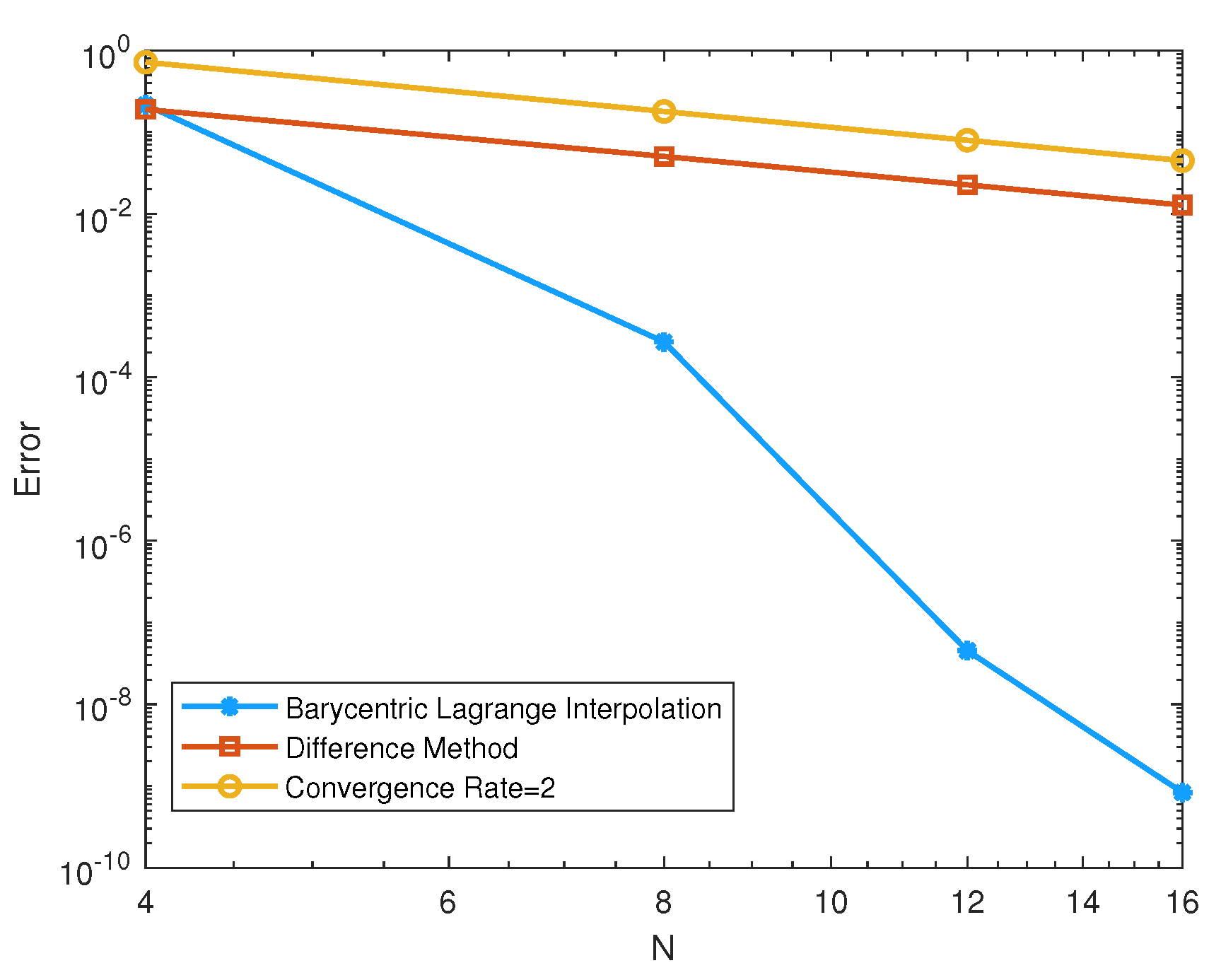
If we fix and vary the temporal step, , we can obtain errors and temporal convergence rate, as shown in Table 2. It shows that the MI scheme based on the barycentric interpolation collocation scheme for the NLS equation has second-order accuracy in time. In addition, the spatial convergence rate is also obtained, and the errors at time T = 1 for NLS equation are shown in Figure 1.
5.2. Example 2
Consider the following 1D problem on :
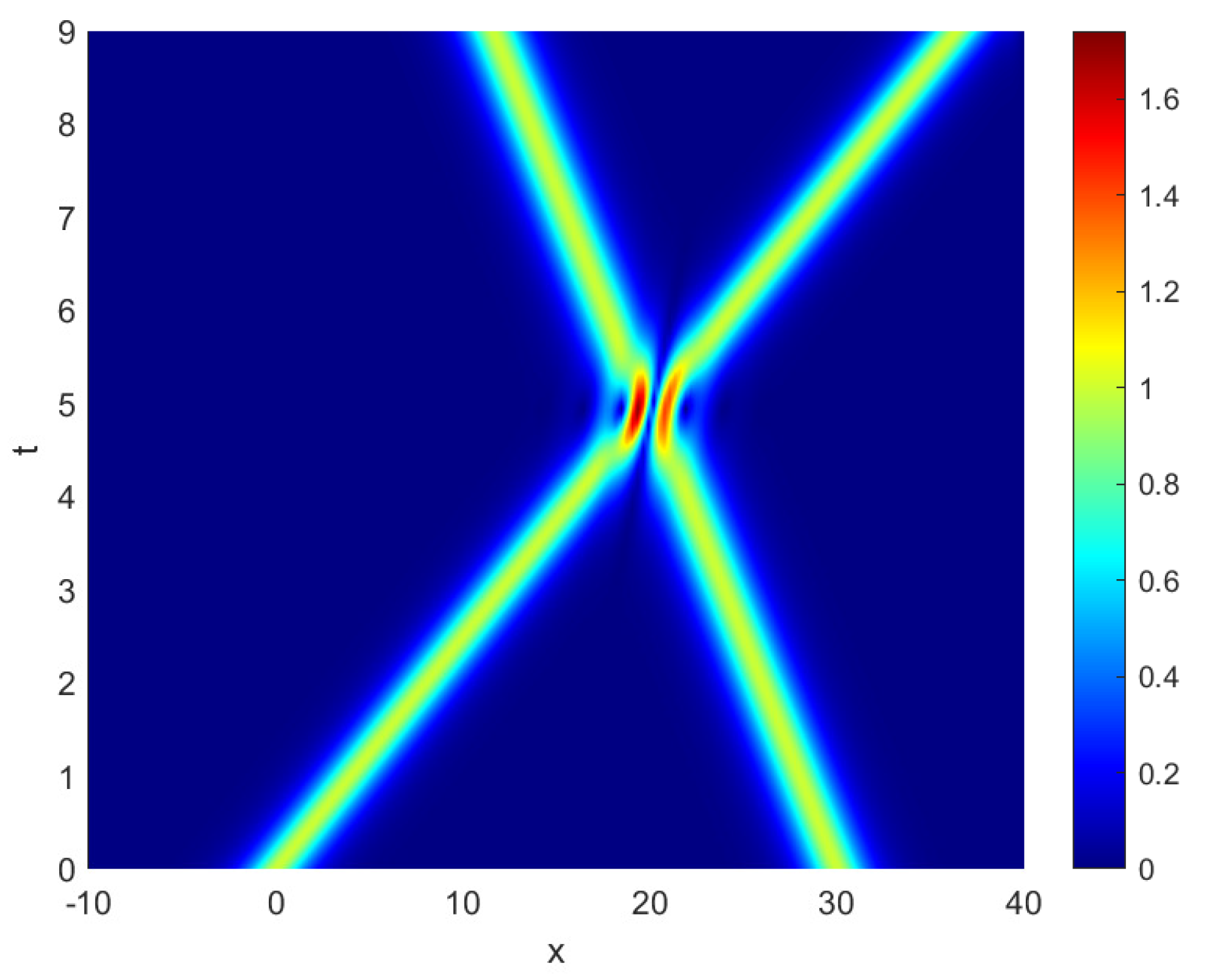
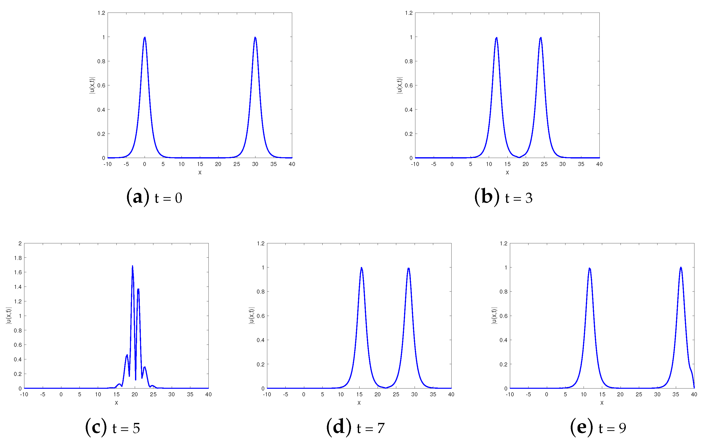
This example shows the collision behavior of two solitary waves. If we provide the initial value condition, a double solitary wave can be generated. When t = 0, two solitary waves are separated. The fast wave will catch up with the slow wave over time, and it will then surpass the slow wave after the collision, and there is only one phase change between them. This is consistent with the theory of waves; see Figure 4 and Figure 5.
6. Conclusions
In this work, we have proposed an effective operator splitting scheme based on the barycentric Lagrange interpolation collocation method for the nonlinear Schrödinger equation. The convergence analysis is proved theoretically and verified numerically. Numerical examples are presented to show the mass and energy conservation of the proposed scheme. The operator splitting collocation scheme is second-order in time and convergent exponentially in space. The two barycentric interpolation collocation schemes have high accuracy, and the barycentric Lagrange interpolation collocation method is slightly more efficient than the barycentric rational interpolation collocation method. Compared with the finite difference method, the barycentric interpolation collocation method can achieve high accuracy with fewer points. In the future, we plan to extend this method to coupled Schrödinger equations, KdV equations and Klein–Gordon equations, etc.
Author Contributions
M.Y., methodology, conceptualization, design, analysis, software, original draft writing; Z.W., methodology, supervision, conceptualization, editing, draft editing and reviewing. All authors have read and agreed to the published version of the manuscript.
Funding
The research was funded by the Natural Science Foundation of Fujian Province (Nos. 2022J01308, 2021J01306), the NSF of China (No. 11701197), the Program for Innovative Research Teams in Science and Technology in Fujian Province University and the Fuzhou-Xiamen-Quanzhou National Independent Innovation Demonstration Zone Collaborative Innovation Platform under Grant 2022FX5.
Data Availability Statement
No new data were created or analyzed in this study.
Acknowledgments
We thank the anonymous referees for their careful checking and valuable comments which improve the manuscript.
Conflicts of Interest
The authors declare no conflicts of interest.
References
- Schrödinger, E. The present status of quantum mechanics. Sci. Nat. 1935, 23, 1–26. [Google Scholar]
- Gong, Y.Z.; Wang, Q.; Wang, Y.S.; Cai, J.X. A conservative Fourier pseudo-spectral method for the nonlinear Schrödinger equation. J. Comput. Phys. 2017, 328, 354–370. [Google Scholar] [CrossRef]
- Cui, J.; Xu, Z.Z.; Wang, Y.S.; Jiang, C.L. Mass-and energy-preserving exponential Runge–Kutta methods for the nonlinear Schrödinger equation. Appl. Math. Lett. 2020, 112, 106770. [Google Scholar] [CrossRef]
- Feng, X.B.; Li, B.Y.; Ma, S. High-order mass-and energy-conserving SAV-Gauss collocation finite element methods for the nonlinear Schrödinger equation. SIAM J. Numer. Anal. 2021, 59, 1566–1591. [Google Scholar] [CrossRef]
- Wang, J.J.; Li, M.; Guo, L.J. Superconvergence analysis for nonlinear Schrödinger equation with two-grid finite element method. Appl. Math. Lett. 2021, 122, 107553. [Google Scholar] [CrossRef]
- Wang, L.L.; Li, M. Galerkin finite element method for damped nonlinear Schrödinger equation. Appl. Numer. Math. 2022, 178, 216–247. [Google Scholar] [CrossRef]
- Hu, H.Z.; Li, B.Y.; Zou, J. Optimal convergence of the Newton iterative Crank–Nicolson finite element method for the nonlinear Schrödinger equation. Comput. Methods Appl. Math. 2022, 22, 91–612. [Google Scholar] [CrossRef]
- Chen, C.J.; Lou, Y.Z.; Hu, H.Z. Two-grid finite volume element method for the time-dependent Schrödinger equation. Comput. Math. Appl. 2022, 108, 185–195. [Google Scholar] [CrossRef]
- Deng, B.C.; Shen, J.; Zhuang, Q.Q. Second-order SAV schemes for the nonlinear Schrödinger equation and their error analysis. J. Sci. Comput. 2021, 69, 88. [Google Scholar] [CrossRef]
- Su, C.M.; Zhao, X.F. On time-splitting methods for nonlinear Schrödinger equation with highly oscillatory potential. Math. Model. Numer. Anal. 2020, 54, 1491–1508. [Google Scholar] [CrossRef]
- Wang, T.C.; Zhao, X.F. Optimal L∞ error estimates of finite difference methods for the coupled Gross–Pitaevskii equations in high dimensions. Sci. China Math. 2014, 57, 2189–2214. [Google Scholar] [CrossRef]
- Li, J.; Qu, J.Z. Barycentric Lagrange interpolation collocation method for solving the Sine-Gordon equation. Wave Motion 2023, 120, 103159. [Google Scholar] [CrossRef]
- Hu, Y.D.; Peng, A.; Chen, L.Q.; Tong, Y.L.; Weng, Z.F. Analysis of the barycentric interpolation collocation scheme for the Burgers equation. Sci. Asia 2021, 47, 758–765. [Google Scholar] [CrossRef]
- Oruç, Ö. Two meshless methods based on local radial basis function and barycentric rational interpolation for solving 2D viscoelastic wave equation. Comput. Appl. Math. 2020, 79, 3272–3288. [Google Scholar] [CrossRef]
- Deng, Y.F.; Weng, Z.F. Barycentric interpolation collocation method based on Crank–Nicolson scheme for the Allen–Cahn equation. AIMS Math. 2021, 6, 3857–3873. [Google Scholar] [CrossRef]
- Deng, Y.F.; Weng, Z.F. Operator splitting scheme based on barycentric Lagrange interpolation collocation method for the Allen–Cahn equation. J. Appl. Math. Comput. 2022, 68, 3347–3365. [Google Scholar] [CrossRef]
- Huang, R.; Weng, Z.F. A numerical method based on barycentric interpolation collocation for nonlinear convection-diffusion optimal control problems. Netw. Heterog. Media 2023, 18, 562–580. [Google Scholar] [CrossRef]
- Yi, S.C.; Yao, L.Q. A steady barycentric Lagrange interpolation method for the 2D higher-order time-fractional telegraph equation with nonlocal boundary condition with error analysis. Numer. Methods Partial Differ. Equ. 2019, 35, 1694–1716. [Google Scholar] [CrossRef]
- Lubich, C. On splitting methods for Schrödinger–Poisson and cubic nonlinear Schrödinger equations. Math. Comput. 2008, 77, 2141–2153. [Google Scholar] [CrossRef]
- Zhai, S.Y.; Wang, D.L.; Weng, Z.F.; Zhao, X. Error analysis and numerical simulations of Strang splitting method for space fractional nonlinear Schrödinger equation. J. Sci. Comput. 2019, 81, 965–989. [Google Scholar] [CrossRef]
- Zhai, S.; Weng, Z.; Zhuang, Q.; Liu, F.; Anh, V. An effective operator splitting method based on spectral deferred correction for the fractional Gray–Scott model. J. Comput. Appl. Math. 2023, 425, 114959. [Google Scholar] [CrossRef]
- Berrut, J.P.; Trefethen, L.N. Barycentric Lagrange interpolation. SIAM Rev. 2004, 46, 501–507. [Google Scholar] [CrossRef]
- Strang, G. On the construction and comparison of difference schemes. SIAM J. Numer. Anal. 1968, 5, 506–517. [Google Scholar] [CrossRef]
- Li, J.; Cheng, Y.L. Linear barycentric rational collocation method for solving heat conduction equation. Numer. Methods Partial Differ. Equ. 2021, 37, 533–545. [Google Scholar] [CrossRef]
Figure 1.
Spatial errors at t = 1 for NLS equation for Example 1.

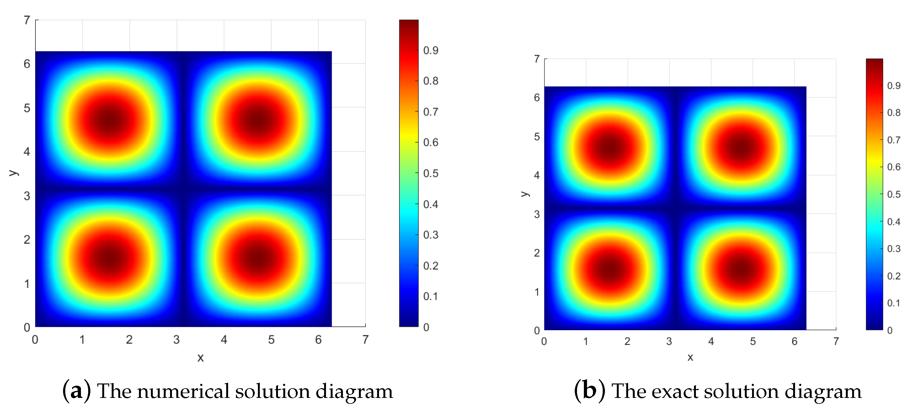
Figure 2.
The numerical solution and the exact solution diagrams at T = 1 for Example 1.

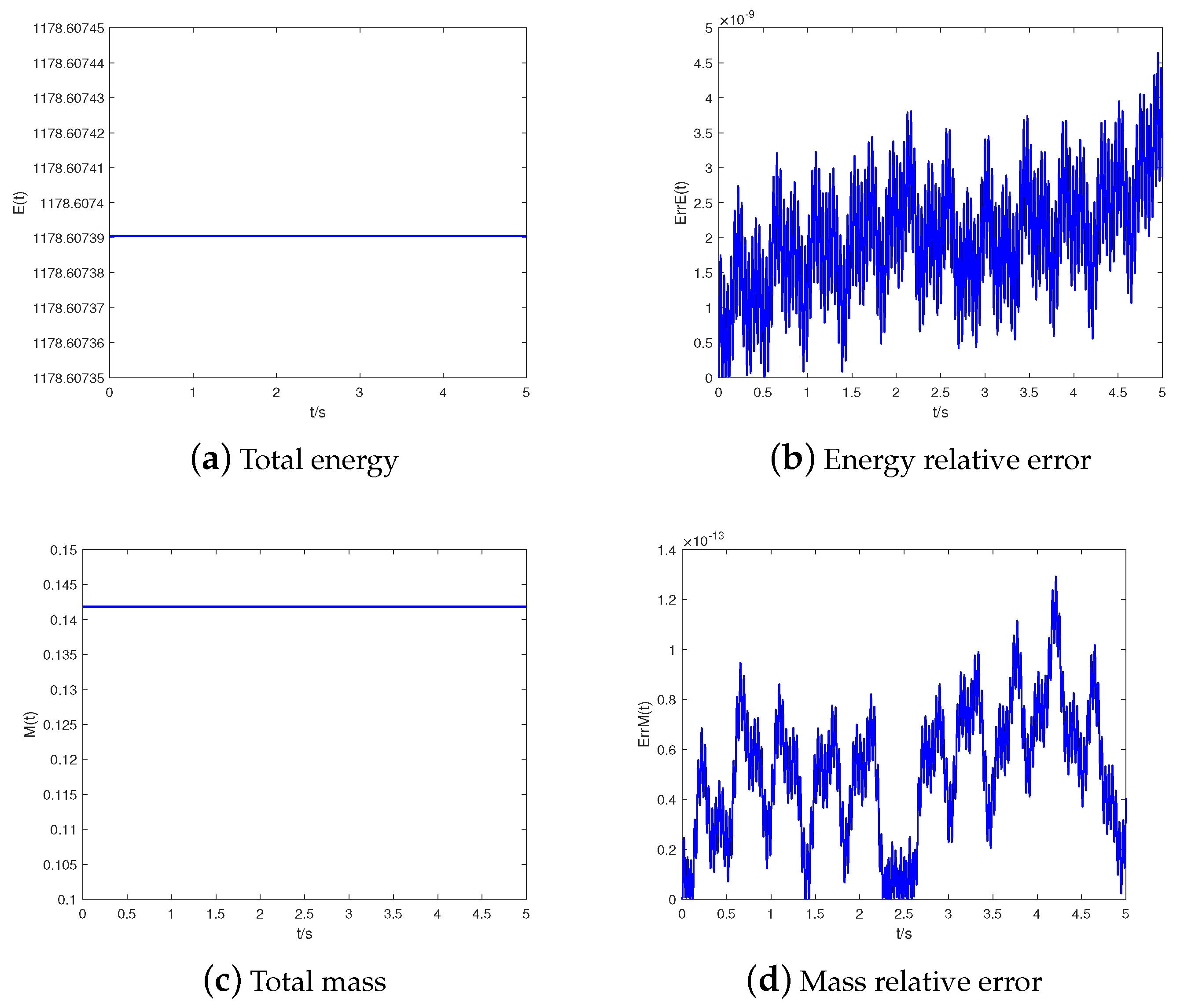
Figure 3.
Conservation situation of energy and mass at T = 1 for Example 1.

Figure 4.
The interaction of two solitary waves without damping at T = 9 for Example 2.

Figure 5.
Head-on collisions of two solitary waves without damping for Example 2.


Table 1.
Error of barycentric Lagrange interpolation collocation scheme for Example 1.
| m | |||
|---|---|---|---|
| 6 | 8.4010 × 10 | 8.4010 × 10 | 0.152 s |
| 8 | 2.3542 × 10 | 2.7054 × 10 | 0.288 s |
| 10 | 1.9318 × 10 | 2.0865 × 10 | 0.694 s |
| 12 | 5.6755 × 10 | 5.6755 × 10 | 1.039 s |
| 16 | 8.0816 × 10 | 8.3330 × 10 | 2.914 s |
Table 2.
Error of barycentric rational interpolation collocation method for Example 1.
| m | |||
|---|---|---|---|
| 6 | 2.9302 × 10 | 2.9302 × 10 | 0.178 s |
| 8 | 2.7122 × 10 | 3.1167 × 10 | 0.289 s |
| 10 | 5.4257 × 10 | 5.8602 × 10 | 0.735 s |
| 12 | 2.0948 × 10 | 2.0948 × 10 | 1.082 s |
| 16 | 8.3994 × 10 | 8.6607 × 10 | 3.066 s |
Table 3.
Error of difference scheme for Example 1.
| m | |||
|---|---|---|---|
| 10 | 2.9367 × 10 | 3.2467 × 10 | 0.202 s |
| 20 | 8.1977 × 10 | 8.1977 × 10 | 3.586 s |
| 40 | 2.0546 × 10 | 2.0546 × 10 | 160.534 s |
| 60 | 9.1360 × 10 | 9.1360 × 10 | 1665.769 s |
| 80 | 5.1402 × 10 | 5.1402 × 10 | 8993.522 s |
Table 4.
Errors and convergence rate in time for Example 1.
| 1/8 | 1.2598 × 10 | - | 1.2990 × 10 | - |
| 1/16 | 3.1552 × 10 | 1.9975 | 3.2533 × 10 | 1.9975 |
| 1/32 | 7.8913 × 10 | 1.9994 | 8.1368 × 10 | 1.9994 |
| 1/64 | 1.9731 × 10 | 1.9998 | 2.0344 × 10 | 1.9998 |
Disclaimer/Publisher’s Note: The statements, opinions and data contained in all publications are solely those of the individual author(s) and contributor(s) and not of MDPI and/or the editor(s). MDPI and/or the editor(s) disclaim responsibility for any injury to people or property resulting from any ideas, methods, instructions or products referred to in the content. |
© 2024 by the authors. Licensee MDPI, Basel, Switzerland. This article is an open access article distributed under the terms and conditions of the Creative Commons Attribution (CC BY) license (https://creativecommons.org/licenses/by/4.0/).
Share and Cite
MDPI and ACS Style
Yao, M.; Weng, Z. A Numerical Method Based on Operator Splitting Collocation Scheme for Nonlinear Schrödinger Equation. Math. Comput. Appl. 2024, 29, 6. https://doi.org/10.3390/mca29010006
AMA Style
Yao M, Weng Z. A Numerical Method Based on Operator Splitting Collocation Scheme for Nonlinear Schrödinger Equation. Mathematical and Computational Applications. 2024; 29(1):6. https://doi.org/10.3390/mca29010006
Chicago/Turabian StyleYao, Mengli, and Zhifeng Weng. 2024. "A Numerical Method Based on Operator Splitting Collocation Scheme for Nonlinear Schrödinger Equation" Mathematical and Computational Applications 29, no. 1: 6. https://doi.org/10.3390/mca29010006