Spatially Resolved, Real-Time Polarization Measurement Using Artificial Birefringent Metallic Elements


Applied Laser and Photonics Group, Faculty of Engineering, Aschaffenburg Technical University of Applied Sciences, Wuerzburger Str. 45, 63743 Aschaffenburg, Germany
*
Author to whom correspondence should be addressed.
Photonics 2024, 11(5), 397; https://doi.org/10.3390/photonics11050397
Submission received: 25 March 2024
/
Revised: 19 April 2024
/
Accepted: 23 April 2024
/
Published: 24 April 2024
(This article belongs to the Special Issue Polarization Optics)
Abstract
:Polarization states define a fundamental property in optics. Consequently, polarization state characterization is essential in many areas of both field industrial applications and scientific research. However, a full identification of space-variant Stokes parameters faces great challenges, like multiple power measurements. In this contribution, we present a spatially resolved polarization measurement using artificial birefringent metallic elements, the so-called hollow waveguides. Differently oriented and space-variant hollow waveguide arrays, a stationary analyzer and a CMOS camera form the basis of the experimental setup for one single spatially resolved power measurement. From this power measurement, the Stokes parameters can be calculated in quasi-real-time, with a spatial resolution down to 50 μm in square. The dimensions of the individual hollow waveguides, which are less than or equal to the employed wavelength, determine the spectral range, here in the near infrared around = 1550 nm. This method allows for the rapid and compact determination of spatially resolved Stokes parameters, which is experimentally confirmed using defined wave plates, as well as an undefined injection-molded polymer substrate.
1. Introduction
Light, as an electromagnetic wave, exhibits several fundamental properties, such as the scalar quantities intensity and frequency, as well as polarization as a vectorfield quantity [1,2]. The state of polarization—the orientation of the accompanying electric vector—is essential in various fields, including industrial applications, everyday life and scientific research. In industrial applications, for instance in laser material processing, the state of polarization influences the absorption behavior of the material [3,4]. Polarization in everyday life can be observed, e.g., in the use of LCD screens or when visiting a 3D cinema [5,6]. In scientific research, there are diverse application areas significantly influenced by polarization, such as polarization imaging for clinical and biological applications [7,8,9]. While scalar quantities are relatively straightforward to determine, measuring polarization requires increased time and instrumental effort [10]. Determining the state of polarization is possible through multiple measurements of the same signal. The state of polarization can be described by the Stokes vector S, which consists of four individual Stokes parameters ( to ). Each necessary measurement serves to ascertain one of the vector components of S, the Stokes parameters ( to ) [11].
There are numerous techniques to determine the Stokes parameters. One of the most commonly used methods involves a rotating linear retarder followed by a fixed linear polarizer [12]. The signal transmitted through this setup is measured with a photodetector. The transmitted intensity depends on the angle of the rotating linear retarder. The individual Stokes parameters can be calculated from the measured intensity values. To avoid moving parts, the rotating linear retarder can be replaced by photo-elastic modulators [13], liquid crystals [14], or by Pockels cells [15]. Nevertheless, the mentioned measurement methods involve sequential measurements. To perform these measurements simultaneously, the signal to be measured is either divided into multiple beam paths (amplitude division), distributed over a series of analyzers (wavefront division), or measured multiple times with a time-variable analyzer (time division) [16,17]. Another challenge is to not average the state of polarization over the area of interest, but rather to depict the Stokes parameters in a spatially resolved manner. Various approaches are presented in the literature to address these challenges, including the use of aluminum nanowires [18], elliptical polarizers [19], or metastructures [20,21,22].
With this work, we aim to contribute to the spatially resolved measurement of the Stokes parameters. The approach for this work originates from Helfert et al. This group demonstrated, in a theoretical study, the possibility of spatially changing the polarization states using hollow waveguides, which are well-known in microwave technology [23]. A specific research question of this group is to improve the coupling of Terahertz waves to metallic wires [24]. The group initially demonstrated practical experiments using non-spatially resolved hollow waveguides in the visible spectrum [25]. Collaborating with this group, we have transferred and further developed the fabrication to 3D direct laser writing [26]. A specific application that motivates our work is the application of measuring the stress-induced birefringence in bulk polymers demonstrated in this article. The authors are engaged in integrating optical sensor elements into bulk polymers. Understanding stress-induced birefringence is crucial for selectively exciting modes and increasing the sensitivity of the sensors [27].
In this article, we have succeeded in developing a compact spatially resolved polarimeter capable of determining the Stokes parameter in quasi-real-time. Figure 1 serves as a graphical summary providing an overview of the present work. The core of the work is the space-variant polarimeter comprising a hollow waveguide array with four different arranged hollow waveguide regions and a fixed linear polarizer. In conjunction with a CMOS camera, it is possible to perform intensity measurements with spatial resolution through the four different arranged hollow waveguide regions, which are necessary for calculating the Stokes parameters of any polarisation state.
In Figure 1, the four different regions of the hollow waveguide array are schematically depicted in orange, blue, gray and yellow. Just for completeness, it should be mentioned that the hollow waveguide array consists of numerous such regions, known as polarization pixels. Moreover, individual regions consist of more than just one hollow waveguide, as depicted here in a simplified manner. Figure 1 also depicts in the upper part the polarization states before the sample to be measured (PS1), after the sample (PS2), and after the spatial variant polarimeter (PS3). The input polarization state is set as being linearly horizontal polarized by the polarization direction of the laser and a linear polarizer. This is a fixed polarization state, and is not changed during the measurements. Through the sample to be measured, the polarization state changes after the sample depending on the polarization sensitive optical properties of the sample. The spatial variant polarimeter then categorizes the different polarization states into linearly horizontal, linearly vertical, linearly polarized light at an angle of 45°, and circularly polarized light. With the subsequent CMOS camera, the incident intensity values of the four regions are measured and, from this, the Stokes parameters are determined. With this setup, it is possible to measure all types of polarization states.
The advantages of this approach, compared to other methods like rotating quarter wave plates, for measuring the Stokes parameters lies in its spatially compact design; all components of the setup are permanently installed, are not movable, and do not need to be moved [28,29]. Spatially large elements can be fabricated; the order of magnitude of a hollow waveguide array can be in the range of several centimeters, a scale that, for example, is only achievable with a high temporal manufacturing effort with metastructures [30,31].
One disadvantage of this method is that it is always spectrally limited to a single wavelength. For example, metastructures have an advantage here, as they can be partially utilized for a broader spectral range [32]. Another drawback is observed in the size of the waveguides; beyond a certain size, they cannot be further reduced with the chosen manufacturing method. For further size reduction, a switch to a different manufacturing method would be necessary, such as electron beam lithography [33].
Beyond the applications shown later in this work, the use of this spatially resolved polarimeter can be seen in material analysis and laser material processing. The layout of the hollow waveguides can be tailored to specific needs and easily integrated into an optical setup. This allows for applications such as spatially resolved polarimetry, as well as the generation of the spatially resolved polarization states required in laser material processing. To cover an even wider range of applications, a focus of further work is to reduce the size of the hollow waveguides to adapt the spatially resolving polarimeter for wavelengths in the visible range.
2. Design
Hollow waveguides are structures that induce an artificial birefringence through their geometry. Given a waveguide height h and an operating wavelength , the effective refractive index of propagating modes depends solely on the waveguide apertures , and can be calculated by Equation (1):
The desired phase shift is directly related to the effective refractive index , and can be calculated by Equation (2):
where . In the context of this study, the dimensions of the hollow waveguides are defined accordingly, such that only the two fundamental modes TE1,0 and TE0,1 are propagating. The dimension for the waveguide opening is identical for all hollow waveguides, and is set to = 1550 nm. The waveguide opening is adjusted according to the required phase shift, with = 872 nm for a half-wave plate and = 1034 nm for a quarter-wave plate. The entire hollow waveguide array has a uniform height of h = 1.9 µm.
The design of the spatially variant polarimeter does not include any moving parts. It consists solely of an inhomogeneous hollow waveguide array, a fixed analyzer, and a CMOS camera to detect the light intensity. To calculate the Stokes parameters, four different intensity measurements need to be conducted, and these are carried out simultaneously. To enable this, the hollow waveguides are arranged into a so-called polarization pixel. Each of these polarization pixels consists of four subpixels. Figure 2 shows a polarization pixel (enclosed in dotted lines) consisting of four subpixels labeled from I to IV. Additionally, each subpixel is marked with a different color (orange, blue, gray, and yellow). Three subpixels consists of half-wave plates with different orientations, while the fourth subpixel is a quarter-wave plate. The transmission axis of the analyzer in the optical setup is set at a fixed angle of = 45°, and is not changed during the measurements. The hollow waveguide array is also fixed within the setup.
The four intensity values required to calculate the Stokes parameters are determined spatially variant per polarization pixel through the different orientations and phase delays of the four subpixles. The Stokes parameter can be calculated from the spatially variant measured intensity values using Equations (3)–(6):
The design presented here enables the complete characterization of an input beam with unknown polarization in less than half of a second for a specific wavelength, here = 1550 nm. To measure the Stokes parameters for another specific wavelength, the lateral dimensions or the height h of the hollow waveguides must be adjusted according to Equations (1) and (2). From a technological perspective, the fabrication of hollow waveguides for a wavelength of 600 nm is feasible. For measuring the Stokes parameters for different wavelengths, the hollow waveguide arrays can be easily exchanged, comparable, for example, to bandpass filters in a fluorescence microscope. To perform a true spatially resolved polarization measurement, it is necessary to miniaturize the four subpixels. A polarization pixel has a side length of 100 μm in both x and y directions, and a single subpixel has a length of 50 μm in both x and y directions. Such a side length is well achievable with the chosen manufacturing process, consisting of a two-stage fabrication using 3D direct laser writing and micro-electrodeposition. From a manufacturing perspective, a minimal side length of a complete polarization pixel of 20 μm is conceivable. By repetitively arranging the polarization pixels in the x and y directions, it is possible to manufacture a spatially variant polarimeter with a complete size in the centimeter range. The sensitivity of the polarimeter is directly dependent on the bit depth of the CMOS camera. The greater the bit depth, the higher the sensitivity. Table 1 presents all of the conditions required for measuring the intensities and calculating the Stokes parameters.
3. Materials and Methods
3.1. Fabrication of the Hollow Waveguide Array
The fabrication of the spatially variant polarimeter involves a two-stage manufacturing process. First, a negative of the final hollow waveguide array is fabricated using 3D direct laser writing (3D DLW, Nanoscribe GmbH & Co. KG (Eggenstein-Leopoldshafen, Germany), Type Photonic Professional GT2). This involves exposing a positive photoresist (MicroChemicals GmbH (Ulm, Germany), Type AZ 3027) using 3D DLW. Following to exposure and subsequent development, free-standing photoresist pillars are formed on the indium tin oxide (ITO)-coated glass substrate, separated by trenches with a width of 300 nm. In the second stage of fabrication, the trenches are filled with gold using a micro-electrodeposition process (Potentiostat: AMETEK GmbH (Meerbusch, Germany), Type VersaSTAT 4; Hotplate: Carl Roth GmbH & Co. KG (Karlsruhe, Germany), Type MH 20). Due to poor adhesion of gold to an ITO surface, the hollow waveguide array is fixed onto the substrate through a standard lithography step. During the development process of the standard lithography step, the photoresist pillars still present in the gold-coated structure of the hollow waveguides are removed.
A detailed fabrication of the hollow waveguide array is provided by the authors in Ref. [34]. To facilitate a thorough understanding of the fabrication process, reference is made to this publication. The spatially variant polarimeter fabricated here differs from the production described in [34] in one aspect: the hollow waveguides are not horizontally arranged, but are tilted at various angles relative to the horizontal plane. The corresponding angles and related dimensions of the waveguides are presented in Table 1. Figure 3 shows an overview of the fabricated structure (Figure 3, left), as well as a detailed view of the respective subpixels I–IV (Figure 3, right).
3.2. Experimental Setup
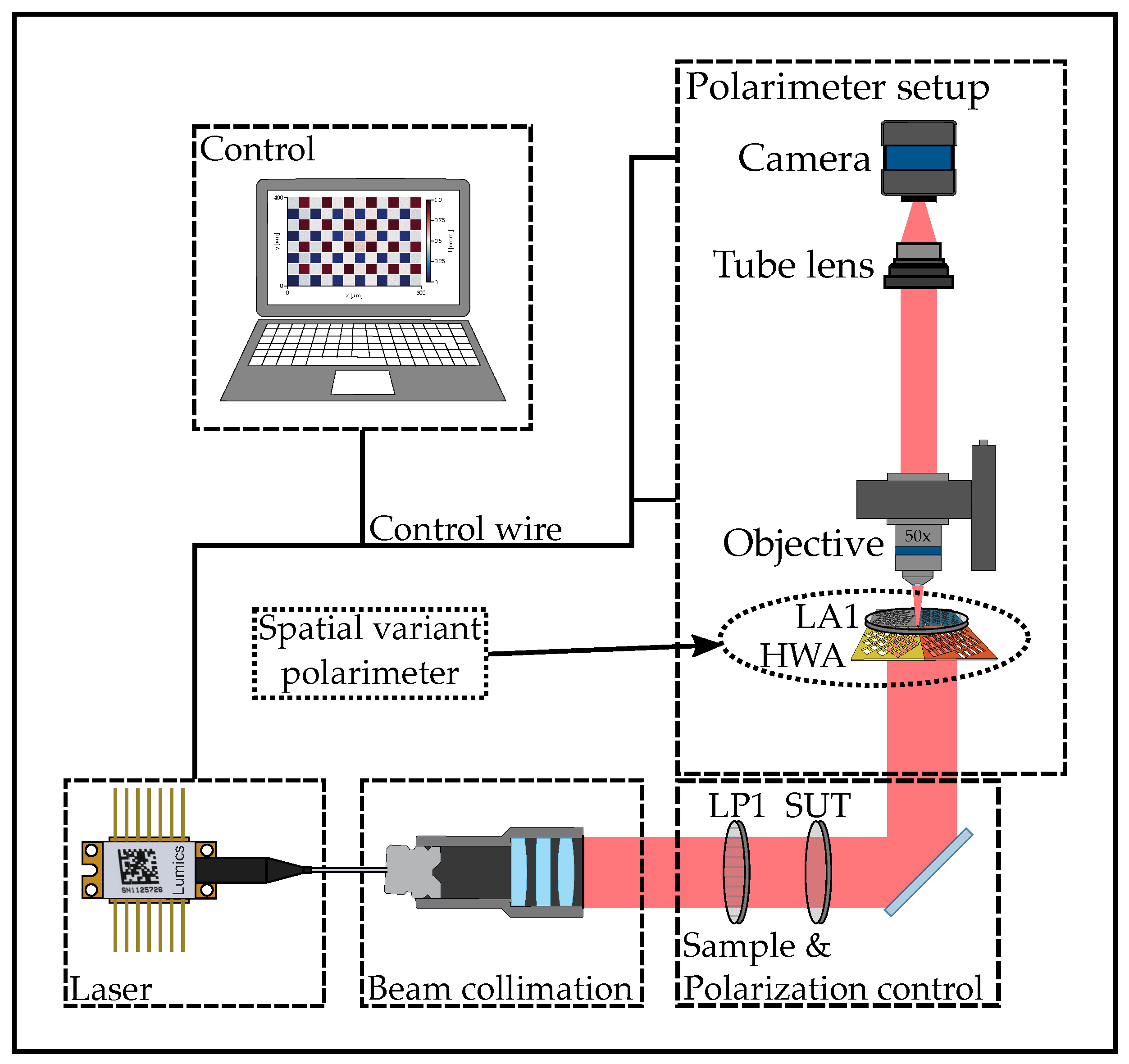
The linearly polarized radiation, = 1550 nm, of a fiber-coupled laser diode (Lumics GmbH (Berlin, Germany), Type LU1550M150-1A06F30H) is collimated to a beam diameter of 1.1 mm by means of a collimation unit (Thorlabs GmbH (Bergkirchen, Germany), Type TC06FC-1550). Following to the beam collimation, there is a linear polarizer (LP1), which sets the polarization direction of the beam to linear horizontal polarization. Immediately after the linear polarizer, the sample under test (SUT) is installed. Subsequently, the spatially resolved polarimeter is positioned for the evaluation of the Stokes parameters. This consists of the hollow waveguide array (HWA) described in the previous subsection and a fixed analyzer (LA1). The latter exhibits a rotation angle of 45° with respect to horizontal plane. The output after the HWA and the analyzer is imaged onto a CMOS camera (Edmund Optics GmbH (Mainz, Germany), Type 1460–1600 nm Near-Infrared Camera) using 50× objective (Mitutoyo GmbH (Neuss, Germany), Type M Plan Apo NIR HR 50×) and a tube lens (Thorlabs GmbH (Bergkirchen, Germany), Type TTL200-S8). Figure 4 illustrates the measurement setup in a schematic drawing.
3.3. Evaluation Algorithm
For the evaluation and graphical representation of the Stokes parameters, the intensity distribution detected by the CMOS camera must be normalized and rearranged. For an accurate calculation of the Stokes parameters, it is necessary to incorporate a correction factor for the /4 sub-pixels. This consideration is essential, because the larger area due to > leads to a relatively higher transmitted intensity, making the individual sub-pixels incomparable. To estimate a correction factor, the area of the hollow waveguides in sub-pixels II and IV is determined based on images obtained with a scanning electron microscope, resulting in a 1.18 times larger /4 sub-pixel compared to the /2 sub-pixel. For normalization, the intensity of sub-pixel IV is divided by the correction factor and, finally, all camera pixels are divided by the maximum pixel value. Figure 5 shows the intensity distribution of the camera image after normalization. This figure exemplifies the normalized intensity distribution of the linear horizontally polarized input radiation (top image).
The mean intensity values are calculated from the individual sub-pixels. Using these mean values and applying Equations (3)–(6), the Stokes parameters to are calculated from the individual polarization pixels. Optimization of the achievable spatial resolution is achieved by using an overlapping pixel arrangement, as depicted in Figure 5(bottom). The first polarization pixel (orange-dashed) represents the individual intensities for calculating the Stokes parameter in the orange region (0; 0). The second polarization pixel (blue-dashed) consists half of the first polarization pixel and half of the polarization pixel adjacent in the x-direction. It overlaps with the first polarization pixel and forms the basis for calculating the Stokes parameters in the blue field (1; 0). This procedure of overlapping polarization pixels is continued row by row and column by column, resulting in a spatially resolved representation of 50 μm for the Stokes parameters. The spatial resolution of the polarimeter, with a fixed magnification of the imaging optics, is directly dependent on the edge length of the individual sub-pixels, and can be further reduced by manufacturing techniques. As described in previous paragraphs, the Stokes parameters can be displayed in quasi-real-time. From reading the camera image to the computation time for evaluation to the presentation of the measurement results, 0.463 s elapses.
4. Results and Discussion
To verify its functionality, the space-variant polarimeter is characterized using a quarter- and a half-wave plate. The samples to be characterized are installed after beam collimation and before entering the spatial variant polarimeter. For characterization, the retardation plates are rotated in 7.5° steps from −45° to 45° for the quarter-wave plate and from 0° to 90° for the half-wave plate.
Figure 6 shows the spatially resolved Stokes parameters as a function of the orientation angle of a quarter-wave plate. The upper three rows represent the calculated spatially resolved Stokes parameters, with each Stokes parameter to per column and with different orientations of the quarter-wave plate per row. In the bottom row, three plots depict the Stokes parameters to . The measured values are marked with unfilled circles. Furthermore, the three filled circles represent the measured values depicted in the top upper three rows. In addition to the measured values, the theoretical curve of the Stokes parameters of a quarter-wave plate is plotted. The Stokes parameters depicted in the top row indicate a circular polarization state oriented counterclockwise. This occurs when linear horizontally polarized incident light passes through a quarter-wave plate with maximum phase delay. The middle row shows the Stokes parameters for an angle position of = −15° of the quarter-wave plate. The maximum phase delay between the two propagating modes decreases, and the state of polarization approaches that of the incident radiation. Consequently, the linear components of polarization at the output increase while the circular component decreases. This results in elliptical polarization oriented counterclockwise. Changing the angle position from = −15° to = 15° yields approximately the same magnitudes compared to the previous angle position, but with a small difference. The elliptical polarization changes its rotation direction from counterclockwise to clockwise. There are only slight differences between the Stokes parameters of the angle position −15° and 15°, which can be attributed to a slightly incorrect angle position. For all of the angle position of the quarter-wave plate, the measured Stokes parameters closely match the theoretical curve. The further measured values also exhibit only slight deviations within the measurement range. Overall, all measured values show very good agreement between the actual measured and theoretical trajectories of the Stokes parameters.
Figure 7 shows the spatially resolved Stokes parameters for various angle positions of a half-wave plate. In contrast to a quarter-wave plate, a half-wave plate does not change the polarization state from linear to circular, it maintains a linearly polarized output radiation over the entire angular range. The absence of a circular component corresponds to a value of zero for the Stokes parameter , which is clearly visible in the images and in the corresponding diagram of Figure 7. In the first row of Figure 7, the half-wave plate is in its initial state at = 0°, meaning the linear horizontal input polarization lies exactly along the fast axis of the half-wave plate. The propagating modes experience no phase delay, and the polarization state of the light after the half-wave plate matches the input polarization state. The angle position of the half-wave plate for the measurements in the middle row is = 30°. Due to the change in angle, the fast axis rotates, and the propagating modes experience a phase delay. The direction of polarization changes from linear horizontally polarized to linearly polarized state at an angle. Further rotation of the half-wave plate to an angle of = 45° results in a change in the direction of polarization to linear vertically polarized light. Similar to the measurements of the quarter-wave plate, all values measured here are in excellent agreement, and show only slight deviations from the theoretical trajectory.
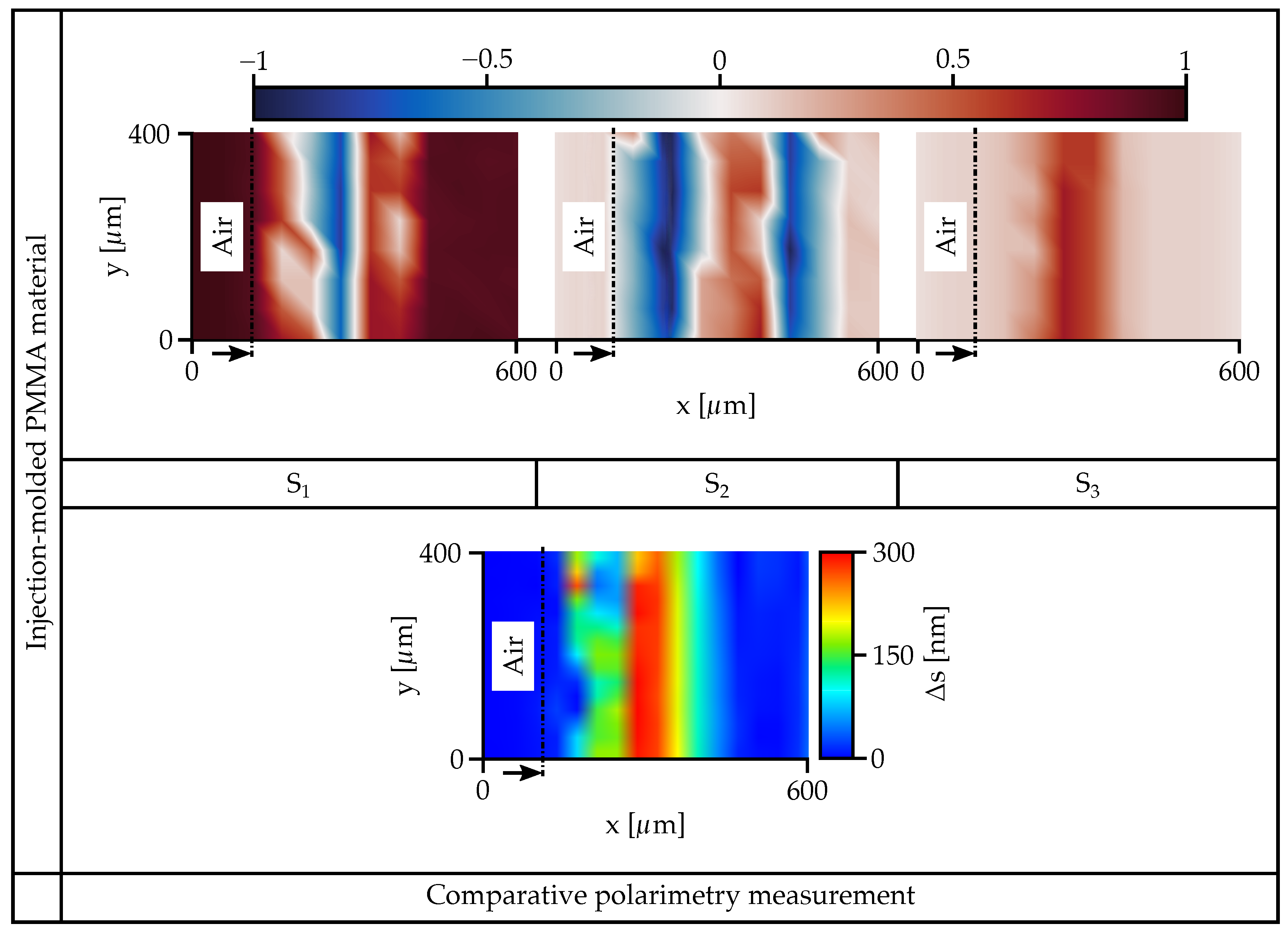
In the measurements with known phase delays, the functionality of the spatially variant polarimeter could be well demonstrated. As a sample with an unknown spatially variant phase delay, the edge of a 1.3 mm thick polymethylmethacrylate plate (Goodfellow GmbH (Hamburg, Germany), Type ME303018) is examined. The plate is a commercially available product manufactured by injection molding. In the relaxed state, polymers exhibit isotropic material properties. Due to the high pressure during the injection molding process, tensile and shear forces occur in the material, leading to alignment of the polymer chains. This alignment is more pronounced at the material surfaces, as there is a faster cooling of the material. The alignment of the polymer chains results in optical anisotropy [35].
A promising application for the use of injection-molded polymer substrates are integrated photonic elements such as waveguides and optical sensors [36,37]. The optical anisotropy introduced by cooling causes birefringent behavior of the photonic structures, and has influence on the mechanical properties of the substrates. For example, various investigations have shown that the transmission behavior of waveguides is strongly dependent on the polymer orientation. The sensor signals from Bragg gratings written into waveguides are also direction-dependent [38]. Understanding optical anisotropy in injection-molded polmyer substrates can significantly impact the functionality of integrated optical elements.
The measurement results in Figure 8 show that spatially variant measurement of the Stokes parameters is also feasible for a sample with an unknown phase delay. In the outer edge region of the sample, from the sample surface (x = 100 µm) to x = 350 µm a change in the Stokes parameters can be measured. Beyond x = 350 µm, the optical anisotropy decreases. The high optical anisotropy of the material can arise from flow conditions or uneven cooling during injection molding. Flow-induced alignment of the molecule chains occurs along the flow direction, and they solidify at different rates due to uneven cooling. The formation of anisotropic regions during cooling is also known from the literature, and is described, for example, in Refs. [39,40]. A comparative measurement of the same sample is shown in the lower part of Figure 8 using a commercially available polarimeter (Ilis GmbH (Germany, Erlangen), Type StrainScope Flex). Both spatially resolved measurements demonstrate the optically anisotropic behavior at the edge of the sample very well, and are highly comparable.
5. Conclusions
In this contribution, we have investigated the application possibilities of hollow waveguides as a spatially resolved polarimeter. We have demonstrated that the polarimeter enables simultaneous spatially resolved measurement of the Stokes parameters in quasi-real-time, with = 0.463 s. To achieve simultaneous measurement of the Stokes parameters, the dimensions and orientation of the hollow waveguides are divided into so-called polarization pixels, each with a width of 100 in square. Coupled with a fixed linear polarization analyzer and a CMOS camera, spatially resolved measurement is possible. The functionality of the spatially resolved polarimeter was demonstrated using elements with defined phase delay (quarter- and half-wave plates) for a wavelength of = 1550 nm of the optical radiation. To test its application on a sample with unknown phase delay, the edge region of an injection-molded polymethylmethacrylate plate was examined. The results obtained were comparable to those acquired with a polarimeter for industrial purposes. The approach presented in the article demonstrates the feasibility of constructing a spatially resolved polarimeter using hollow waveguides. The setup does not contain any moving components, and the readout speed is limited only by the processing speed of the image acquisition software (version number V3).
Author Contributions
Conceptualization, S.B. and R.H.; methodology, S.B.; software, S.B. and S.K.; validation, S.B., S.K. and R.H.; formal analysis, S.B.; investigation, S.B.; resources, R.H.; data curation, S.B. and S.K.; writing—original draft preparation, S.B., S.K. and R.H.; writing—review and editing, S.B., S.K. and R.H.; visualization, S.B.; supervision, R.H.; project administration, R.H. All authors have read and agreed to the published version of the manuscript.
Funding
This research received no external funding.
Institutional Review Board Statement
Not applicable.
Informed Consent Statement
Not applicable.
Data Availability Statement
Data underlying the results presented in this paper are not publicly available at this time but may be obtained from the authors upon reasonable request.
Conflicts of Interest
The authors declare no conflicts of interest.
References
- Huard, S. Polarization of Light; John Wiley and Sons Masson: Chichester, UK; New York, NY, USA; Paris, France, 1997. [Google Scholar]
- Goldstein, D.H. Polarized Light; CRC Press: Boca Raton, FL, USA, 2017. [Google Scholar] [CrossRef]
- Meier, M.; Romano, V.; Feurer, T. Material processing with pulsed radially and azimuthally polarized laser radiation. Appl. Phys. A 2007, 86, 329–334. [Google Scholar] [CrossRef]
- Patel, A.; Tikhonchuk, V.T.; Zhang, J.; Kazansky, P.G. Non-paraxial polarization spatio-temporal coupling in ultrafast laser material processing. Laser Photonics Rev. 2017, 11, 1600290. [Google Scholar] [CrossRef]
- Srivastava, A.K.; De Bougrenet De La Tocnaye, J.L.; Dupont, L. Liquid crystal active glasses for 3D cinema. J. Disp. Technol. 2010, 6, 522–530. [Google Scholar] [CrossRef]
- Richtberg, S.; Girwidz, R. Use of linear and circular polarization: The secret LCD screen and 3D cinema. Phys. Teach. 2017, 55, 406–408. [Google Scholar] [CrossRef]
- Oldenbourg, R. A new view on polarization microscopy. Nature 1996, 381, 811–812. [Google Scholar] [CrossRef] [PubMed]
- Ding, C.; Li, C.; Deng, F.; Simpson, G.J. Axially-offset differential interference contrast microscopy via polarization wavefront shaping. Opt. Express 2019, 27, 3837. [Google Scholar] [CrossRef]
- Morizet, J.; Ducourthial, G.; Supatto, W.; Boutillon, A.; Legouis, R.; Schanne-Klein, M.C.; Stringari, C.; Beaurepaire, E. High-speed polarization-resolved third-harmonic microscopy. Optica 2019, 6, 385. [Google Scholar] [CrossRef]
- Juhl, M.; Mendoza, C.; Mueller, J.P.B.; Capasso, F.; Leosson, K. Performance characteristics of 4-port in-plane and out-of-plane in-line metasurface polarimeters. Opt. Express 2017, 25, 28697. [Google Scholar] [CrossRef]
- Gu, N.; Yao, B.; Huang, L.; Rao, C. Design and analysis of a novel compact and simultaneous polarimeter for complete Stokes polarization imaging with a piece of encoded birefringent crystal and a micropolarizer array. IEEE Photonics J. 2018, 10, 1–12. [Google Scholar] [CrossRef]
- Sabatke, D.S.; Descour, M.R.; Dereniak, E.L.; Sweatt, W.C.; Kemme, S.A.; Phipps, G.S. Optimization of retardance for a complete Stokes polarimeter. Opt. Lett. 2000, 25, 802. [Google Scholar] [CrossRef]
- Guan, W.; Cook, P.J.; Jones, G.A.; Shen, T.H. Experimental determination of the Stokes parameters using a dual photoelastic modulator system. Appl. Opt. 2010, 49, 2644–2652. [Google Scholar] [CrossRef]
- Bueno, J.M. Polarimetry using liquid-crystal variable retarders: Theory and calibration. J. Opt. A Pure Appl. Opt. 2000, 2, 216–222. [Google Scholar] [CrossRef]
- Kaneshiro, J.; Watanabe, T.M.; Fujita, H.; Ichimura, T. Full control of polarization state with a pair of electro-optic modulators for polarization-resolved optical microscopy. Appl. Opt. 2016, 55, 1082. [Google Scholar] [CrossRef]
- Balthasar Mueller, J.P.; Leosson, K.; Capasso, F. Ultracompact metasurface in-line polarimeter. Optica 2016, 3, 42. [Google Scholar] [CrossRef]
- Peinado, A.; Lizana, A.; Campos, J. Design of polarimeters based on liquid crystals and biaxial crystals for polarization metrology. Opt. Pura Apl. 2016, 49, 167–177. [Google Scholar] [CrossRef]
- Gruev, V.; Perkins, R.; York, T. CCD polarization imaging sensor with aluminum nanowire optical filters. Opt. Express 2010, 18, 19087. [Google Scholar] [CrossRef]
- Hsu, W.L.; Myhre, G.; Balakrishnan, K.; Brock, N.; Ibn-Elhaj, M.; Pau, S. Full-Stokes imaging polarimeter using an array of elliptical polarizer. Opt. Express 2014, 22, 3063. [Google Scholar] [CrossRef]
- Arbabi, E.; Kamali, S.M.; Arbabi, A.; Faraon, A. Full-Stokes imaging polarimetry using dielectric metasurfaces. ACS Photonics 2018, 5, 3132–3140. [Google Scholar] [CrossRef]
- Intaravanne, Y.; Chen, X. Recent advances in optical metasurfaces for polarization detection and engineered polarization profiles. Nanophotonics 2020, 9, 1003–1014. [Google Scholar] [CrossRef]
- Huang, Z.; Zheng, Y.; Li, J.; Cheng, Y.; Wang, J.; Zhou, Z.K.; Chen, L. High-resolution metalens imaging polarimetry. Nano Lett. 2023, 23, 10991–10997. [Google Scholar] [CrossRef]
- Helfert, S.F.; Edelmann, A.; Jahns, J. Hollow waveguides as polarization converting elements: A theoretical study. J. Eur. Opt. Soc. Rapid Publ. 2015, 10, 15006. [Google Scholar] [CrossRef]
- Edelmann, A.; Moeller, L.; Jahns, J. Coupling of terahertz radiation to metallic wire using end-fire technique. Electron. Lett. 2013, 49, 884–886. [Google Scholar] [CrossRef]
- Helfert, S.F.; Seiler, T.; Jahns, J.; Becker, J.; Jakobs, P.; Bacher, A. Numerical simulation of hollow waveguide arrays as polarization converting elements and experimental verification. Opt. Quantum Electron. 2017, 49, 313. [Google Scholar] [CrossRef]
- Belle, S.; Helfert, S.F.; Hellmann, R.; Jahns, J. Hollow waveguide array with subwavelength dimensions as a space-variant polarization converter. J. Opt. Soc. Am. B 2019, 36, D119–D125. [Google Scholar] [CrossRef]
- Hessler, S.; Rüth, M.; Sauvant, C.; Lemke, H.D.; Schmauss, B.; Hellmann, R. Hemocompatibility of EpoCore/EpoClad photoresists on COC substrate for optofluidic integrated Bragg sensors. Sensors Actuators B Chem. 2017, 239, 916–922. [Google Scholar] [CrossRef]
- Chaturvedi, M.; Bhandare, R.; Kumar, S.; Verma, Y.; Raja, S. A compact full Stokes polarimeter. Opt.-Int. J. Light Electron Opt. 2022, 267, 169645. [Google Scholar] [CrossRef]
- Wang, L.; Zhang, H.; Zhao, C.; Luo, P. Error analysis and optimization for a full-Stokes division-of-space polarimeter. Appl. Opt. 2023, 62, 6816–6825. [Google Scholar] [CrossRef]
- Hemmati, H.; Bootpakdeetam, P.; Lee, K.J.; Magnusson, R. Rapid large-scale fabrication of multipart unit cell metasurfaces. Opt. Express 2020, 28, 19304–19314. [Google Scholar] [CrossRef] [PubMed]
- Leng, B.; Zhang, Y.; Tsai, D.P.; Xiao, S. Meta-device: Advanced manufacturing. Light. Adv. Manuf. 2024, 5, 1–16. [Google Scholar] [CrossRef]
- Chen, W.T.; Capasso, F. Will flat optics appear in everyday life anytime soon? Appl. Phys. Lett. 2021, 118, 100503. [Google Scholar] [CrossRef]
- Zeitner, U.D.; Banasch, M.; Trost, M. Potential of e-beam lithography for micro- and nano-optics fabrication on large areas. J. Micro/Nanopatterning Mater. Metrol. 2023, 22, 041405. [Google Scholar] [CrossRef]
- Belle, S.; Goetzendorfer, B.; Hellmann, R. Challenges in a hybrid fabrication process to generate metallic polarization elements with sub-wavelength dimensions. Materials 2020, 13, 5279. [Google Scholar] [CrossRef] [PubMed]
- Isayev, A.I.; Hieber, C.A. Toward a viscoelastic modelling of the injection molding of polymers. Rheol. Acta 1980, 19, 168–182. [Google Scholar] [CrossRef]
- Rosenberger, M.; Kefer, S.; Girschikofsky, M.; Roth, G.L.; Belle, S.; Schmauss, B.; Hellmann, R. High-temperature stable and sterilizable waveguide Bragg grating in planar cyclo-olefin copolymer. Opt. Lett. 2018, 43, 3321–3324. [Google Scholar] [CrossRef] [PubMed]
- Roth, G.L.; Hessler, S.; Kefer, S.; Girschikofsky, M.; Esen, C.; Hellmann, R. Femtosecond laser inscription of waveguides and Bragg gratings in transparent cyclo-olefin copolymers. Opt. Express 2020, 28, 18077–18084. [Google Scholar] [CrossRef] [PubMed]
- Kefer, S.; Limbach, T.; Pape, N.; Klamt, K.; Schmauss, B.; Hellmann, R. Birefringence in injection-molded cyclic olefin copolymer substrates and its impact on integrated photonic structures. Polymers 2024, 16, 168. [Google Scholar] [CrossRef] [PubMed]
- Park, K.; Kim, B.; Yao, D. Numerical simulation for injection molding with a rapidly heated mold, part II: Birefringence prediciton. Polym.-Plast. Technol. Eng. 2006, 45, 903–909. [Google Scholar] [CrossRef]
- Min, I.; Yoon, K. An experimental study on the effects of injection-molding types for the birefringence distribution in polycarbonate discs. Korea-Aust. Rheol. J. 2011, 23, 155–162. [Google Scholar] [CrossRef]
Figure 1.
Graphical summary for illustrating the concept of the research. The figure shows the measurement, setup as well as the polarization states at selected points as an example.
Figure 1.
Graphical summary for illustrating the concept of the research. The figure shows the measurement, setup as well as the polarization states at selected points as an example.
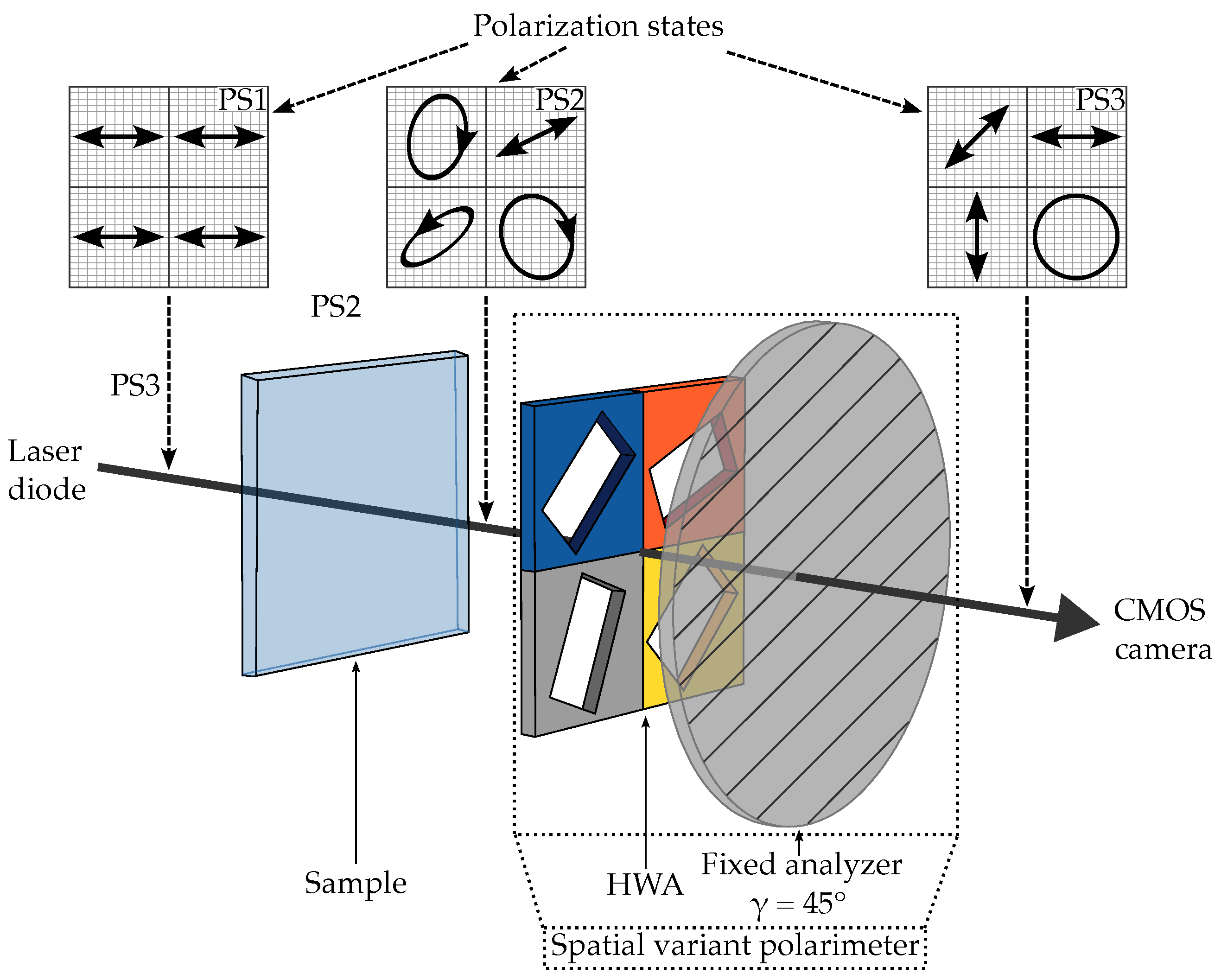
Figure 2.
(top) Schematic illustration of a polarization pixel (enclosed in dotted lines) consisting of four subpixels numbered from I to IV and marked in different colors. Additionally indicated or drawn is the angle as the orientation of the hollow waveguides and the angle , as well as the position of the transmission axis of the analyzer as green dashed lines. (bottom) The schematic drawing shows a single hollow waveguide element in a side view (left) and a top view (right).
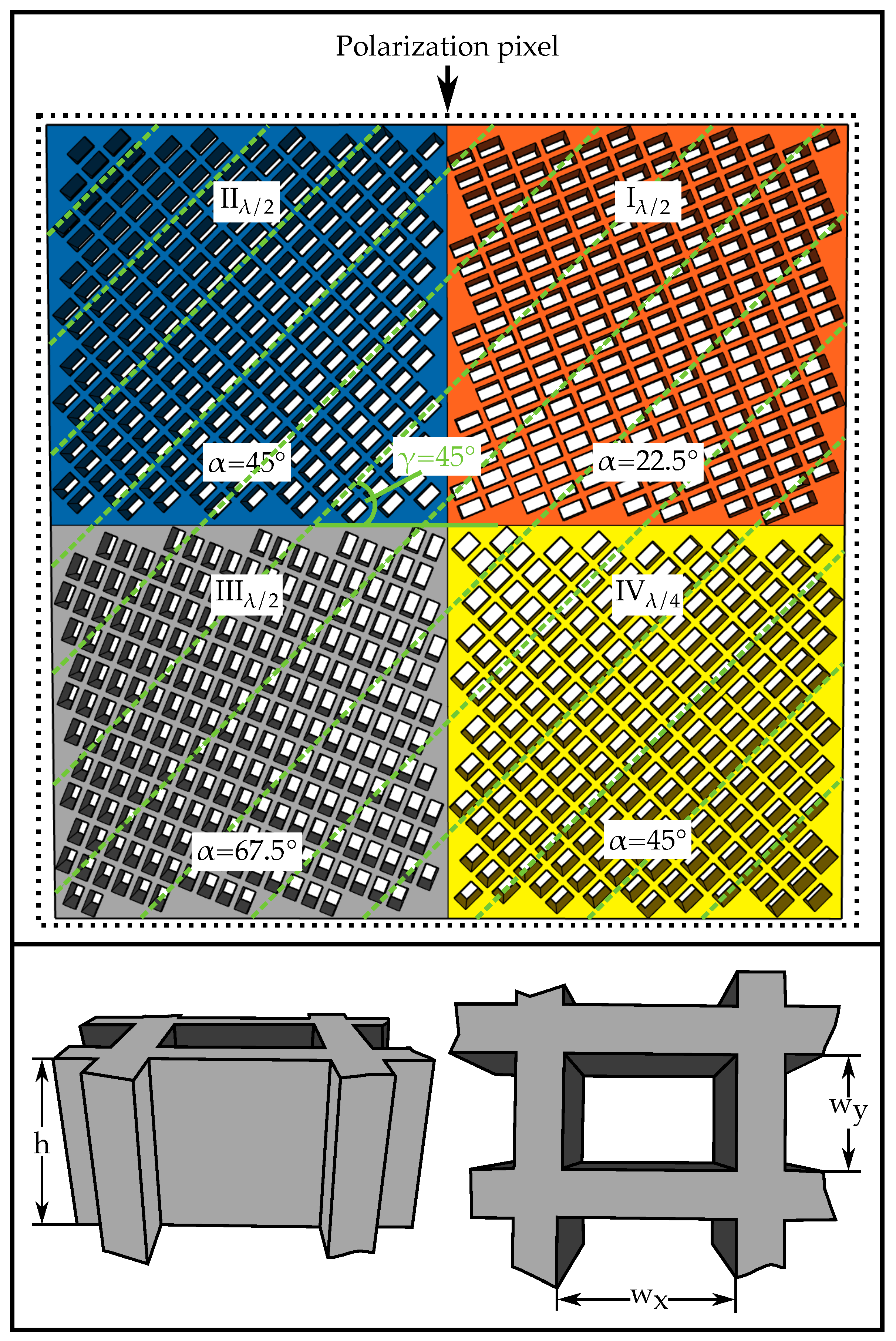
Figure 3.
SEM image of the hollow waveguide array. The left side shows an overview image of several polarization pixels. A single polarization pixel is highlighted by a dashed frame. The right side illustrates a detailed representation of the four different sub-pixels. Comparable to Figure 2, all sub-pixels are additionally indicated.

Figure 4.
Schematic drawing of the experimental setup.

Figure 5.
Intensity distribution of the linear horizontal polarized incident radiation after transmission through the spatial variant polarimeter, captured with the CMOS camera and subsequently normalized to the highest intensity value. The excerpt depicted in the lower image shows the overlapping polarization pixels, as described in the text.

Figure 6.
Spatially resolved Stokes parameters depending on the angular position of a quarter-wave plate.
Figure 6.
Spatially resolved Stokes parameters depending on the angular position of a quarter-wave plate.
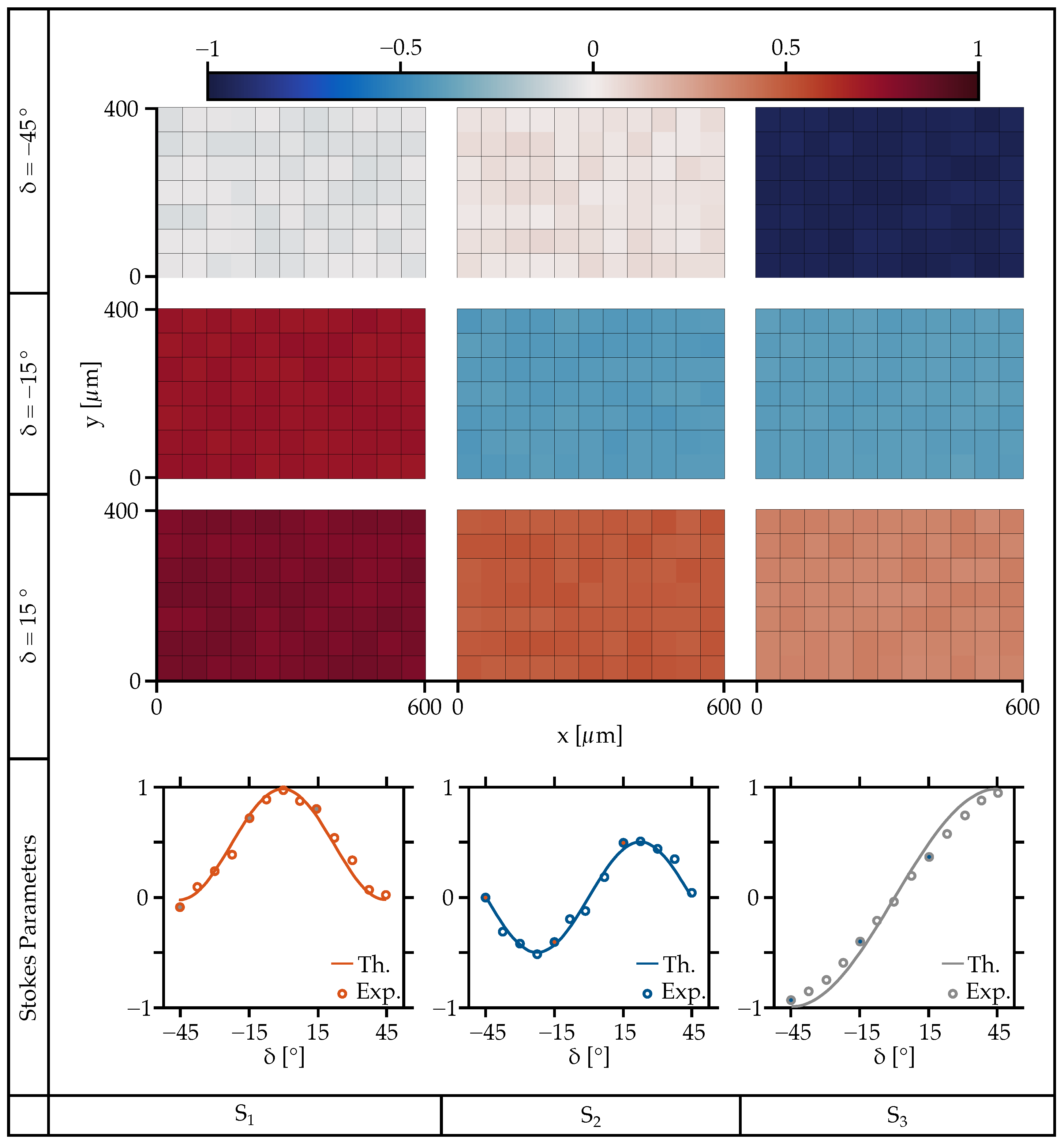
Figure 7.
Spatially resolved Stokes parameters depending on the angular position of a half-wave plate.
Figure 7.
Spatially resolved Stokes parameters depending on the angular position of a half-wave plate.
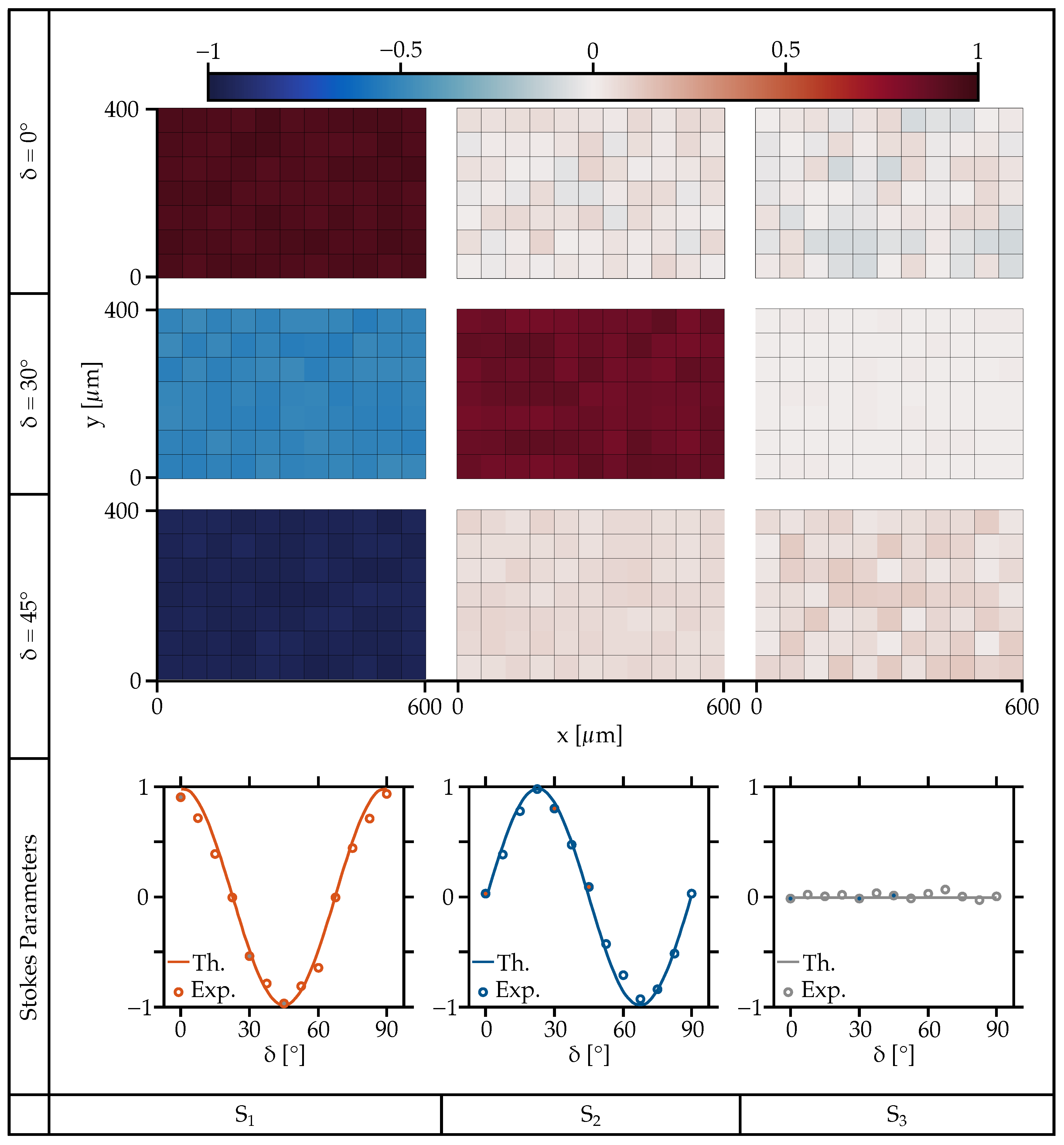
Figure 8.
Top: The figure shows the spatially resolved Stokes parameters of a polymethylmethacrylate plate. Bottom: Comparative polarimetry measurement of the same location on the polymethylmethacrylate plate.
Figure 8.
Top: The figure shows the spatially resolved Stokes parameters of a polymethylmethacrylate plate. Bottom: Comparative polarimetry measurement of the same location on the polymethylmethacrylate plate.

Table 1.
List of parameters for the individual subpixles SPI - SPIV.
| I | 22.5° | 45° | 1550 nm | 872 nm | 45° | |
| II | 45° | 45° | 1550 nm | 872 nm | 90° | |
| III | 67.5° | 45° | 1550 nm | 872 nm | 135° | |
| IV | 45° | 45° | 1550 nm | 1034 nm | 45° |
SP describes the number of the subpixel, the angular orientation of the hollow waveguides, the angle of the analyzer, and the size of the waveguide openings in x and y direction, the resulting angle caused by the phase shift of the half-wave plates, and the intensity value for calculation of the Stokes parameters.
Disclaimer/Publisher’s Note: The statements, opinions and data contained in all publications are solely those of the individual author(s) and contributor(s) and not of MDPI and/or the editor(s). MDPI and/or the editor(s) disclaim responsibility for any injury to people or property resulting from any ideas, methods, instructions or products referred to in the content. |
© 2024 by the authors. Licensee MDPI, Basel, Switzerland. This article is an open access article distributed under the terms and conditions of the Creative Commons Attribution (CC BY) license (https://creativecommons.org/licenses/by/4.0/).
Share and Cite
MDPI and ACS Style
Belle, S.; Kefer, S.; Hellmann, R. Spatially Resolved, Real-Time Polarization Measurement Using Artificial Birefringent Metallic Elements. Photonics 2024, 11, 397. https://doi.org/10.3390/photonics11050397
AMA Style
Belle S, Kefer S, Hellmann R. Spatially Resolved, Real-Time Polarization Measurement Using Artificial Birefringent Metallic Elements. Photonics. 2024; 11(5):397. https://doi.org/10.3390/photonics11050397
Chicago/Turabian StyleBelle, Stefan, Stefan Kefer, and Ralf Hellmann. 2024. "Spatially Resolved, Real-Time Polarization Measurement Using Artificial Birefringent Metallic Elements" Photonics 11, no. 5: 397. https://doi.org/10.3390/photonics11050397
Note that from the first issue of 2016, this journal uses article numbers instead of page numbers. See further details here.