Line-of-Sight Initial Pointing Model of Space Dynamic Optical Network and Its Verification

Abstract

In dynamic space networks, achieving high precision and fast initial pointing of the optical line of sight (LOS) is the key goal in developing this technology. It is the premise and basis of realizing optical LOS capture. Based on the composition and working principle of space optical networking systems, and the effect of real-time position and attitude changes on LOS initial pointing between networks, the matrix transformation and transfer principle is used to establish a multi-link LOS initial pointing model and analyze the factors affecting the size of the field of uncertainty (FOU). In a dynamic space optical networking experiment, the “one-to-two” simultaneous LOS pointing test is carried out, which shows that the model can realize the function of multi-link LOS initial pointing. The sizes of the FOU of the test terminal are 8.67 mrad and 8.34 mrad, respectively, with an average capture time of 18.3 s.

1. Introduction

With the development of space optical technology, the demand for the dynamic networking of optical terminals is increasing. For example, inter-satellite networking optical communication, space optical time–frequency transmission and correction, and space gravitational wave detection have put forward increasingly high requirements for space optical networking systems. Early laser links were mainly “point-to-point”. NASA first launched the “Laser Communications Relay Demonstration Program” [1] to test the capabilities of laser communications at about 22,000 miles from the Earth, conducting two-way laser-link-establishment and communication-demonstration experiments between geosynchronous orbit satellites and Earth.

In 2013, ESA formulated the European Data Relay Satellite plan, which used microwave communications to transmit data between relay satellites and ground stations, and laser links were used to transmit data between relay satellites [2]. With the development of space science and technology, the demand for space networks is increasing day by day. The prerequisite for the application of optical networking is the establishment of network optical links. Russia planned to install spaceborne laser communication equipment on the GLONASS-K series satellites to build a laser communication network among multiple satellites [3]. The low-orbit satellite “Starlink” system performs optical link networking between the same orbit and different orbits to realize the interactive transmission of massive information between backbone networks [4]. In the gravitational wave detector plan, optical links and networks are established between three satellites in solar orbit to form a space triangle interferometer to achieve gravitational wave detection [5]. When a space optical link involves an atmospheric channel, the impact of atmospheric turbulence on the transmission beam cannot be ignored. The Gamma–Gamma model [6], lognormal model [7], etc., can usually be used to describe its power-spectrum distribution characteristics for analysis, and then analyze its impact on boresight capture and tracking accuracy.

As one of the key technologies of space optical networking, LOS initial pointing technology is the prerequisite and a guarantee for various space applications. Reference [8] modified the LOS pointing model and verified its functions and indicators using Terra SAR-X and NFIRE. Taking aircraft-to-ground laser communications as the research background, reference [9] proposed an LOS pointing system that incorporated Kalman filtering technology, which improved the pointing accuracy of LOS pointing, but also reduced the size of the FOU of the LOS from 10.06 mrad to 5.06 mrad. Reference [10] proposed a dynamic initial pointing algorithm based on an integrated GPS/INS navigation system, and designed a hardware system for outdoor verification of the algorithm. The correctness and reliability of the pointing system were analyzed.

This article studies the principle and implementation method of laser-link building between space networks based on existing “point-to-point” laser-link building techniques. Based on the impact of real-time position and attitude changes on the LOS pointing, and through the principle of coordinate conversion and transfer, a “point-to-multipoint” multi-link LOS initial pointing model was established. We completed model verification and indicator testing in the dynamic space optical networking test.

2. Optical Networking System Composition and Working Principle

The principles of “point-to-multipoint” laser networking are shown in Figure 1. The optical antenna of the optical terminal is based on a rotating parabola, and several mirrors are spliced together to form a pointing mechanism. The rotating parabola has an optical property whereby the reflected light is parallel to the rotational symmetry axis of the paraboloid when the incident light passes through the focus. The normal line of each mirror is perpendicular to the tangent line of the paraboloid. Each mirror can be controlled to move in terms of azimuth and elevation, meaning that the antenna has certain light stabilization and deflection functions and can establish multiple optical links based on azimuth and elevation direction at the same time.

The multiple mirrors of the optical terminal are uniformly arranged around the optical terminal, where each mirror is responsible for designing the capture range of the space. For example, the four mirrors capture a range covering 360°. Each mirror has an azimuth capture range of 90° and an elevation capture range of 0–30°. The azimuth–elevation frame can adjust the pointing angle of the optical antenna by adjusting the optical LOS attitude of the mirror, so as to realize multi-link LOS pointing to the FOU. After capture and tracking, the precise alignment of the LOS is realized. Then, communication, distance measurement, time–frequency transmission, and other functions can be carried out between space networks.

3. Multi-Link LOS Pointing Model

3.1. The Principle of LOS Pointing

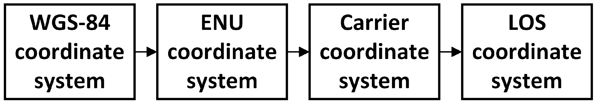
As shown in Figure 1, when the space optical terminal is used in dynamic applications, it is necessary to compensate for changes in the position and attitude of the optical terminal in real time to achieve multi-link optical pointing. After a series of coordinate conversion and transfer processes, we used the multi-link LOS initial pointing model, established based on the point-to-point LOS initial pointing model, to obtain the azimuth and elevation angles required to rotate the LOS of each mirror relative to its initial zero position [9]. Applying the coordinate transformation matrix requires the clarification of the number of coordinate systems, the order of the coordinate systems, and the positive and negative standards for rotation angles. It should be noted that the same standard must be used for each coordinate system.

3.1.1. Coordinate System Definition

WGS-84 coordinate system e: With the center of mass of the earth as the coordinate origin, the Z-axis is found along the polar axis, the X-axis is located at the intersection of the prime meridian and the equatorial plane, and the Y-, Z-, and X-axes form a right-handed coordinate system.

East–north–up (ENU) coordinate system: Taking the station center or terminal center as the origin, the X-axis points east along the local latitude, the Y-axis points north along the local meridian, and the Z-, X-, and Y-axes form a right-handed coordinate system.

Carrier coordinate system b: This coordinate system is concentric with the northeast celestial coordinate system. The X-axis is located to the right along the horizontal axis of the carrier, the Y-axis is found to the front along the vertical axis of the carrier, and the Z-axis is perpendicular to the X-axis and the Y-axis, forming a right-handed coordinate system.

LOS coordinate system: Taking the center of the optical antenna as the origin, the r-axis is found along the optical LOS of the capture antenna, e points along the distance direction, the d and r-axes are orthogonal axes, and the three axes r, e, and d form a right-handed coordinate system.

Since the networking system is a multi-LOS system, there are multiple LOS coordinate systems, and the relationship between each LOS coordinate system and the carrier coordinate system needs to be calibrated in advance.

3.1.2. Coordinate Conversion and Transfer Principle

• Geodetic Coordinate–Rectangular Coordinate Conversion

Before performing coordinate conversion, it is necessary to convert the geodetic polar coordinates into rectangular coordinates, that is, to convert the longitude, latitude, and altitude into rectangular coordinate values. The ellipsoid parameters are selected according to the WGS-84 ellipsoid model, and the conversion formula is shown in Formula (1):

$$\left(\begin{array}{c}{X}_{o,i}\\ Y_{o,i}\\ Z_{o,i}\end{array}\right)=\left(\begin{array}{c}(N+H_{o,i})\cos B_{o,i}\cos L_{o,i}\\ (N+H_{o,i})\cos B_{o,i}\sin L_{o,i}\\ (N(1-e^2)+H_{o,i})\sin B_{o,i}\end{array}\right)$$

(1)

where $N=\frac{a}{\sqrt{1-e^2{(\sin B_{o,i})}^2}}$; ellipsoid long radius $\mathrm{a}=6378137\mathrm{m}$; and eccentricity squared $e^2=0.006694379995$. $B_{o,i},L_{o,i},H_{o,i}$ are the longitude, latitude, and altitude values, obtained in real time. The subscript o represents one’s own side, and the subscript i represents the other party of the i link, where i = 1, 2, 3, 4….

2.

Matrix transfer principle [9]

The i-th LOS conversion and transmission principle is shown in the Figure 2.

The conversion matrix used to convert the coordinates in the opponent’s WGS-84 coordinate system to the coordinates in the east–north–up coordinate system with one’s own side as the origin is as follows:

$$C_e^n=\left(\begin{array}{ccc}-\sin L_o& \cos L_o& 0\\ -\sin B_o\cos L_o& -\sin B_o\sin L_o& \cos B_o\\ \cos B_o\cos L_o& \cos B_o\sin L_o& \sin B_o\end{array}\right)$$

(2)

$C_e^n$ real-time compensation for the impact of changes in one’s own position on the pointing model. Among them, $B_o,L_o,H_o$ are the longitude, latitude, and altitude values of the origin in the east–north–up coordinate system, which are obtained in real time by one’s own position sensor.

The conversion matrix used to convert the coordinates in the opponent’s east–north–up coordinate system into the coordinates in the carrier coordinate system, with one’s own side as the origin, is as follows:

$$C_n^{\mathrm{b}}=\left(\begin{array}{ccc}\cos r\cos y-\sin r\sin p\sin y& \cos r\sin y+\sin r\sin p\cos y& -\sin r\cos p\\ -\cos p\sin y& \cos p\cos y& \sin p\\ \sin r\cos y+\cos r\sin p\sin y& \sin r\sin y-\cos r\sin p\cos y& \cos p\cos r\end{array}\right)$$

(3)

$C_n^{\mathrm{b}}$ is real-time compensation for the impact of changes in one’s own heading angle, pitch angle, and roll angle on the pointing model, where y, p, and r, respectively, represent one’s own real-time heading angle, pitch angle, and roll-angle values, which are obtained in real time from one’s own attitude sensor. The angle range of heading angle rotation is from 0 degrees to 360 degrees. The angle range of pitch angle rotation is from −90 degrees to +90 degrees. The angle range of roll-angle rotation is from −90 degrees to +90 degrees.

Definition of the conversion matrix that converts the coordinates in the opponent’s carrier coordinate system into the coordinates in the i-th visual-axis coordinate system, with one’s own side as the origin, is as follows:

$$C_{bi}^a=\left(\begin{array}{ccc}\cos {\theta }_{xi}\cos {\theta }_{yi}-\sin {\theta }_{xi}\sin {\theta }_{zi}\sin {\theta }_{yi}& \cos {\theta }_{xi}\sin {\theta }_{yi}+\sin {\theta }_{xi}\sin {\theta }_{zi}\cos {\theta }_{yi}& -\sin {\theta }_{xi}\cos {\theta }_{zi}\\ -\cos {\theta }_{zi}\sin {\theta }_{yi}& \cos {\theta }_{zi}\cos {\theta }_{yi}& \sin {\theta }_{zi}\\ \sin {\theta }_{xi}\cos {\theta }_{yi}+\cos {\theta }_{xi}\sin {\theta }_{zi}\sin {\theta }_{yi}& \sin {\theta }_{xi}\sin {\theta }_{yi}-\cos {\theta }_{xi}\sin {\theta }_{zi}\cos {\theta }_{yi}& \cos {\theta }_{zi}\cos {\theta }_{xi}\end{array}\right)$$

(4)

$C_{bi}^a$ compensates for the effect of differences between the different axes of view on the pointing model. ${\theta }_{xi}$, ${\theta }_{yi}$, and ${\theta }_{zi}$ are the angles between the three coordinate axes of the i-th LOS coordinate system and the carrier coordinate system. These are known values which are measured and calibrated during installation. If four coordinate systems of LOS are established in the same plane at the same time, ${\theta }_{x1}$ = ${\theta }_{y1}$ = 0°; ${\theta }_{x2}$ = ${\theta }_{y2}$ = 90°; ${\theta }_{x3}$ = ${\theta }_{y3}$ = 180°; ${\theta }_{x4}$ = ${\theta }_{y4}$ = 270°; ${\theta }_{z1}$ = ${\theta }_{z2}$ = ${\theta }_{z3}$ = ${\theta }_{z4}$ = 0°.

3.1.3. Pointing Angle Calculation

After the above coordinate conversion, the coordinates $\left(x_i,y_i,z_i\right)$ of the i-th opponent (coordinates in the WGS-84 coordinate system) in one’s own sight-axis coordinate system can be obtained. The calculation formula is as follows:

$$\left(\begin{array}{c}{x}_i\\ y_i\\ z_i\end{array}\right)=C_{bi}^a{C}_n^b{C}_e^n\left(\begin{array}{c}{X}_o-X_i\\ Y_o-Y_i\\ Z_o-Z_i\end{array}\right)$$

(5)

In the formula, $X_o,Y_o,Z_o$ and $X_i,Y_i,Z_i$ are the master–slave terminal geodetic rectangular coordinate values obtained by substituting the longitude, latitude, and elevation values into Equation (1).

The initial pointing angle of the visual axis is defined in the visual-axis coordinate system and can be calculated by the following formula:

$$\left\{\begin{array}{l}{\alpha }_i=\arctan (x_i/y_i)\hfill \\ {\beta }_i=\arctan (z_i/\sqrt{x_i^2+y_i^2})\hfill \end{array}\right.$$

(6)

In the formula, respectively, the i-th visual axis needs to rotate around the azimuth angle and elevation angle. The formula shows the coordinates of the opponent’s coordinate point (coordinates under WGS-84) in relation one’s own i-th visual-axis coordinate system.

3.2. FOU

Various factors limit the accuracy of the initial pointing. In addition, there are errors in the azimuth axis and elevation axis. The errors of the two axes are independent of each other and follow a Gaussian distribution, with a mean of zero. The error of the initial pointing angle is a Rayleigh distribution, which can be expressed as follows [11]:

$$f({\theta }_i)=\frac{1}{\sqrt{2\pi {\sigma }_i}}\exp \left(-\frac{{\theta }_i^2}{2{\sigma }_i^2}\right)$$

(7)

where ${\theta }_i=\sqrt{{\theta }_{{\alpha }_i}^2+{\theta }_{{\beta }_i}^2}$ is the initial pointing error angle, ${\theta }_{{\alpha }_i}$ is the azimuth direction error angle, ${\theta }_{{\beta }_i}$ is the elevation direction error angle, and ${\sigma }_i$ is the standard deviation of the initial pointing error angle, that is, the pointing error. If the Gaussian distribution has the same standard deviation, ${\sigma }_i$ = ${\sigma }_{{\alpha }_i}$ = ${\sigma }_{{\beta }_i}$, in the azimuth direction error angle and the elevation direction error angle, then the path i capture probability is as follows:

$$P_i={\displaystyle \int {\displaystyle {\int }_{FO{U}_i}\frac{1}{\sqrt{2\pi }{\sigma }_i}}}\exp \left(-\frac{{\theta }_{{\alpha }_i}^2}{2{\sigma }_i^2}\right)\times \frac{1}{\sqrt{2\pi }{\sigma }_i}\exp \left(-\frac{{\theta }_{{\beta }_i}^2}{2{\sigma }_i^2}\right)\mathrm{d}{\theta }_{{\alpha }_i}\mathrm{d}{\theta }_{{\beta }_i}$$

(8)

Formula (8) is simplified to a uniform distribution with pole angle $1/2\pi$, and the integral in the polar coordinate system is as follows:

$$P_i={\displaystyle {\int }_0^{FO{U}_i/2}\frac{{\theta }_i}{{\sigma }_i^2}}\exp \left(-\frac{{\theta }_i^2}{2{\sigma }_i^2}\right)\mathrm{d}{\theta }_i$$

(9)

Because of the pointing error, LOSs will not accurately point to each other, but to FOU. For a capture probability greater than 98.89%, $P_i\ge 98.89\%$, $FO{U}_i\ge 3{\sigma }_i$ is calculated. It can be seen that the size of FOU is determined by the pointing error. There are many factors affecting the pointing error, including position error, attitude error, dynamic lag, platform vibration, LOS stability error, and alignment error of system instrument installation.

When the optical terminal between the network nodes is in a state of follow-up pointing, the pointing error can be obtained using the azimuth and elevation follow-up pointing angle, and then the size of FOU can be obtained. The azimuth error angle ${\theta }_{{\alpha }_i}$ can be obtained by determining the difference between the measured azimuth angle ${\alpha }_i^m$ and the theoretical value ${\alpha }_i$, calculated using the above pointing model, and ${\sigma }_{{\alpha }_i^2}$ can be obtained according to the following formula. Similarly, ${\theta }_{{\beta }_i}={\beta }_i^m-{\beta }_i$ is calculated according to the following formula to obtain ${\sigma }_{{\beta }_i^2}$. The calculation formula is as follows:

$${\sigma }_{{\chi }_i^2}=\frac{\sum {({\theta }_{{\chi }_i}-{\mu }_{{\chi }_i})}^2}{N_{{\chi }_i}}$$

(10)

The size of FOU of the i route can be obtained, and deduced the formula is as follows:

$$FO{U}_i=3{\sigma }_i=3\sqrt{{\sigma }_{{\alpha }_i^2}+{\sigma }_{{\beta }_i^2}}$$

(11)

4. Experimental Results and Analysis

In the “one-to-two” simultaneous laser communication demonstration test, the multi-link LOS initial pointing networking model is verified. The principle of the networking system is shown in Figure 3. The experimental system consists of three parts: the master optical terminal, the slave optical terminal 1 (airship), and the slave optical terminal 2 (ground terminal). The master optical terminal (as shown in Figure 4a) can simultaneously point to, capture, and build a chain for the airship (as shown in Figure 4b) and the ground optical terminal. The link distance between the master optical terminal and the slave optical terminal is 2 km. Testing space optical networking technology performance and indicators involves the pointing accuracy, the size of FOU, the communication rate, and the BER. Due to the conditions of the test site, the flying height of the airship is 200 m.

The main technical parameters of the master and slave optical terminals are shown in

Table 1. Main technical parameters of master–slave optical terminals.

Device Parameters	Master Optical Terminal	Slave Optical Terminals
Beacon light emission band	730 nm	785 nm
Beacon light receiving band	785 nm	730 nm
Beacon beam divergence	2 mrad	1 mrad
Optical aperture	186 mm	90 mm
Detection field of view	7 mrad	7 mrad

.

The master optical terminal, slave optical terminal 1, and slave optical terminal 2 are equipped with dual-antenna integrated GPS/INS navigation and positioning system to provide the necessary positional and attitude information for the LOS pointing model. The position positioning accuracy is better than 1.5 m, and the attitude accuracy is 0.1°. The position coordinates of the three terminals in the experiment are shown in

Table 2. GPS position of master and slave optical terminals.

Position	Longitude (deg)	Latitude (deg)	Altitude (m)
Master optical terminal	94.73965454	29.72693825	3412.197998
Slave optical terminals 1	94.72811127	29.7315197	3355.039063
Slave optical terminals 2	94.74954426	29.71982796	3411.265796

.

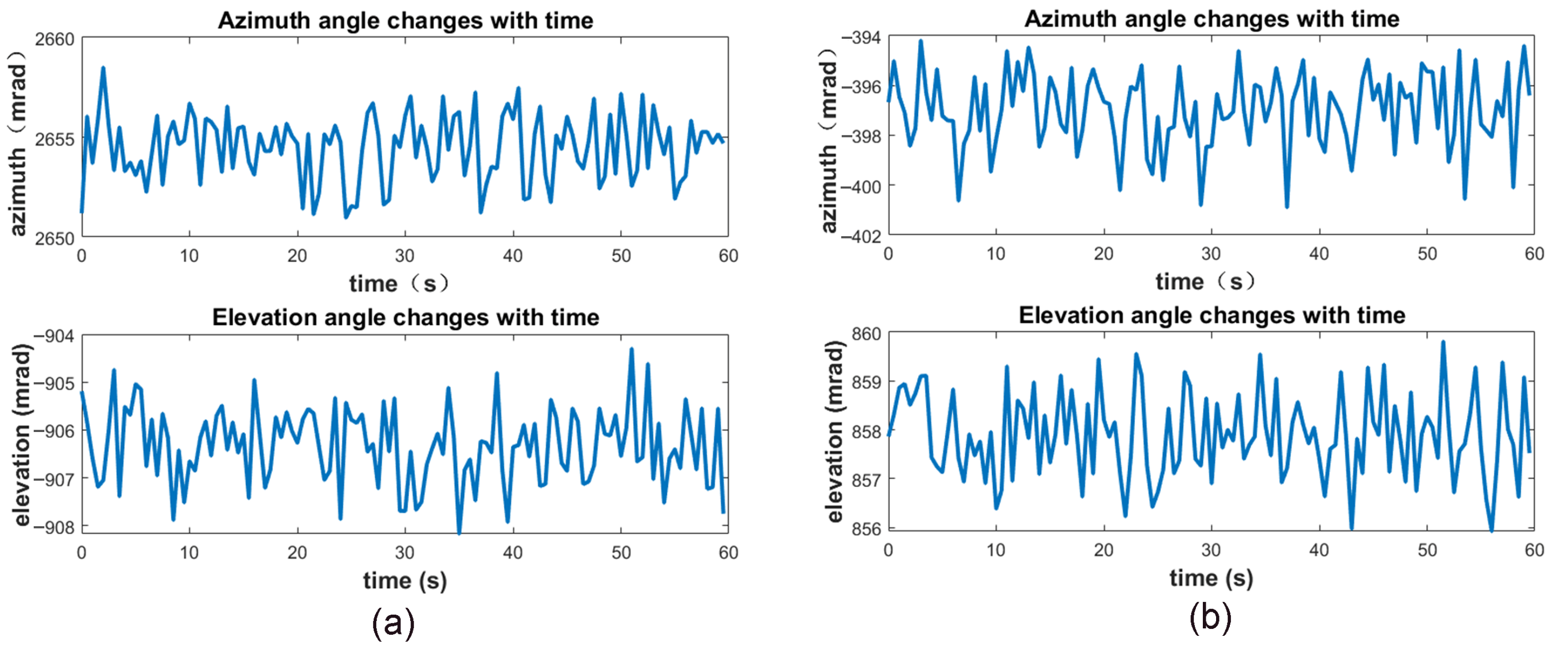
In the pointing model test, three optical terminals open the LOS initial pointing unit at the same time to establish two optical links. The terminal of each link calculates the initial pointing angle in relation to the opposite end according to its own attitude angle, position, and the position of the other side terminal, and the corresponding angle of the rotation of the optical LOS points to the FOU. The size of the FOU was measured during the experiment. When the two mirrors of the main optical terminal were in the follow-up pointing state, the magnitude changes of their respective azimuth and elevation angle were recorded, and the results are shown in Figure 5. The sampling time was 60 s, and the sampling frequency was 2 Hz.

We performed statistical processing on the azimuth and elevation angles of the two mirrors to be rotated, and results recorded are shown in Figure 5. A data statistics histogram was obtained, as shown in Figure 6. Figure 6a,b show the azimuth and elevation angle data of the master optical terminal pointing to slave optical terminal 1. Figure 6c,d are the azimuth and elevation angle data of slave optical terminal 2.

The experiment was conducted in the atmospheric channel, and link establishment was completed using a coarse–fine composite axis structure. The tracking accuracy of the coarse tracking system was 50 μ rad. The impact of turbulence on the tracking accuracy was generally between 5–25 μ rad. Moreover, the position of the airship changed very little during the experiment, and the dynamic lag error was very small. Therefore, the recorded azimuth and elevation angle statistics basically obeyed Gaussian distribution. The data shown in Figure 6 were statistically processed according to Equation (10), and the pointing errors and FOU were obtained as follows. The variance in the azimuth angle and elevation angle of the master optical terminal pointing to slave optical terminal 1 was 2.82 mrad and 0.64 mrad, respectively. The variance in the azimuth and elevation angle of the master optical terminal pointing to slave optical terminal 2 was 2.68 mrad and 0.71 mrad, respectively. The pointing error ${\sigma }_1$ was $\sqrt{{2.82}^2+{0.64}^2}=2.89 \mathrm{mrad}$ when pointing to the slave optical terminal 1, and ${\sigma }_2$ was $\sqrt{{2.68}^2+{0.71}^2}=2.78 \mathrm{mrad}$ when pointing to the slave optical terminal 2. The sizes of FOU were 2.89 × 3 = 8.67 mrad and 2.78 × 3 = 8.34 mrad, respectively.

The gaze + scan method was used for scanning and capturing. The scanning mode was spiral scanning, the scanning dwell time was 0.1 s, and the overlap factor was 0.3. After optical LOS scanning, an optical link was established. The 20 LOS pointing and capturing experiments were all successful, and the average scanning time was 18.3 s. The successful capture of the two links verified the correctness and feasibility of the initial pointing model of the spatial dynamic optical network’s LOS.

5. Discussion

Whether an LOS can be correctly rotated in relation to the FOU determines whether an optical link can be established, and the size of the FOU determines the length of the optical link’s establishment time. This is not only the key to successful capture, but is also key to the premise and guarantee of optical link networking. This paper establishes a multi-link LOS initial pointing model, determines the factors that affect the size of the FOU, and proposes an FOU calculation method based on the pointing azimuth angle variance and elevation angle variance. In the “one-to-two” simultaneous LOS pointing demonstration test, the size of the multi-link FOU was tested, the correctness of the pointing model was verified, and these results laid the foundation for subsequent multi-link fast beam scanning and capture. Consequently, through structural optimization design, signal filtering and prediction, high-precision position and attitude sensors and other methods can be used to improve the LOS pointing accuracy, reduce the size of the FOU, and reduce the overall capture time. The space multi-link LOS pointing method being studied is universal. Based on the corresponding space optical network application scenarios, it can be applied to inter-satellite laser network communications, time–frequency transmission, laser ranging, gravitational wave detection and other related fields in order to achieve optical network LOS pointing and correction, determine the size of the FOU, provide time analysis, etc. It provides a corresponding reference for the establishment of space optical networking links.

References

- Israel, D.J.; Edwards, B.L.; Staren, J.W. Laser Communications Relay Demonstration (LCRD) update and the path towards optical relay operations. In Proceedings of the 2017 IEEE Aerospace Conference, Big Sky, MT, USA, 4–11 March 2017; pp. 1–6. [Google Scholar]
- Gregory, M.; Heine, F.; Kämpfner, H.; Lange, R.; Lutzer, M.; Meyer, R. Commercial optical inter-satellite communication at high data rates. Opt. Eng. 2012, 51, 031202. [Google Scholar] [CrossRef]
- Kumar, P.; Srivastava, P.K.; Tiwari, P.; Mall, R.K. Chapter 20—Application of GPS and GNSS technology in geosciences. GPS Solut. 2018, 22, 1–14. [Google Scholar]
- McDowell, J.C. The Low Earth Orbit Satellite Population and Impacts of the SpaceX Star link Constellation. Astrophys. J. Lett 2020, 892, L36. [Google Scholar] [CrossRef]
- Luo, Z.; Wang, Y.; Wu, Y.; Hu, W.; Jin, G. The Taiji program: A concise overview. Prog. Theor. Exp. Phys. 2021, 2021, 05A108. [Google Scholar] [CrossRef]
- Kashani, M.A.; Uysal, M.; Kavehrad, M. A Novel Statistical Channel Model for Turbulence-Induced Fading in Free-Space Optical Systems. J. Light. Technol. 2015, 33, 2303–2312. [Google Scholar] [CrossRef]
- Karimi, M.; Nasiri-Kenari, M. BER Analysis of Cooperative Systems in Free-Space Optical Networks. J. Light. Technol. 2009, 27, 5639–5647. [Google Scholar] [CrossRef]
- Fields, R.; Lunde, C.; Wong, R.; Wicker, J.; Kozlowski, D.; Jordan, J.; Hansen, B.; Muehlnikel, G.; Scheel, W.; Sterr, U.; et al. NFIRE-to-Terra SAR-X laser communication results: Satellite pointing, disturbances, and other attributes consistent with successful performance. In Proceedings of the SPIE Defense, Security, and Sensing, Orlando, FL, USA, 13–17 April 2009; Volume 7330. [Google Scholar]
- Wu, R.; Zhao, X.; Liu, Y. Initial Pointing Technology of Line of Sight and its Experimental Testing in Dynamic Laser Communication System. IEEE Photonics J. 2019, 11, 7903008. [Google Scholar] [CrossRef]
- Yang, B.; Wang, J.; Wang, J. Verification of dynamic initial pointing algorithm on two-dimensional rotating platform based on GPS/INS. Proc. SPIE 2015, 9671, 967107. [Google Scholar]
- Li, X.; Yu, S.; Ma, J.; Tan, L. Analytical expression and optimization of spatial acquisition for intersatellite optical communications. Opt. Express 2011, 19, 2381–2390. [Google Scholar] [CrossRef] [PubMed]
Figure 1.
Composition principle of space optical networking optical terminal.
Figure 2.
Coordinate conversion and transfer process.
Figure 3.
“One-to-two” optical networking test principle.
Figure 4.
Physical image of master optical terminal and airship: (a) physical image of master optical terminal; (b) physical image of airship.
Figure 5.
Recorded data of azimuth and elevation changes of the mirror under the direction of follow-up: (a) pointing to slave optical terminal 1; (b) pointing to slave optical terminal 2.
Figure 6.
Statistical histogram of azimuth and elevation angle data. (a) Statistical histogram of azimuth angle data pointing to slave optical termina 1; (b) Statistical histogram of elevation angle data pointing to slave optical termina 1; (c) Statistical histogram of azimuth angle data pointing to slave optical termina 2; (d) Statistical histogram of elevation angle data pointing to slave optical termina 2.