Coupled CFD-Response Surface Method (RSM) Methodology for Optimizing Jettability Operating Conditions

Abstract

A volume-of-fluid (VOF) finite volume model under the ANSYS^® Fluent framework was coupled with the response surface method (RSM) to find the best operating conditions within a jettability window for two selected responses in a drop-on-demand inkjet printing process. Twenty-five runs were generated using a face centred design and numerical simulations were carried out using viscosity, surface tension, nozzle diameter, and inlet velocity as input factors. A mesh study was first conducted to establish the necessary number of cells to best combine accuracy and expended time. Selected runs were discussed, identifying the underpinning mechanisms behind the droplet generation at different time periods. Each one of the responses was evaluated under different input factors and their effects were identified. Finally, the desirability function concept was advantageously used to proceed with a multiple optimization where all the responses were targeted under usual jettability/printability conditions.

1. Introduction

Droplets generation understanding is of crucial importance in several industrial applications [1]. Inkjet printing processes are characterized by a unique and small droplet size, typically ranging from 10 to 100 μm [1] and can be obtained using a continuous or an impulsive flow (the last one is also known as drop-on-demand (DoD) inkjet). Thanks to several advantages, the DoD method is gaining considerable acceptance in industrial environments [2].

DoD is a complex process and depends on several parameters that fall into three main categories: fluid properties, nozzle geometry, and driving waveform [1,3].

However, experiments are hard to get because both length and time scales are in the micro order [4]. As a consequence, experimental set-ups are always expensive and complex, with advanced numerical approaches such as computational fluid dynamics (CFD) being a strict requirement [5,6]. The volume-of-fluid (VOF) approach is found to be a proper alternative to simulate a multiphase process on liquid break-up and droplet generation and has been used as such in past research [7,8], with the former, in the context of printing processes, still being a subject of present research. Also, the VOF scheme allows to effectively simulate two or more immiscible fluids with a clearly defined interface by solving a single set of momentum equations and tracking the volume fraction of each of the fluids throughout the domain. Feng [9] performed one of the pioneer works simulating the complex fluid dynamic process during drop ejection using the package FLOW-3D, which employs the VOF approach to effectively track the transient fluid interface deformations and disruptions. The main goal was the implementation of general design rules in device development, with a better understanding of sensitive variables such as volume and speed.

One of the major questions related to this kind of processes is the definition of an operating range for a stable drop formation. Fromm [10] established that when the ratio of the Reynolds number to the square root of the Weber number is less than 2, it is impossible to generate stable drops. This dimensionless value was later known as the Z number and defines a jettability range [11]. From the literature, different Z intervals for jettability purposes, ranging from 1 to 10 [12], 4 to 14 [13], or even 0.67 to 50 [14], can be found. This clearly means that the Z value alone is not able to indicate the jettability conditions. Indeed, fluids with different properties could present the same Z value while showing different printing quality.

The droplet generation process and corresponding jettability is mainly determined by a set of parameters that have a strong influence on the overall process quality. A better understanding of the underpinning mechanisms requires performing several experimental or numerical runs considering an extended set of operating conditions and parameters. Without a systematic approach, such as the design-of-experiment (DoE) approach, this can become an extremely hard task to accomplish.

Since the pioneer article from Box and Wilson [15], where, for the first time, a systematized approach was developed using response surface methods to solve optimization problems, this proven methodology has been applied successfully to a large number of chemical and other related academic and industrial processes [16]. For instance, Silva and Rouboa [17] used a response surface methodology (RSM) to identify the relevant parameters affecting the power density of a direct methanol fuel cell.

In many real industrial applications, experimental studies are limited because of the difficulty of regulating the operating parameters, but mainly because of the high cost of developing set-ups or running the experiments. Therefore, the solution relies on the development of effective mathematical models able to simulate and predict the main system responses. Combining optimization methodologies such as DoE with numerical models avoids expensive and time-consuming experiments, while allowing for obtaining optimal conditions using different input combinations [16]. Silva and Rouboa [18] coupled the results obtained from a 2D Eulerian–Eulerian biomass gasification model, developed under the CFD framework, with RSM to find the best operating conditions to generate syngas for different applications. The authors were able to find the operation conditions that guaranteed both the best response and minimal variations caused by input factors. Frawley et al. [19] combined CFD and DoE techniques (RSM in particular) to examine the effect of varying key factors on solid particle erosion in elbows in pipes, allowing them to develop an erosion prediction model.

To the best of our knowledge, there are no studies implementing the DoE approach (experimentally or combined with any kind of numerical models) applied to the improvement and better understanding of a DoD inkjet process. It is likely that leading companies may be applying these kinds of approaches, but related results maybe sensitive and thus are not made available to the wider community. This fact could increase the impact of present paper, as a study of this kind, aimed at evaluating the effect of several parameters on the droplet generation in DoD inkjet process.

By using a VOF approach within the CFD framework, a design of several computer experiments was developed and RSM was used as an analysis tool. A mesh convergence study was performed in order to balance sufficient numerical accuracy with an acceptable time computing simulation. For design purposes, viscosity, surface tension, inlet velocity, and nozzle diameter were selected as input factors. The responses were break-up time and break-up length.

2. Materials and Methods

2.1. Problem Description

To properly test the hypothesis that RSM is a suitable tool for predicting the jettability range, one needs to create a computational domain in which the governing equations are solved. Regarding DoD devices, their configuration can greatly vary to accommodate the specific actuation method and the fluid dynamics of drop ejection (especially near the nozzle region), but is essentially the same [9]. For that reason, the present study focuses on a rather idealized, generic fluid chamber configuration, as shown in Figure 1.

Dimensions of the computational domain are summarized in

Table 1. Geometry dimensions.

Ink Chamber, Cylindrical Region	Radius (mm) 0.011–0.021
Ink Chamber, Cylindrical Region	Length (mm) 0.050
Ink Chamber, Tapered Region	Final Radius (mm) 0.005–0.015
Ink Chamber, Tapered Region	Length (mm) 0.050
Air Chamber	Radius (mm) 0.030
Air Chamber	Length (mm) 0.280

. The radius for both the cylindrical and tapered regions for the ink chamber appears as a range instead of a fixed value because its influence is going to be analysed in a later chapter.

The ink jetting process is activated by an electrical pulse, generating a high pressure inside the nozzle, forcing the liquid to start to flow out of the orifice [3]. To replicate this process, a time-dependent velocity boundary condition is prescribed at the nozzle inlet. Before the process starts, the nozzle is filled with ink, while the rest of the domain is filled with air. To initiate the ejection, the ink velocity at the inlet boundary suddenly increases from zero to maximum velocity, and then decreases according to a cosine law. After 10 microseconds, the velocity returns to zero. This can be easily accomplished by a user-defined function.

2.2. Model Implementation

To obtain a reasonable solution within an acceptable timeframe, there are several basic assumptions one must follow. To begin, laminar flow is an appropriate assumption when dealing with droplet generation with small geometries, droplet diameters, and overall low velocities (thus resulting in a relatively low Reynolds number). By following this assumption, one can also assume that there is no swirl generated in the fluid and, therefore, the azimuthal direction flow is absent. By doing so, one can assume that the jet is axisymmetric and that it can be fully described by a 2D coordinate system consisting of an axial coordinate z and a radial coordinate r [20].

As only an infinitesimal air amount will be moved by the droplets (most of the surrounding air is still) and, as stated, the velocity is relatively slow and the Mach number is definitely below 0.3, one can assume the air in the chamber as being incompressible.

A well-known numerical study on drop formation using ANSYS^® Fluent was used as a starting block to conduct this study [21]. Improvements were attained by means of several user-defined functions. As our model faithfully represents what other authors have obtained, it is reasonable to assume the model will still be appropriate with add-ins from our own operational conditions.

2.3. Grid Selection Study

Numerical methods require the geometry to be broken into discrete cells. This process is known as meshing or discretization. The ability of numerical methods to accurately predict results relies upon the mesh quality.

Because of the simplicity of the described geometry, a quadrilateral mesh was generated using a non-uniform grid to discretize the domain. The mesh near the symmetry axis was kept very fine as compared with the rest of the domain, where the gradients were large. This helped in reducing the number of cells and hence the computational time. Grid independence studies help to avoid the use of an excessive number of cells, while preserving the accuracy of the final solution. Simulations were carried out on four different grids with increasing grid density in order to ensure a grid-independent solution.

Table 2. Mesh characteristics.

Mesh	Face Size	Number of Elements
1	1 mm	9331
2	0.750 mm	16,707
3	0.625 mm	23,978
4	0.550 mm	30,658

displays the main characteristics of each mesh.

To select the appropriate grid, one must choose a particular set of results, analyse results for all meshes, and make a compromise between accuracy and computational cost. As we are interested in the drop formation itself, the major result we are interested is the liquid fraction contour. Figure 2 shows the ink fraction contours at the following four time steps: 6 μs, 12 μs, 18 μs, and 24 μs.

The results show that by increasing mesh density, the model is able to better capture the interface between liquid and gas phases. Similar results were found for different parameters and for additional time steps. The global run-time for mesh 1 reaches the one-hour mark, while meshes 2 and 3 finish just shy of two hours. The fourth mesh took slightly under three hours to complete. This presents a very interesting conclusion on how important grid independence studies actually are. Mesh 3 gives close results when compared with mesh 4, saving about one hour in each run. Mesh 3 was selected for this work as it presents the best commitment between results accuracy and expended computational time.

3. Mathematical Model

Following the assumptions made in the previous section, the multiphase incompressible Navier–Stokes equations are adequate to model the flow when the viscous liquid is ejected. Assuming axial symmetry, they take the following form for each phase:

$$\frac{\partial u_r}{\partial t}+\frac{\partial \left(r{u}_r{u}_z\right)}{r\partial z}+\frac{\partial \left(r{u}_r{u}_r\right)}{r\partial r}=-\frac{1}{\rho }\left(\frac{\partial p}{\partial r}\right)+\frac{\mu }{\rho }\left(\frac{{\partial }^2{u}_r}{\partial r^2}+\frac{1}{r}\frac{\partial u_r}{\partial r}+\frac{{\partial }^2{u}_r}{\partial z^2}-\frac{u_r}{r^2}\right)$$

(1)

$$\frac{\partial u_z}{\partial t}+\frac{\partial \left(r{u}_z{u}_z\right)}{r\partial z}+\frac{\partial \left(r{u}_r{u}_r\right)}{r\partial r}=-\frac{1}{\rho }\left(\frac{\partial p}{\partial z}\right)+\frac{\mu }{\rho }\left(\frac{{\partial }^2{u}_z}{\partial z^2}+\frac{1}{r}\frac{\partial u_r}{\partial r}+\frac{{\partial }^2{u}_z}{\partial z^2}\right)$$

(2)

$$\frac{u_r}{r}+\frac{\partial u_r}{\partial r}+\frac{\partial u_z}{\partial z}=0$$

(3)

where $u_r$ and $u_z$ are flow velocities in the axial and radial direction, respectively; $\mu$ is the viscosity of the fluid; and $\rho$ is its density.

VOF Model

To simulate the two-phase flow of liquid droplets, the governing equations were solved using the finite volume method (FVM) under the framework of ANSYS^® Fluent, R17.0. From the available numerical methods, the VOF method has been implemented in ANSYS^® Fluent to track the shape and locate the position of the moving fluid–fluid interfaces, applied in this particular application to a liquid–gas interface. VOF is the most convenient interface tracking scheme for the widespread use of CFD solvers, such as Fluent or OpenFOAM, as a result of its accuracy and robustness when dealing with complex interface topologies and fragmentation, as is the case in the problem at hand.

The way the model works is by solving a single set of equations for the two-phase system while tracking the volume fraction of each of the fluids in the domain. The tracking of the interface between phases (in this case, two phases) is completed by solving a mass conservation equation for the volume fraction of one phase. The equation for each phase is as follows:

$$\frac{1}{{\rho }_q}\left[\frac{\partial }{\partial t}\left({\alpha }_q{\rho }_q\right)+\nabla ·\left({\alpha }_q{\rho }_q{\overrightarrow{v}}_q\right)=S_{{\alpha }_q}+{\displaystyle \sum }_{p=1}^n{\dot{m}}_{pq}-{\dot{m}}_{qp}\right]$$

(4)

where ${\dot{m}}_{pq}$ is the mass transfer from phase $p$ to phase $q$, and $n$ is the number of phases. Generally, the source term, $S_{{\alpha }_q}$, on the right-hand side is zero.

Only the volume fraction for the secondary phase fluid is solved, which corresponds to the liquid fraction in this case. The volume fraction of the primary phase fluid (in this case, air) is hence obtained in each point of space by subtracting the liquid fraction from one. As the shape of the interface is critical for the present problem, a geometrical reconstruction of the interface was carried at each time step. For implementation details, the reader is referred to ANSYS^® Fluent′s theoretical manual [22].

The Fluent VOF scheme has been widely validated for this type of problem, with plenty of examples available in the recent literature. Dinsenmeyer et al. [23] positively compared their Fluent slug flow simulations with experiments, looking at the frequency of the onset of slugs. Das et al. [24] investigated the influence of surface tension on bubble formation, detachment, and onset of sliding underneath an inclined surface. They compared their Fluent simulations with experiments, looking specifically at bubble length time histories, showing good agreement. Du et al. [25] investigated liquid mal-distribution at the micro-level in a gas–liquid–solid packed bed reactor. They conducted simulations with Fluent, using the VOF scheme, finding agreement on the flow features when compared with the literature. Shrestha and Chou [26] used ANSYS^® Fluent to develop a 3D thermo-fluid model for the powder bed electron beam additive manufacturing (PB-EBAM) process. They used the VOF model to predict the free-surface dynamics and compared the melt pool size and roughness with experiments, finding fair agreement.

4. Results and Discussion

The droplet generation process is determined by several parameters. They take effect from applying actuation to the pinch-off of a ligament. To have a deeper understanding of the overall drop formation process, three different parameter categories will be independently investigated. The full interactions between parameters will be discussed later using the DoE methodology. The density value was considered to be 998.2 kg/m³. The center values of the experimental design were considered for the remaining operating conditions (5.5 cP for surface tension, 3.75 m/s for the inlet velocity, 20 micro for the nozzle diameter, and 54.25 dyn/cm for viscosity).

4.1. Surface Tension

Surface tension is one of the main fluid properties that influences drop generation. This property can be best described as a contractive tendency of the surface of a liquid that allows it to resist an external force. In other words, because the ‘attraction’ between ink molecules is greater than the molecules in the air, the resulting force causes the ink to behave in the manner previously described, as if its surface was covered by an elastic membrane [13]. Common surface tension values found in inkjet printing are of the order of tens of dyn/cm (or mN/m) and usually go as high as 72.5 dyn/cm (which corresponds to the surface tension of pure water at 20 °C).

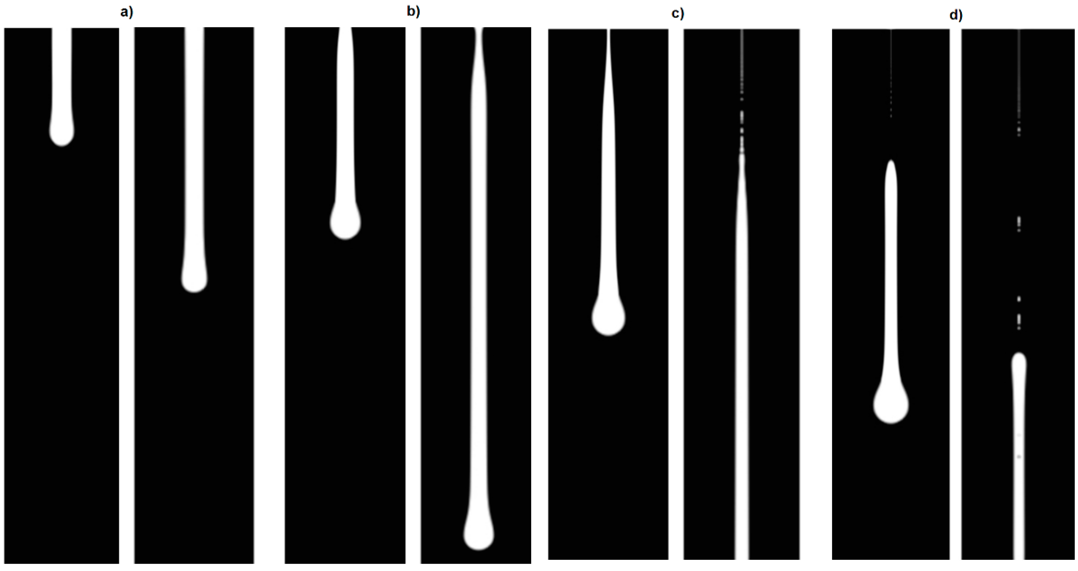
To analyse the influence of surface tension, two cases were selected using 35 (left view) and 73.5 (right view) dyn/cm and keeping all the other operational conditions the same. Figure 3 displays the comparison between cases at four distinct time steps.

For the first two-time steps, the results are fairly similar to those of the case with the lower surface tension progressing faster along the air column. At 18 μs, the drop with the highest surface tension breaks from the nozzle exit, while the drop with the lowest surface tension is slightly behind. Finally, at 24 μs, both drops have broken from the nozzle exit with the case with 35 dyn/cm presenting a long liquid thread, while the case with 73.5 dyn/cm quickly merges into a sphere.

These were predictable results because surface tension is known to contribute to the pinch-off of drops at the nozzle exit [3,27]. Surface tension has an important role in the formation of primary drop and the following satellite(s) because of its dominant effect over the volume force.

4.2. Viscosity

In addition to surface tension, viscosity is also a critical liquid property that affects drop formation. Instead of keeping the liquid inside an elastic membrane, the role of viscosity (and inertia) is to resist the deformation of liquid jet [28]. Common viscosity values found in inkjet printing range from 1 cP (mPas) for pure water to 100 cP [29].

Similarly to the previous case, to analyse the influence of viscosity, two cases were selected using 1 (right view) and 10 (left view) cP and keeping all the other operational conditions the same. Figure 4 displays the comparison between the cases at four distinct time steps.

The case with the lowest viscosity value presents a much more pronounced necking even at 6 μs, leading to a faster breakup time. What really draws attention is that after 24 μs, the liquid thread of the least viscous case presents several necks in different regions, which leads us to believe it will develop into multiple drops with comparable size or at least several satellites.

Overall comparable results in the literature display the same trends, with higher viscosity cases presenting longer tails, and usually requiring more time to form a satellite droplet [30].

4.3. Nozzle Diameter

Besides fluid properties, geometry can have a major influence on the droplet formation process, with the nozzle diameter being the most influential. The printing quality is directly related to the size of the droplet, which in turn is directly related to the diameter of the print-head nozzle. Nozzle diameter can vary greatly depending on the specific application, but is usually of the order of tens of microns.

Similarly to the above studies, to investigate the influence of nozzle diameter in droplet generation and the breakup process, three different diameters were chosen. Figure 5 displays the comparison between two cases at four distinct time steps.

The difference in nozzle diameter is made very clear in the above figure. After 24 μs, in the case with 10 μm in diameter, the droplet already broke from the nozzle exit, while the case with 30 μm is nowhere near breakup. Researchers believe this has to do with the fact that larger nozzle diameters lead to larger dissipation kinetic energy [31]. As the Reynolds number is lower for the case with a smaller diameter, boundary layer effects are expected to be stronger. However, because the average flow rate is the same, the velocity in the center of the jet is larger, leading to the faster dropping dynamics.

4.4. Inlet Velocity

The remaining category is the driving waveform. Within this category, there are a couple of relevant parameters, such as wave shape, frequency, and amplitude. To prevent this study from becoming excessively complex, we have decided to keep the actuation wave curve as it was presented in Section 2, only changing the wave’s amplitude.

Figure 6 displays the ink contours at four time steps for two cases with different velocities, namely at 2.5 and 5 m/s.

In the case of lower velocity, the liquid thread advances more slowly inside the air chamber and also takes longer to break up from the nozzle. On the other hand, higher velocities lead to thinner liquid ligaments and these ligaments collapse into several satellite drops. This is also consistent with the current literature [10,11,13]. The selected range of values agrees with those most used across the literature, with the above-mentioned works being good examples [10,11,13]. When the velocity is reduced to values below this range, the jetting become less repeatable and requires more powerful actuation pulses. Therefore, the study of lower inlet velocities is not so common.

5. Design of Experiments

In the present work, viscosity, surface tension, nozzle diameter, and inlet velocity will act as quantitative or numerical factors. These four factors will be combined under the framework of a face centred design with 25 runs. The face centred design shows the different combinations of levels across the selected factors, as depicted in

Table 3. Face centred design with corresponding factors and ranges.

Run	Inputs
	Viscosity (cP)	Surface Tension (dyn/cm)	Nozzle Diameter (micro)	Inlet Velocity (m/s)
1	10	35	10	2.5
2	5.5	54.25	20	5
3	1	35	30	5
4	10	73.5	30	2.5
5	5.5	35	20	3.75
6	5.5	54.25	30	3.75
7	1	54.25	20	3.75
8	1	73.5	30	2.5
9	1	73.5	10	5
10	10	73.5	30	5
11	1	73.5	10	2.5
12	10	35	30	2.5
13	5.5	54.25	10	3.75
14	1	73.5	30	5
15	10	35	30	5
16	5.5	54.25	20	2.5
17	5.5	54.25	20	3.75
18	1	35	30	2.5
19	10	73.5	10	5
20	10	35	10	5
21	10	73.5	10	2.5
22	10	54.25	20	3.75
23	1	35	10	2.5
24	1	35	10	5
25	5.5	73.5	20	3.75

.

5.1. Empirical Model Validation

One of the main purposes of the design of experiments methodology is to generate an empirical model that is able to predict the responses of interest within the design space. The empirical model can be developed using several mathematical functions, but the most used solution relies on the polynomial fitting. To do so, measures such as $R^2$, $R_{adj}^2$, and $R_{pred}^2$ are extremely useful. The $R^2$ measures how well the model is able to correctly fit the experimental data or the computer-based simulations, as in the present case. The $R^2$ value can sometimes be misleading, causing overfitting of the data. The $R_{adj}^2$ counteracts this overfitting, giving a more reliable tool to evaluate the data fitting quality. The $R_{pred}^2$ measures how well the model is able to re-fit the data when one point is missing. In the present case, all the R measures were close enough between them and to 1, and a high quality fit is expected.

The polynomial degree is found including only the terms, which are able to explain variation beyond what is already accounted for. At these circumstances and after some statistical analysis (sequential model sum of squares and analysis of variance (ANOVA)), the right order model is selected. In this case, the model is quadratic and includes the quadratic, linear, and interaction terms (AB, BC, etc.). Runs based on computer simulations will always provide the same solution and the concept of replicates becomes meaningless. Under these circumstances, the use of some statistical measures such as lack of fit does not bring any data of interest for analysis purposes. From ANOVA, the degree of significance, considering the selected factors, is as follows:

Viscosity > Nozzle Diameter > Inlet Velocity > Surface Tension

These factors were selected because, as was seen in the previous chapter, they have a major influence on the drop formation process.

The final empirical model to predict the break-up time, shown in terms of factual factors, is as follows:

Break-up time = −1.19 × 10⁻⁶ + 5.43 × 10⁻⁷ * Viscosity − 7.72 × 10⁻⁸ * Surface Tension + 1.36 × 10⁻⁶ * Nozzle Diameter − 2.79 × 10⁻⁶ * Inlet Velocity − 5.24 × 10⁻⁸ * Viscosity * Surface Tension + 3.08 × 10⁻⁷ * Viscosity * Nozzle Diameter − 7.54 * Viscosity * Inlet Velocity − 2.16 × 10⁻⁸ * Surface Tension * Nozzle Diameter − 1.78 × 10⁻⁷ * Surface Tension * Inlet Velocity − 3.55 × 10⁻⁷ + Nozzle diameter * Inlet Velocity + 2.10 × 10⁻⁷ * Viscosity² + 1.12 × 10⁻⁸ * (Surface Tension)² + 2.94 × 10⁻⁸ * (Nozzle Diameter)² + 2.59 × 10⁻⁶ * (Inlet Velocity)²

In terms of actual factors, the equation can be used to make predictions about the response for given levels of each factor. Here, the levels should be specified in the original units for each factor. This equation should not be used to determine the relative impact of each factor because the coefficients are scaled to accommodate the units of each factor and the intercept is not at the centre of the design space.

The above equation could be shortened using less significant parameters (p > 0.1). However, at this stage, and because it is important to show how the parameters could relate to themselves, all terms were shown. Further optimization procedures will be carried out using only the significant terms by employing a backward reduction algorithm.

The last step to conclude on the model adequacy is to diagnose the residual for abnormalities. Basically, differences (residues) between experimental data and the computed model are analyzed to verify if the residuals are pure noise or if there are other reasons behind the residuals’ patterns. Figure 7 depicts the normal probability as a function of internal studentized residuals. As can be seen from Figure 7, residuals follow a normal distribution reasonably well, confirming that they are in fact pure noise.

The same procedure was followed considering the break-up length. Minor deviations from normality and constancy of variance were found, which indicates that the developed empirical models are suitable to describe the behaviour of the corresponding responses in the experimental design space.

5.2. Single Response Optimization

Having separately analysed the main parameter categories that influence droplet generation, it is imperative to study how the combination between these parameters actually affect the process.

According to Zhang et al. [32], there are several responses that may affect a well-defined jetting. From their work, it was possible to see that depending on the break-up length and time, droplet-impingement printing and well-defined jet may occur. In this study, the break-up time and length were selected as responses.

Figure 8 and Figure 9 show the response contour plots of break-up time and length after running an optimization algorithm for a single response.

From the studied parameters, nozzle diameter and viscosity appear to have the strongest influence on the chosen responses, with viscosity having a slightly stronger influence between the two, as verified in the construction of the empirical model and corroborated by ANOVA.

Whenever the contour plots tend to a higher ridge, drop pinch-off becomes harder to achieve, thus entering into a non-jettability zone. Interestingly enough, in most cases, this region does not depend on a particular parameter, but rather on the conjunction of several parameters. RSM is the best methodology to identify interactions between several input factors, as well as how their combination affects the main responses of interest. This also shows the crucial role of carrying out response optimization in order to have deeper information on the overall process. With such information, we can define working ranges to prevent operating zones where the drop detachment is just impossible. Regarding the studied responses, most of what was said in the previous chapter still stands.

5.3. Multi-Stage Optimization

The previous analysis was performed while considering a single response. However, inkjet printing, as any industrial process, implies the combination of several restrictions and multiple goals. To be able to perform such an optimization, it is necessary to combine all the goals into a unique function, the so-called desirability function:

$$D={\left({\displaystyle \prod }_{i=1}^n{d}_i\right)}^{\frac{1}{n}}$$

(5)

where $d_i$ is the desirability of each response and $D$ is the overall desirability. $D$ ranges from 0 to 1 (1 being the most desirable condition). After condensing all responses into one global function, it is now important to define which restriction should be applied to each one of the responses (maximize, minimize, bounded between certain values, or even equal to a fixed value).

Two single responses were primarily considered, namely the break-up time and break-up length. From the literature, there are some non-dimensional numbers that characterize the jettability process, namely the dimensionless number Z and the space formed by the Weber and Capillary numbers. These numbers can be defined (respectively) as follows:

$$Z=\frac{\sqrt{inertial force\times surface tension}}{viscous force}=\frac{\sqrt{\sigma \rho d}}{\eta }$$

(6)

$$Ca=\frac{viscous force}{surface tension}=\frac{\eta v}{\sigma }$$

(7)

$$We=\frac{inertial force}{surface tension}=\frac{\rho v^{2}d}{\sigma }$$

(8)

where $\eta$, $\rho$, and $\sigma$ are the viscosity, density, and surface tension of the ink, respectively; and $v$ and $d$ are the droplet velocity and the nozzle diameter, respectively.

Many authors [11,12,13,14] use the Z number as the only index to evaluate the process jettability. However, the Z number presents a major limitation involving all the force terms that are important to droplet generation (inertial, viscous, and surface tension), meaning that several input factor combinations could lead to the same Z value. To overcome such a limitation, Nallan et al. [11] suggested implementing a map of the We−Ca space within which a printability region can be traced. To better understand the usefulness of the We−Re space, Figure 10, Figure 11 and Figure 12 show the Z number, break-up time, and break-up length as a function of the We–Ca space, respectively (computed from the 25 runs of the face centred design).

The We–Ca map brings considerable advantages, such as normalizing the minimal effect of the surface tension force, highlighting the impact of the viscous and inertial forces, and comparing the jettability across ink systems [33]. From the literature, and as mentioned previously in the introduction section, the jettability range regarding the Z number was found to be bounded in the following limits in different works:

−1 < Z < 10

−4 < Z < 14

−0.67 < Z < 50

Kim et al. [34] generated a printability window in a We–Ca space spanning 0 < Ca <4 and 1.5 < We < 15.

Indeed, these can be major restrictions to find the jettability and printability window in our work. Thus, the idea is now to define which of the input conditions (viscosity, surface tension, nozzle diameter, and inlet velocity) are within these restrictions and generate higher/lower/bounded break-up times and lengths. To do so, the desirability function will be implemented, considering the break-up time and break-up length as responses, as well as including the Z number and the We–Ca space as pseudo-responses, in order to constrict the operation window.

Table 4. Multi-optimization using jettability and printability restrictions.

Restrictions	Input Factors				Break-Up Time (s)	Break-Up Length (m)
	Viscosity (cP)	Surface Tension (dyn/cm)	Nozzle Diameter (micro)	Inlet Velocity (m/s)
Z (1–10) Ca (0–4) We (1.5–15) Responses minimization	9.8	53.6	23.2	3.5	1.14 × 10−4	3.35 × 10−5
Z (4–14) Ca (0–4) We (1.5–15) Responses minimization	9.3	65.5	21.4	3.8	1.11 × 10−4	2.18 × 10−5
Z (0.67–50) Ca (0–4) We (1.5–15) Responses minimization	6.1	63.4	23.7	5	1.05 × 10−5	1.61 × 10−5

depicts the optimal operating condition inside the jettability and printability window that minimizes the break-up time and length. From Table 4, the input factors are determined to obtain the required pre-requisites. Using this approach, one can easily ensure a jettability and printability window that identifies where the drops get an easy or hard detachment. This allows for adjusting the input factors for the most proper conditions in any situation.

This methodology presents clear advantages to develop new inks, in order to determine the best inorganic contents to use as an additive or even for design purposes. Using dimensionless numbers as pseudo-responses, additional advantages arise because of the fact that all the considered restrictions and responses are directly related to the input factors. From Table 4, one can clearly identify the intrinsic relation between break-up time and break-up length.

6. Conclusions

Inkjet printing technology was extensively researched in the early 1950s, and is now the most common used technology in printers ranging from small personal consumer models to industrial machines. DoD inkjet holds the majority of the overall market because of its simplicity and feasibility of the miniature system.

Because of its micro scale (both in length and in time scale), experiments are difficult to perform and expensive to replicate. Advances in computational power have allowed researchers to utilize numerical tools to simulate the droplet generation process in a timely, as well as (almost) inexpensive, fashion. Still, there is a clear lack of current literature on the necessary process optimization guidelines to organize all the influential parameters and how their interaction can be optimized to ensure the optimal printability conditions.

A first attempt was made in this article by combining advanced statistical methods (specifically, the response surface method) with the VOF model under the ANSYS^® Fluent framework. A grid independence study was carried out in order to ensure sufficiently accurate results. All the parameters were independently studied to provide an adequate understanding of their influence on the drop formation process.

A single response optimization was conducted to highlight the relative influence of chosen factors in break-up time and length. The results showed that both viscosity and nozzle diameter had the strongest influence on the studied responses.

A multi-stage optimization using several dimensionless numbers that characterize the process jettability was carried out. From the conducted experiments, we were able to minimize the studied responses while using restrictions on these numbers.

The work proved the capability of combining RSM with CFD to decrease experimental procedures while enabling process optimization.