
Surface Runoff in Watershed Modeling—Turbulent or Laminar Flows?


Hydrologic Sciences and Biological & Agricultural Engineering, UC Davis, Davis, CA 95616, USA
Hydrology 2016, 3(2), 18; https://doi.org/10.3390/hydrology3020018
Submission received: 5 April 2016
/
Revised: 20 April 2016
/
Accepted: 25 April 2016
/
Published: 4 May 2016
(This article belongs to the Special Issue Rainfall Simulators as a tool in Soil Science, Geomorphology and Hydrology research and teaching)
Abstract
:Determination of overland sheet flow depths, velocities and celerities across the hillslope in watershed modeling is important towards estimation of surface storage, travel times to streams and soil detachment rates. It requires careful characterization of the flow processes. Similarly, determination of the temporal variation of hillslope-riparian-stream hydrologic connectivity requires estimation of the shallow subsurface soil hydraulic conductivity and soil-water retention (i.e., drainable porosities) parameters. Field rainfall and runoff simulation studies provide considerable information and insight into these processes; in particular, that sheet flows are likely laminar and that shallow hydraulic conductivities and storage can be determined from the plot studies. Here, using a 1 m by 2 m long runoff simulation flume, we found that for overland flow rates per unit width of roughly 30–60 mm2/s and bedslopes of 10%–66% with varying sand roughness depths that all flow depths were predicted by laminar flow equations alone and that equivalent Manning’s n values were depth dependent and quite small relative to those used in watershed modeling studies. Even for overland flow rates greater than those typically measured or modeled and using Manning’s n values of 0.30–0.35, often assumed in physical watershed model applications for relatively smooth surface conditions, the laminar flow velocities were 4–5 times greater, while the laminar flow depths were 4–5 times smaller. This observation suggests that travel times, surface storage volumes and surface shear stresses associated with erosion across the landscape would be poorly predicted using turbulent flow assumptions. Filling the flume with fine sand and conducting runoff studies, we were unable to produce sheet flow, but found that subsurface flows were onflow rate, soil depth and slope dependent and drainable porosities were only soil depth and slope dependent. Moreover, both the sand hydraulic conductivity and drainable porosities could be readily determined from measured capillary pressure displacement pressure head and assumption of pore-size distributions (i.e., Brooks-Corey lambda values of 2–3).
1. Introduction
Modeling the process of overland (sheet) flow generation from forested catchment slopes remains compromised as the threshold combination of soil hydraulic properties, slope, surface conditions (e.g., roughness, microtopography) and onflow (rain or snowmelt) rates that determine whether flows remain subsurface or break the surface are unknown [1,2]. That is, what combination of conditions (e.g., slope, onflow rate and soil hydraulic conductivity) results in infiltration excess (Hortonian) or saturation excess (Dunne) overland flows? Clarification of this distinction is critical towards assessing subsurface-surface hydrologic connectivity [3] within the watershed as well as estimation of flow travel times to streams and the surface shear stresses (overland flow velocities, or stream power) associated with erosion rates. Field observations from hundreds of rainfall/runoff simulations and during storm events in the northern Sierra Nevada and coastal CA watersheds have indicated that when near surface soils are unsaturated, overland flow generation only occurs on compacted soils (e.g., roads and landings) and only occasionally from less disturbed or restored forest soils [4,5,6,7,8,9]. In the less disturbed or restored soils, rainfall (even at rainfall rates of 100 mm/h) or snowmelt surface onflows (e.g., [10]) become subsurface interflows that may appear as seeps downslope at low gradient areas, creek banks, or roadside ditches. In contrast, on compacted soils such high rainfall rates result in overland flow within a few minutes and even after 20–60 min of 60–100 mm/h rainfall, soil wetting depths can be ~10 mm suggesting an arbitrarily thin saturated surface soil layer that is forcing runoff to develop. Various watershed models recognize this thin layer (e.g., [11,12]) and assign an arbitrary layer thickness as a transition between the equations representing surface and subsurface water flows. Similarly, most if not all, watershed modeling efforts (e.g., [13]) presume that overland flows occur under turbulent conditions and employ the associated frictional loss Manning’s equation to describe such flows, though from both modeling and field observations, it appears that hillslope overland sheet flow conditions are typically laminar with flow depths on the order of 1 mm [14]. As hillslope overland flows control multiple aspects of several important watershed processes including rill development [15], sediment and pollutant dispersion [16] and travel times [17], properly characterizing the overland sheet flow conditions is critical. For example, estimation of flow travel times, erosion shear stresses and possible erosion rates along hillslopes all depend on correctly determining the overland flow velocity, which depends on whether the flow is assumed to be laminar or turbulent; thus, incorrectly calculating these velocities may be part of the inability of watershed models to predict or capture the rapid, or “flashy” hydrologic response of mountain watersheds to runoff (rain or snow) events (e.g., [18]).
1.1. Experience with Tahoe Rainfall & Runoff Simulations
When overland flow is generated by infiltration or saturation excess even at runoff rates likely exceeding those occurring naturally, it is generally assumed to occur as turbulent flow, though it appears that it may be better represented by laminar flow conditions. Considering rainfall-runoff simulations in the Lake Tahoe Basin and elsewhere [6,7,8,9] across a range of slopes (5%–80%) of disturbed and less-disturbed forest soils indicated that at rainfall rates ranging from 60 to 180 mm/h, steady infiltration rates averaged more than 60 mm/h while runoff rates rarely reached 45 mm/h and in many cases, there was no runoff at all after more than 40 min of high intensity rainfall. That is, in field rainfall simulation studies, there were replicate plots that did not produce runoff while adjacent plots did for the same rainfall rates, soils and apparent surface conditions, suggesting that a threshold of combination of parameters exists that result in surface runoff, hydrophobicity notwithstanding. When high rainfall rates were necessary [7] to initiate runoff, in many cases they all exceeded durations of such high intensity natural rainfall, or far exceeded typical snowmelt rates in the basin. Thus, on a typical 50% roadcut slope, a simulated rainfall induced runoff rate of 25 mm/h (equivalent to a surface flow per unit width of 5.6 mm2/s) implies average flow depths of less than 0.1 mm under both turbulent and laminar flow assumptions, respectively, or Reynolds numbers less than one. Similarly, results from a 1-m wide runoff simulator on a similar slope of nearly 52%, but at a much greater onflow rate of 3.4 Lpm for an average surface flow per unit width hundred times greater of 57 mm2/s results in a proportionately greater Reynolds number of 52 for laminar flow, while for turbulent flow it remains far smaller than one. In addition, from a runoff modeling perspective in the Tahoe Basin (e.g., Homewood Creek watershed, [6]), during a wet-year calibrated simulation, the maximum daily runoff value was about 19 mm during a spring rain on snowmelt day. The 19 mm runoff across the approximately square mile basin occurred within about a 10-hour period such that the average runoff rate was at most 2 mm/h implying an areal average Reynolds number of <0.1. This ~2 mm/h snowmelt rate is roughly consistent with, though smaller than rates of ~5 mm/h measured using artificial rain on snow events at Soda Springs just outside of the Tahoe Basin by [19]; however, the measured snowmelt rates are still well below those from rainfall simulations noted above. In the integrated physical modeling conducted by [1] in both a relatively steep forested watershed of Oregon and the mildly sloping rangeland Oklahoma watershed [20], overland flow depths outside of concentrated flow channels were of similar magnitudes, typically on the order of 0.1–1 mm. While these modeling flow depth estimates depend in part on use of the Manning’s equation, when combined with observations from rainfall/runoff simulations, they underscore the concept that overland flow rates are such that Reynolds numbers are at least an order of magnitude below the value of 500 often assumed to differentiate laminar from turbulent overland flow. While at relatively small slope gradients of <10%, the difference in predicted flow depths and velocities using either laminar or turbulent (Manning’s) flow equations are relatively minor, use of Manning’s equation still requires assumption of a flow-depth dependent roughness value ‘n’ in watershed modeling efforts. At the much greater slopes commonly encountered (10%–100%) in forest watersheds, use of Manning’s equation may result in over-estimation of the shallow flow depths and under-estimation of average velocities that in turn affect estimated flow travel times and the shear stresses associated with sediment detachment and-transport rates (erosion).
In addition to better understanding when and how overland flow occurs, improved understanding of the hillslope soil hydraulic properties following soils restoration directed at improving infiltration capacities and soil hydraulic function is key towards determining shallow interflow rates and storage capacities that influence hillslope ‘connectivity’ to riparian zones. Jensco and McGlynn [3] assert that “We should no longer rely on statistical criterion to determine when and where we sample, but be better guided by experimental criteria. One possible way to do so is to investigate how storage of water occurs in different catchments and how these stores fill up (or down) and link (or not) to produce (dis)connected flow.” Jensco and McGlynn [3] use the term to describe the initiation of a shallow groundwater table across hillslope, riparian, and stream zones [21,22,23]. Development of water table connectivity across the hillslope-riparian-stream continuum may be considered a requisite for throughflow or interflow [21,24] and solute transport to streams [23,25,26,27]. In mountainous catchments, there are often strong relationships between landscape topography and runoff generation [28,29,30,31,32], spatial sources of runoff [24,33], and water residence times [34,35,36]. Jencso et al. [21] proposed the topographic metric of the upslope accumulated area (UAA), the amount of land draining to a point in the landscape. Many of the formative hillslope hydrology studies [28,29,37,38] observed increased subsurface water accumulation in topographically convergent hillslope areas and in greater UAAs. Aside from climate factors (e.g., rainfall intensity and snowmelt rates), it appears that the primary controlling factors for both surface and subsurface hydrologic connectivity are soil depths, flow path distances and gradients to the creek, accumulated drainage area above the node (e.g., UAA) and available drainable porosity associated with slope and soil depth [39].
1.2. Research Hypotheses and Objectives
This project originated from an effort to relate observed field simulated runoff rates from Rainfall [40] and Runoff Simulators to model-predicted values so as to better infer soil properties associated with hillslope soils restoration efforts and estimation of watershed sediment loading rates [5]. Such modeling effort was hampered by the inability to a priori predict when surface runoff generation would result from infiltration excess, rather than saturation excess (more readily simulated when available soil water storage is filled). This inability stems from lack of definition of surface factors such as hydrophobicity and the near surface saturated soil layer thickness controlling infiltration rates that could not be independently determined and depended on whether rainfall or runoff simulator field methods were employed. Moreover, as the initiation and duration of overland flows often depends on levels of antecedent soil moisture, some assessment of soil drainage rates in the field may be needed at the hillslope scale. We add this observation to what Jensco et al. [21] and others have underscored, i.e., that the relative thickness, drainable porosity and slope of the shallow soil-interflow layer (0.05–2.0 m depths) is critical towards development of subsurface and surface water connectivity within the watershed. The effort to reconcile predicted and observed surface/subsurface flow rates as well as the need to determine when or whether surface flows originated from excess rainfall or saturation overflow so as to better link erosion rates to the driving shear forces led to two overarching project hypotheses; (1) that infiltration excess overland flow is more readily generated at high slope gradients (>20%) as compared to low (<10%), and (2) that infiltration or saturation excess shallow overland flows at observed or simulated runoff rates were laminar rather than turbulent at field slopes of 5%–80%. The related research objectives included;
- (a)
- determination of flow depths and Reynolds (Re) numbers for a range of slopes and flow rates and planar surface roughness conditions,
- (b)
- determination of fine-sand surface runoff, interflow and drainage rates for the range of slopes and flow rates considered in (a) in an effort to determine the combination of slope and onflow rates required to generate infiltration excess overland flow, and
- (c)
- development of a simple hillslope runoff-interflow model that includes basic soil hydraulic properties (effective conductivity and drainable porosities or yields) readily assessed in the field.
This paper considers project objectives (a) and (b), while objective (c) will be addressed in a separate publication.
2. Experimental Methods
2.1. Theory—Laminar & Turbulent Overland Flow Equations
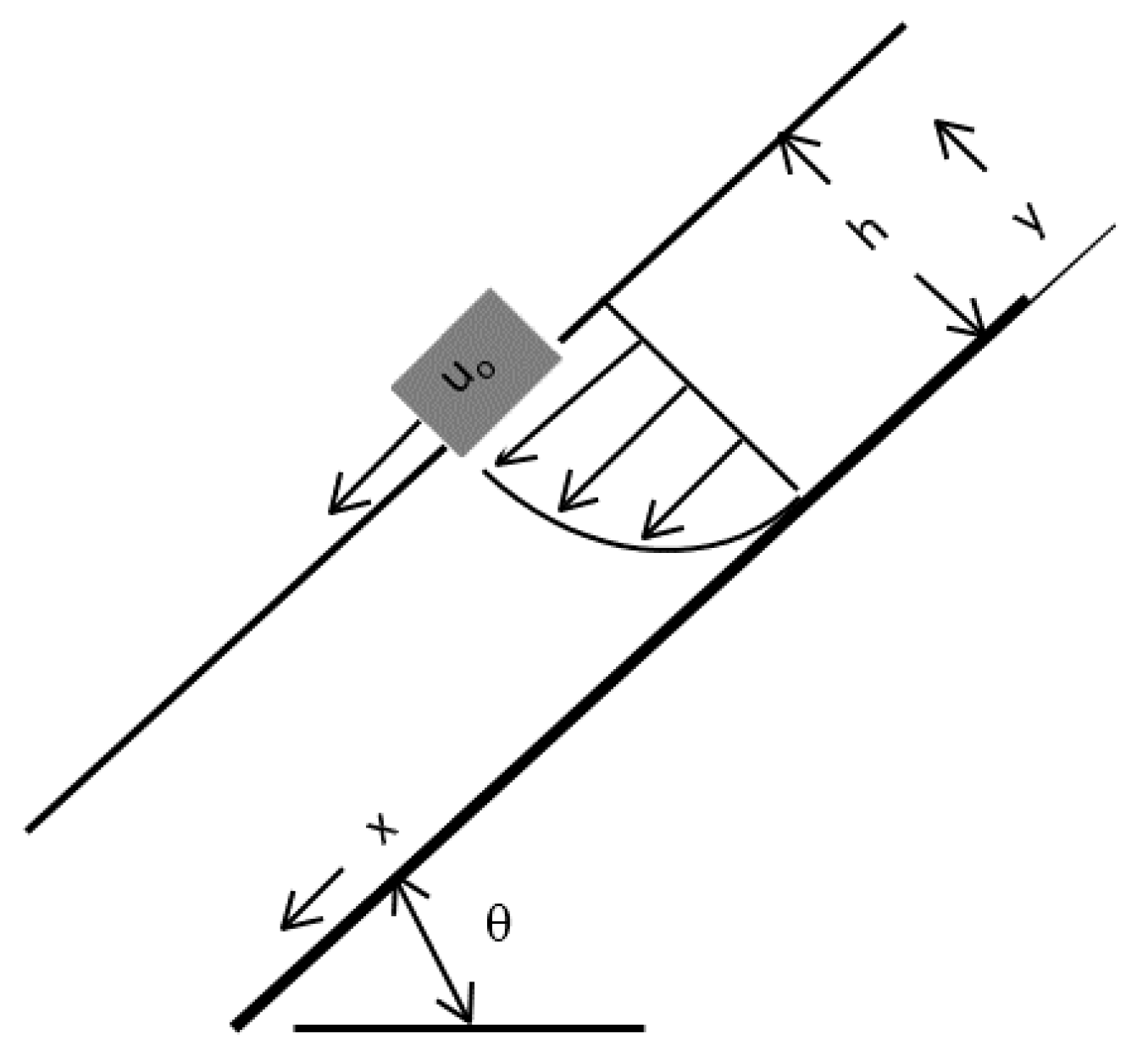
Most watershed modeling efforts and associated estimation of erosion rates assume turbulent flow conditions and employ the well-known Manning’s equation to relate overland or channel flow rates to flow depth, velocity and hillslope, or channel gradient. Of course, use of Manning’s equation implies that an appropriate surface roughness value ‘n’ can be identified. While originally developed and understood to apply at slopes less than about 10%, Manning’s equation is presumed to apply at much greater slopes as well in watershed modeling. In contrast, the general derivation of the laminar flow equation for thin films on inclined planes at any angle θ to the horizontal requires only the assumptions of the ‘no-slip’ boundary condition together with constant fluid properties [41]. Considering two-dimensional steady flow as shown in Figure 1, the shear force as given by the fluid viscosity and parabolic velocity function is balanced by the gravitational force (unit weight) on the fluid body in the direction of flow. That is,
where μ is the water viscosity, ρ is the water density, h is the water depth and uo is the maximum velocity such that the mean velocity, um from the parabolic vertical velocity distribution is simply um = (2/3)uo. Then, the total flow rate per unit width, Q, is then given by
where the Reynolds number is determined from Re = Qρ/μ.
2μuo/h = ρgh sin θ
Q = um h = (ρgh3/3μ)sin θ
From Equation (2), under steady laminar flow conditions, it is apparent that surface flow velocity is roughly proportional to the slope rather than the square root of the slope and there is no need to identify the roughness value ‘n’, whereas the laminar mean flow velocity is given by
where the slope approximation replacing the sine function is from the best fit power curve.
um = (ρgh2/3μ)sin θ ≅ (0.7524ρgh2/3μ)S0.983
The familiar Manning’s equation for broad shallow flow of depth ‘h’ takes the form
where S is the slope equivalent in concept to the angle θ in Figure 1. Then, the Manning’s mean flow velocity is given by
Q = (1/n)h1.667S0.5
um = (1/n)h0.667S0.5
Note that in Equation (3), the mean flow velocity is proportional to the flow depth squared and directly to the slope, whereas under turbulent flow assumptions (Equation (5)), the mean velocity is proportional to the flow depth to the 2/3rd power and the square root of the slope. This difference between Equations (3) and (5) also plays out in the formulation of the water storage as a function of depth, or celerity (c = ), as in the kinematic-wave equation often applied in hydrologic modeling [42]. That is,
Thus, laminar flows suggest a much greater influence of slope and water depth on wave celerity than would be suggested by assuming turbulent flows.
2.2. Experimental Apparatus and Measurement Methods
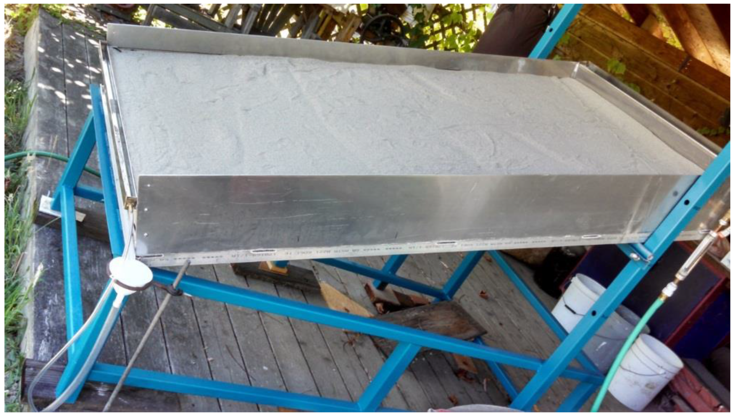
Three sets of experiments were performed to address the basic project objectives outlined above. For research objectives (a) and (b), a tilting aluminum 1 m wide by 2 m long and 0.25 m high ‘sandbox’ was used (see Figure 2). The ‘sandbox’ could be set at slopes ranging from 0% to 75%. Stainless steel troughs with smooth lips were installed at the upper and lower ends of the box to supply or collect water uniformly across the 1 m width of the box. Inlet flow rates were controlled and measured using valves and calibrated in-line flowmeters and outflows were measured directly using flowmeters or graduated cylinders and a stopwatch. Flow depths across the width of the box and approximately 0.7 m from the upper lip were measured after steady flow was established. The water depth was determined using a micrometer with an internal accuracy of ±0.001 mm. The micrometer rod with a truncated cone tip was lowered to the bare aluminum or sandpaper grain surface, set to zero and then retracted until the surface tension broke (~2 mm above the water surface) and then lowered again until just contacting the water surface where the measured depth was recorded. This procedure was repeated 3–5 times at each location until the depths measured were repeated within a range of ±0.005 mm. Flow depths were determined at slopes of 10.7%, 20.6%, 36.6%, 51.8% and 66.2% and a range of onflow rates that included 1.6, 2.25, 2.8 and 3.43 Lpm. To simulate various ‘roughness’ values beyond that of the smooth aluminum, fine to coarse grit (#60, #100 and #150) sandpaper was attached to the aluminum base of the flume box and the flow depths measured as described above. The sandpaper grit sizes used (roughly 100–270 μm) spanned the fine-sand grain size used in the runoff experiments associated with objective (b) above.
In the runoff simulation experiments directed at objective (b), washed Monterey #30 fine sand was placed in the flume box in layers to uniform depths of 71, 143 or 215 mm. The sand surface was rolled smooth using an 80 mm diameter steel pipe prior to initiation of surface flows at rates of 1.6–3.4 Lpm. Here, we consider the runoff and drainage results from the experiments at a sand depth of 143 mm and slopes of 10.7%, 20.6%, 36.6% and 51.8% as the other results were similar. An interchangeable stainless steel screen at the lower end of the box was outfitted with small collection channels that enabled measurement of subsurface flow and drainage rates following termination of surface onflow. A similar collection channel for surface runoff was available, but as will be described later, this channel only collected flow after the sand became relatively saturated.
To determine the soil-water retention and drainage characteristics of the Monterey fine sand used in the sandbox runoff experiments directed at objective (b), simple column tests were developed. Vertical columns constructed of 20 PVC rings (20 mm tall by 50 mm diameter) were used to determine the fine sand water retention and hydraulic conductivity in anticipation of predicting sand-water retention in the flume box at various sand depths and slopes following runoff simulations. The sand was carefully packed into the columns, saturated from the bottom upwards to limit air entrapment and allowed to equilibrate for 24–48 h with a ponded water depth of about 10 mm. After equilibration, the columns were allowed to freely drain from the base and the outflow rates and volumes drained recorded. After drainage practically terminated (~12 h), the sand PVC rings were separated, the wet sand weight recorded, the sand oven-dried and the dry sand weights recorded to determine the water content as a function of height (capillary pressure head) above the column base. Several column experiments were conducted to determine the average sand-water retention function and drainable porosities for the Monterey fine sand.
3. Results and Discussion
3.1. Laminar or Turbulent Sheet Flows, the Distinction Appears to be Important
While it is possible to measure average overland flow rates in the field rainfall and runoff simulations (e.g., [7]), determinations of average flow depths are generally not possible due to the variable surface conditions and small depths; hence the need for the aluminum sandbox to determine if the field shallow flow depths were consistent with laminar or turbulent flow conditions. These results are considered first followed by the fine-sand water retention and drainable porosity measurements, and finally the sandbox runoff experimental results.
Use of the aluminum box enabled control of onflow rates and surface flow conditions, at different slopes (10%–66%), such that flow depths could be measured more precisely than possible in the field. The experiments were designed to address the first research objective and to address the second hypothesis. Table 1 summarizes the results of the flow depth measurements for four different onflow rates and five different slopes. For each onflow rate tested on the bare aluminum surface, a simple wave pattern was established across the 1 m width of the box and an effort was made to measure the wave celerity visually to determine its possible impact on the flow depth measurements. Estimated wave speeds ranged from 170 to 220 mm/s for the 10.7% slope, 210–290 mm/s for the 20.6% slope and 280–350 mm/s for the 36.6% slope and were at even greater speeds for the steeper slopes for the flow rates summarized in Table 1; these speeds were consistent with those derived theoretically as shown in Figure 3. As the flow depth measurements each required several minutes, the high wave speeds suggest that the depth measurements represent something of an average flow depth irrespective of wave height or speed. Generally, as suspected due to the low Reynolds numbers (24–51), the measured flow depths were consistent with those predicted assuming laminar flow from Equation (2) for the smooth (bare) aluminum surface. Similar results were obtained for the sandpaper surface conditions in which the measured flow depths for the fine sandpaper (#150 grit) were the same as those for the bare aluminum. Measured flow depths for the coarser sand paper (#60 grit) were roughly 5% less than those for the bare aluminum, presumably due in part to the flow between adhered sand grains and below the level of the micrometer rod tip. Measured flow depths for the medium sand paper (#100 grit) were slightly less than those for the bare aluminum, but not significantly so. Water surface tension effects were evident and manifested in the difficulty establishing uniform flow across the width of sandbox after the initial fingered flow across the sandpaper. For the bare surface condition, uniform flow across the box width was easily obtained by wiping across the surface with a sponge. A similar approach was used with the sandpaper surfaces using a rag; however, establishing uniform flow across the box width became increasingly difficult as the sandpaper grit size and box slope increased. In fact, only fingered flow occurred, regardless of wiping, at the steepest two slopes for both the #60 and #100 grit sandpaper surfaces, and flow depth measurements were compared with depths determined from approximated flow width areas instead such that flow rates per unit width were greater than those listed in Table 1. Such fingered flow was also evident in field runoff simulations (Hogan, personal communication) as well as in the sandbox runoff experiments.
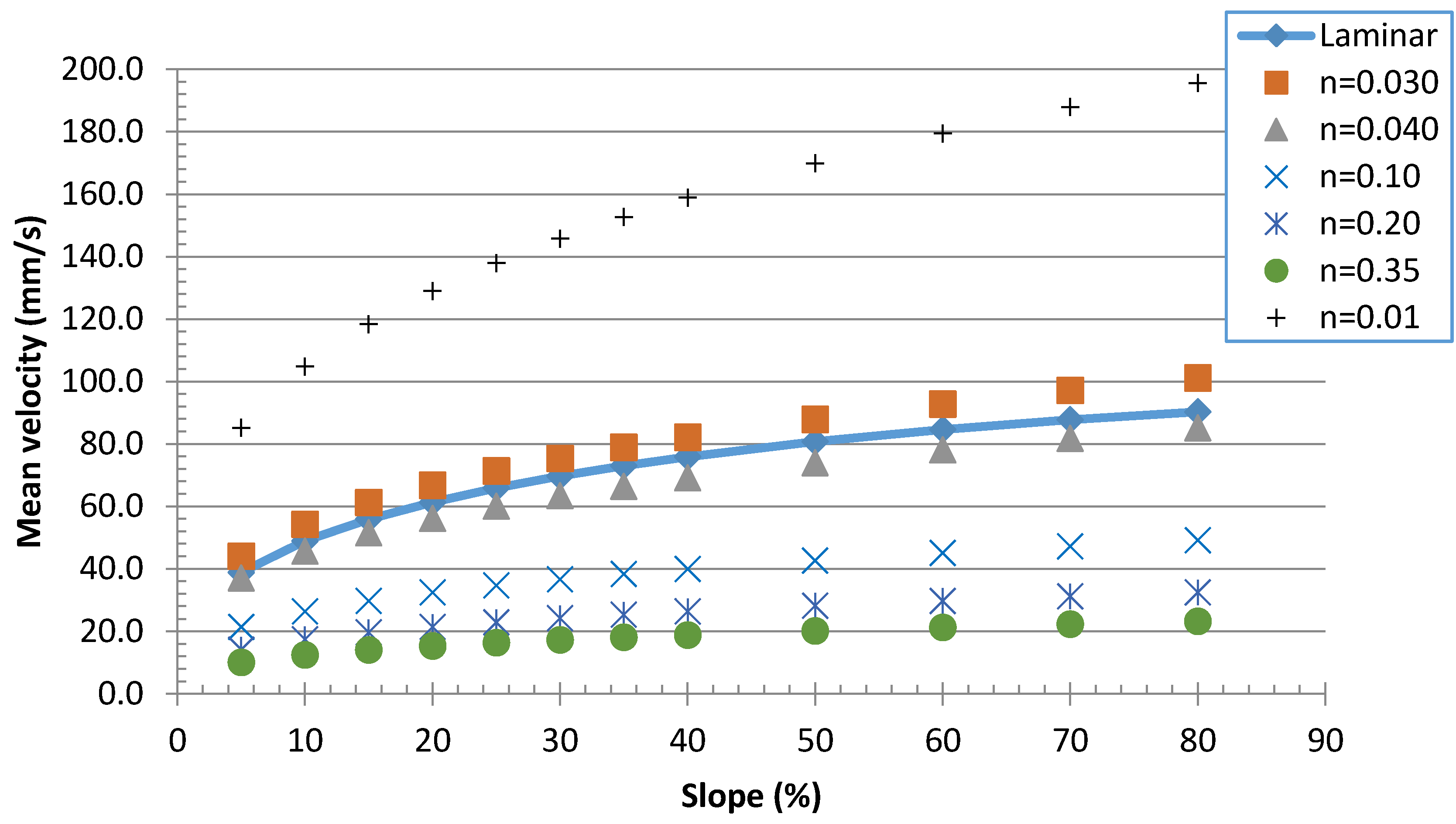
Nonetheless, for all surface conditions considered, measured flow depths were consistent with those predicted by laminar flow assumption embodied in Equation (2), rather than the turbulent flow conditions represented by Equation (3) and used in physical watershed modeling efforts to date. Using the predicted flow depths, the “apparent” Manning’s n values were computed and are listed in the last column of Table 1. Apparent n values decrease with increasing flow depth or flow rate and roughly average 0.025, a value much less than that typically assumed (~0.35) in watershed modeling [43] for relatively “smooth” (e.g., dirt road, grassed, bare uncultivated soil) surfaces. To illustrate how mean velocities determined from Equations (3) and (5) differ, Figure 4 illustrates the dependence of mean velocity on hillslope gradient assuming a typical range of n values and an overland flow rate per unit width of 20 mm2/s at 16 C (equivalent to Re = 18). Note that at slopes less than about 40%, the dependence of mean velocity on slope is practically equivalent between the laminar and turbulent flow conditions, especially for n values between 0.03 and 0.04; however, at larger or very small (e.g., glass n < 0.01) n values, Manning’s equation underestimates, or overestimates, respectively, the velocities by a factor of 2–3 times at any slope. Also shown in Figure 4 and Figure 5, use of an n value of approximately 0.035 in the Manning’s equation at slopes less than ~40% is required to obtain flow depths and mean velocities roughly equivalent to that determined by the laminar flow equation. An even smaller ‘n’ value (~0.02) is required to match turbulent and laminar flow celerities (see Figure 3). The range of surface runoff rates considered and listed in Table 1 readily exceed those commonly found in the field (e.g., Tahoe Basin; [40]), or predicted in rainfall-runoff modeling, suggesting that assumption of laminar flow conditions for all but the defined channel flows are likely more appropriate in hillslope modeling efforts rather than assuming application of the Manning’s equation and guesstimation of ‘appropriate’ roughness ‘n’ values.
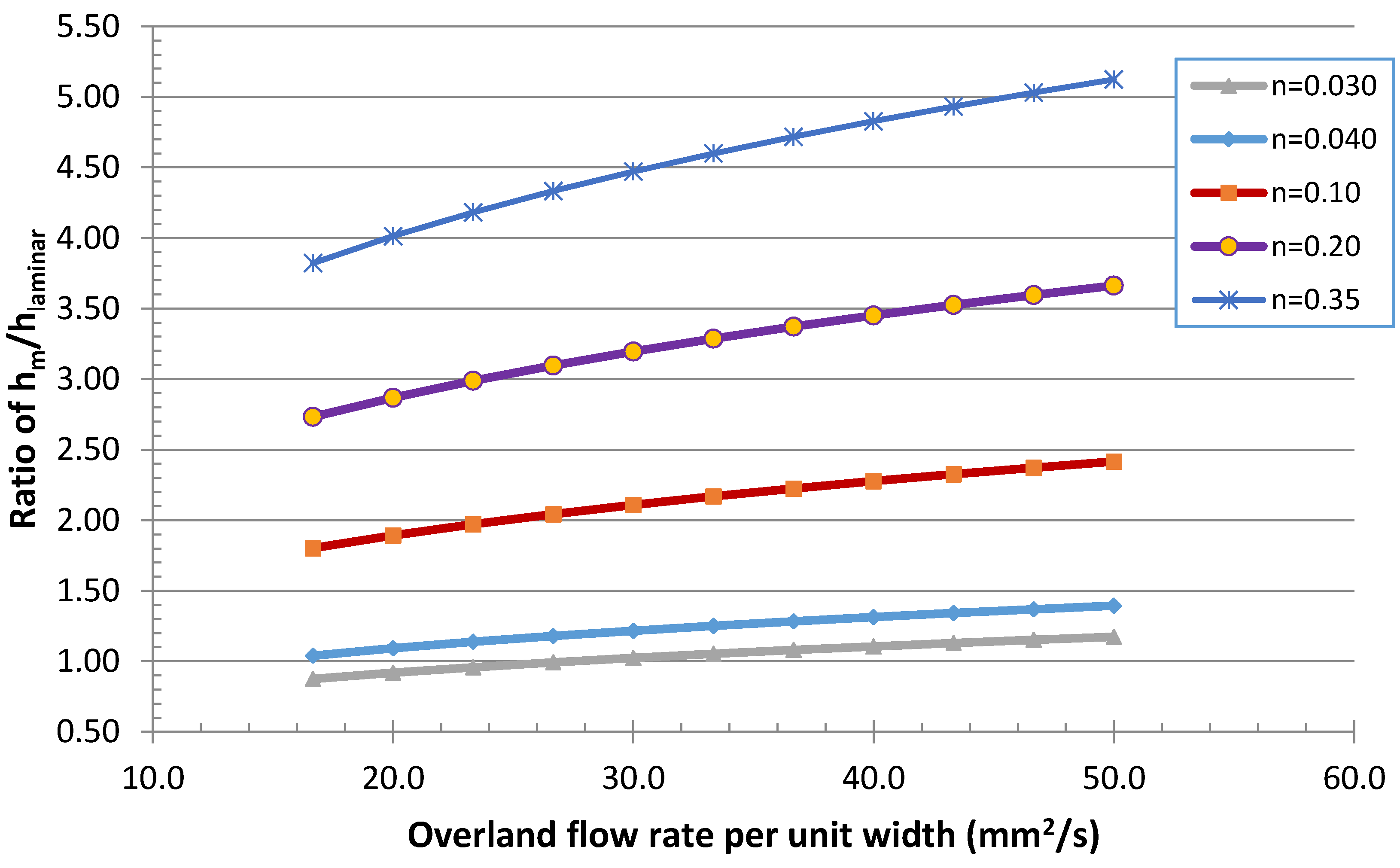
Similarly, anticipating the later discussion of the experimental methods, Figure 5 illustrates the ratio of flow depths determined assuming turbulent and laminar flow conditions, respectively, on a 20% slope at a range of unit width flow rates and ‘n’ values. The overland flow rates shown equate to Reynolds numbers that range from 15 to 45 and corresponding laminar flow depths of 0.31–0.44 mm, respectively. For any given ‘n’ value there is little change in these ratios for the slope range of 5%–80% slopes across the flow rates shown. An equivalent graph of the ratios of turbulent to laminar flow mean velocities would be the same as that shown in Figure 5 for the ratio of depths. This distinction in velocities is important towards estimating stream power associated with soil detachment and definition of “erodibilities” from RS studies where Grismer [40] found that laminar flow-determined mean velocities better represented the dependence of soil detachment on stream power than those from assuming turbulent flow velocities. It is also important to note, that the flow depths associated with n = 0.35 as usually assumed in watershed modeling [20], are 4–5 times greater than those assuming laminar flow, thereby resulting in far greater surface storage of water on the hillslope than would occur under laminar flow assumptions. Combined with predicted mean overland velocities of turbulent flow being about 1/3rd of the value for laminar flow (Figure 2) suggests that the watershed models employing turbulent overland flow assumptions with n = 0.35 will predict much slower stream response times to sheet flows from adjacent hillslopes as well as underestimating surface shear stresses associated with erosion.
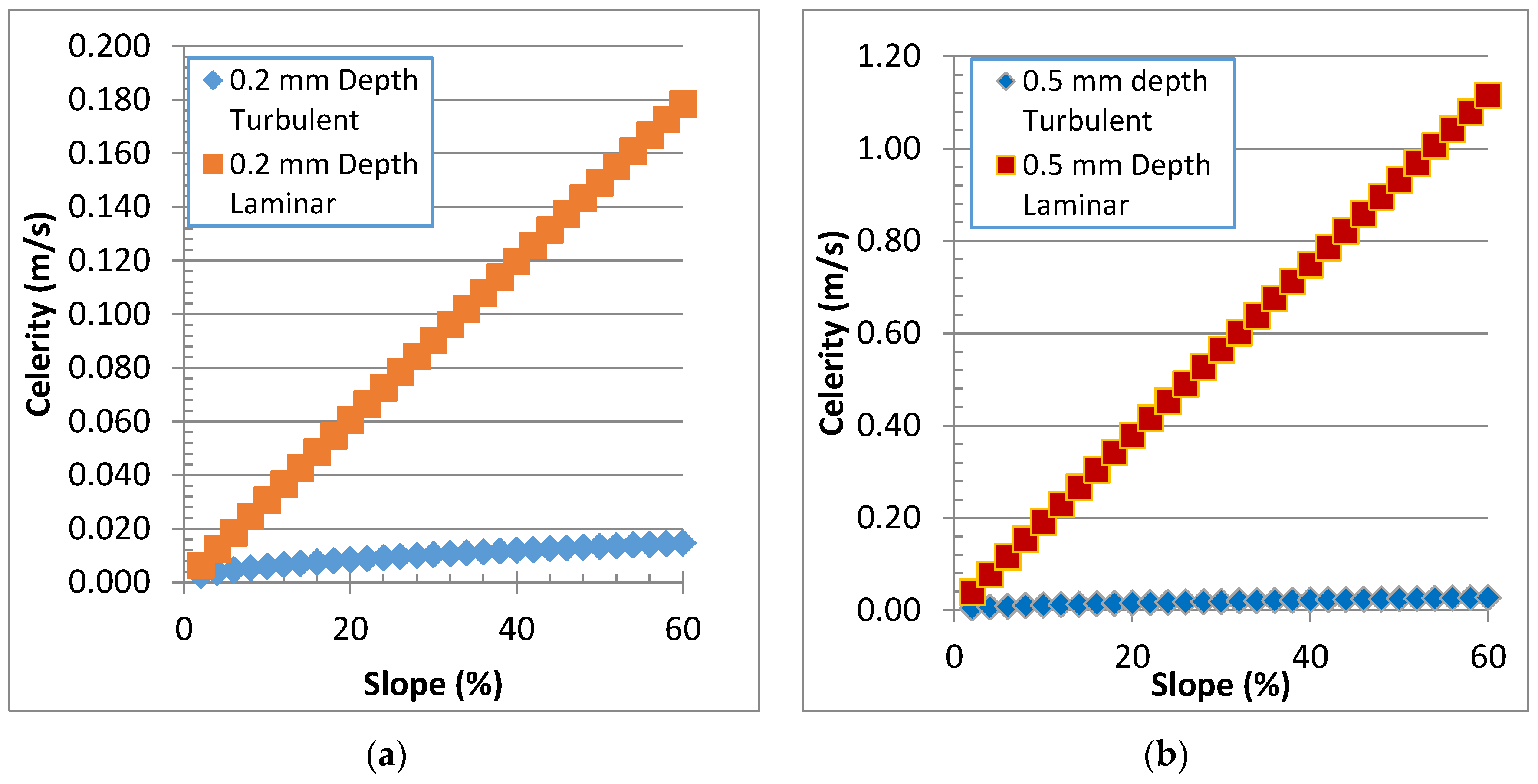
Finally, the distinction in laminar versus turbulent (n = 0.3) flow assumptions is even more apparent with respect to wave celerities used in the kinematic wave modeling of overland sheet flows as shown in Figure 3 for water depths of 0.2 and 0.5 mm. Note that celerities for the 0.2 mm and 0.5 mm depths across the slope range of 0%–60% for turbulent flows range from 3 to 30 mm/s, whereas for laminar flows they range from 6 to 1120 mm/s. To achieve similar celerity values between laminar and turbulent flow assumptions for shallow slopes <10%, the ‘n’ value required is the very small 0.025 as noted above, more than an order of magnitude less than that used in watershed modeling of overland flows (e.g., [20]). As with the differences in flow depths and velocities between turbulent and laminar flow assumptions noted above, the much smaller celerities derived from Manning’s equation would suggest that the turbulent overland flow assumptions will substantially overestimate the time for stream response to hillslope runoff.
3.2. Can Hillslope Drainage be Predicted from Simple Laboratory Measurements?
The fine-sand columns studies and sandbox experiments were designed to complete the second research objective while providing some insight into the first hypothesis considering the thresholds associated with determining when surface runoff results from infiltration excess as compared to saturation excess. The fine sand used for the sandbox runoff experiments was chosen because it had grain sizes between the fine ‘volcanics’ and coarser ‘granitic’ soils encountered in the Lake Tahoe Basin [7]. Table 2 summarizes the water-retention characteristics of the fine sand from the laboratory column experiments. The estimated displacement pressure head was 130 mm with a pore-size distribution index of ~3.4, and the column measured Ks was ~900 mm/h; these values are consistent with other sands [44]. Andesitic and granitic soils in the basin are characterized as sands to loamy sands with relatively high hydraulic conductivity [7]. From RS studies, Grismer [40] measured surface soil effective hydraulic conductivities averaging about 70 mm/h for both soils, while field permeameter-based measurements (bore-hole methods) of saturated hydraulic conductivity, Ks, were about an order of magnitude larger (700–900 mm/h).
In the sandbox runoff experiments, the original presumption of measuring both surface and subsurface runoff was barely realized because for all slopes and sand depths subsurface flow comprised all of the outflows until the sand was completely saturated and began slumping within the sandbox. This repeated observation of much larger effective hydraulic conductivities within the sandbox was somewhat inconsistent with the column-measured fine-sand hydraulic properties described above and listed in Table 2. In the sand column tests, the 0.13 m displacement pressure head suggests a Ks of 1.7 m/h based on pore-size distribution considerations [44]. Despite efforts to pack the sandbox to a similar bulk density as the columns, steady subsurface flows in the sandbox experiments (e.g., onflow rate of 3 Lpm on a 36.6% slope) implied Ks values greater than 5 m/h. This discrepancy was due in part to the lower bulk density of the fine sand that could be achieved in the sandbox (1590 kg/m3) as compared to the laboratory columns (1700 kg/m3), so a second set of column tests were conducted in which the sand was only loosely packed, which resulted in an equivalent pore-size distribution (~3.5) as the original tests, and a slightly greater porosity of 39%, but a smaller displacement pressure head of ~80 mm. The latter implied a Ks of 6.6 m/h based on pore-size distribution considerations for fine sands [40]. This second set of columns resulted in more-or-less the same water contents as listed in Table 2 with the exception that all the water contents were shifted up such that for capillary pressure heads of 100 and 120 mm, for example, the water contents were 0.34 and 0.33, respectively.
Despite the use of large onflow rates and steep slopes in an effort to develop sheet flow across the fine sand, in nearly all of the sandbox experiments with 143 mm deep sand and onflow rates greater than ~2 Lpm (~33 mm2/s), only surface runoff fingers developed on the sand surface; the fingers rarely extended more than 100–200 mm before submerging or branching and always remained behind the average subsurface wetting front. Formation of overland flow appeared to be related to aspects of the microtopography and wettability of the sand as well as, of course, its relatively large hydraulic conductivity. When a surface runoff finger reached the end of the sandbox, subsurface flows were already nearly equivalent to the onflow rate and the sand had destabilized within the box. At the steeper 51.8% sandbox slope, onflow rates less than 2 Lpm did not result in surface fingered flow, though at greater flow rates, incipient seepage faces appeared in the sand prior to the sand slumping in the box. As a result of the limited surface runoff achieved in any of the sandbox experiments, the research focus shifted towards developing the data necessary for the subsurface flow modeling effort of research objective (c) and determination of effective drainable porosities.
While several sandbox runoff experiments were conducted at the three fine-sand depths of 71, 143 and 215 mm, and a variety of slopes, onflow rates and initial soil moisture conditions from dry to uniformly wetted, we chose to focus on the soil moisture conditions more likely to develop in a hillslope between storms; referred to here as the state of ‘natural drainage’. To simulate this ‘natural drainage’ case, the fine sand was saturated, the box slope established and the 143 mm thick sand allowed to drain for 36–48 h (when outflow practically ceased) prior to initiation of a new runoff experiment. The resulting soil moisture distribution in cross-section was then similar to that associated with a hillslope adjacent to a stream having a seepage face of about 100 mm height at the sandbox end screen. That is, the lower portion of the sandbox was at greater moisture contents than the upper portion where the onflow occurred, consistent with the water retention characteristics summarized in Table 2.
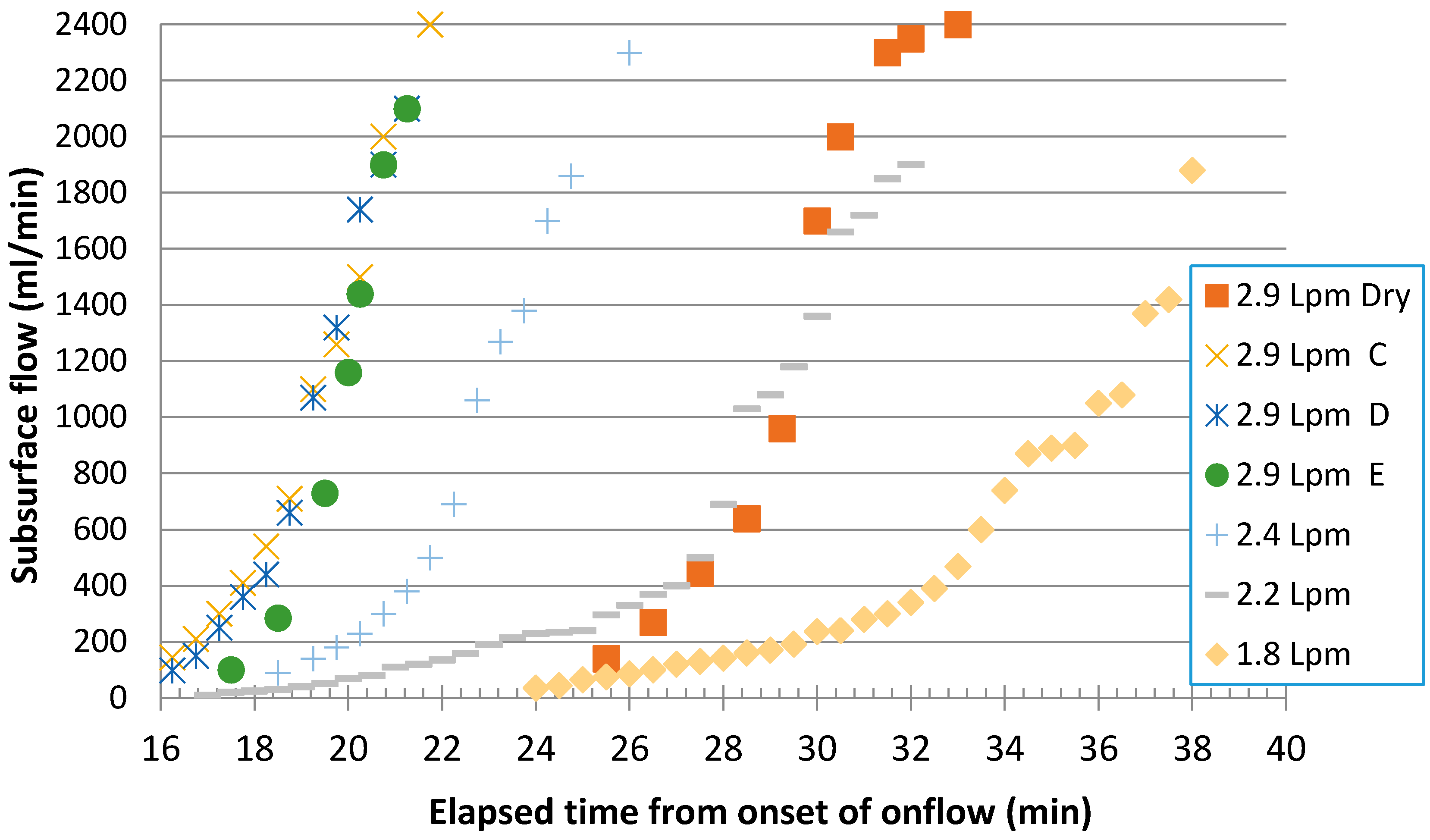
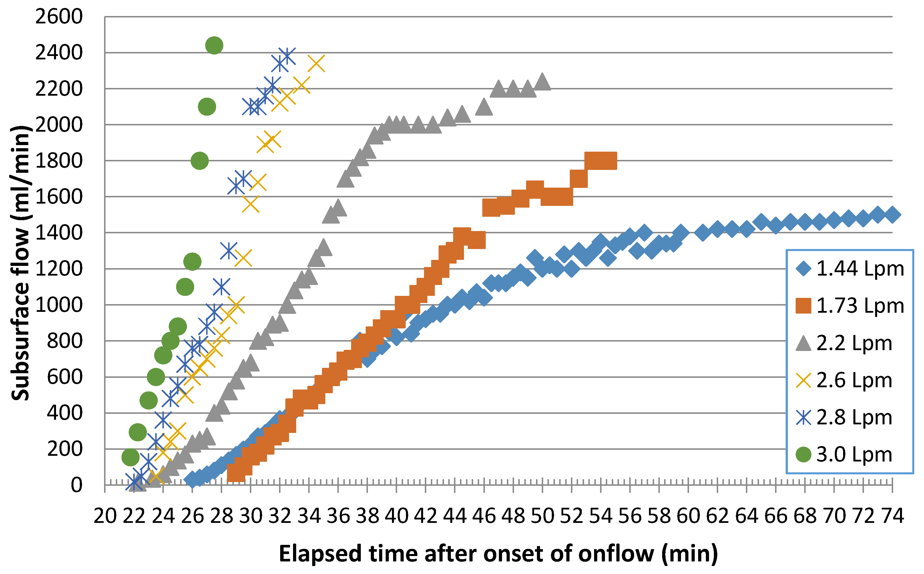
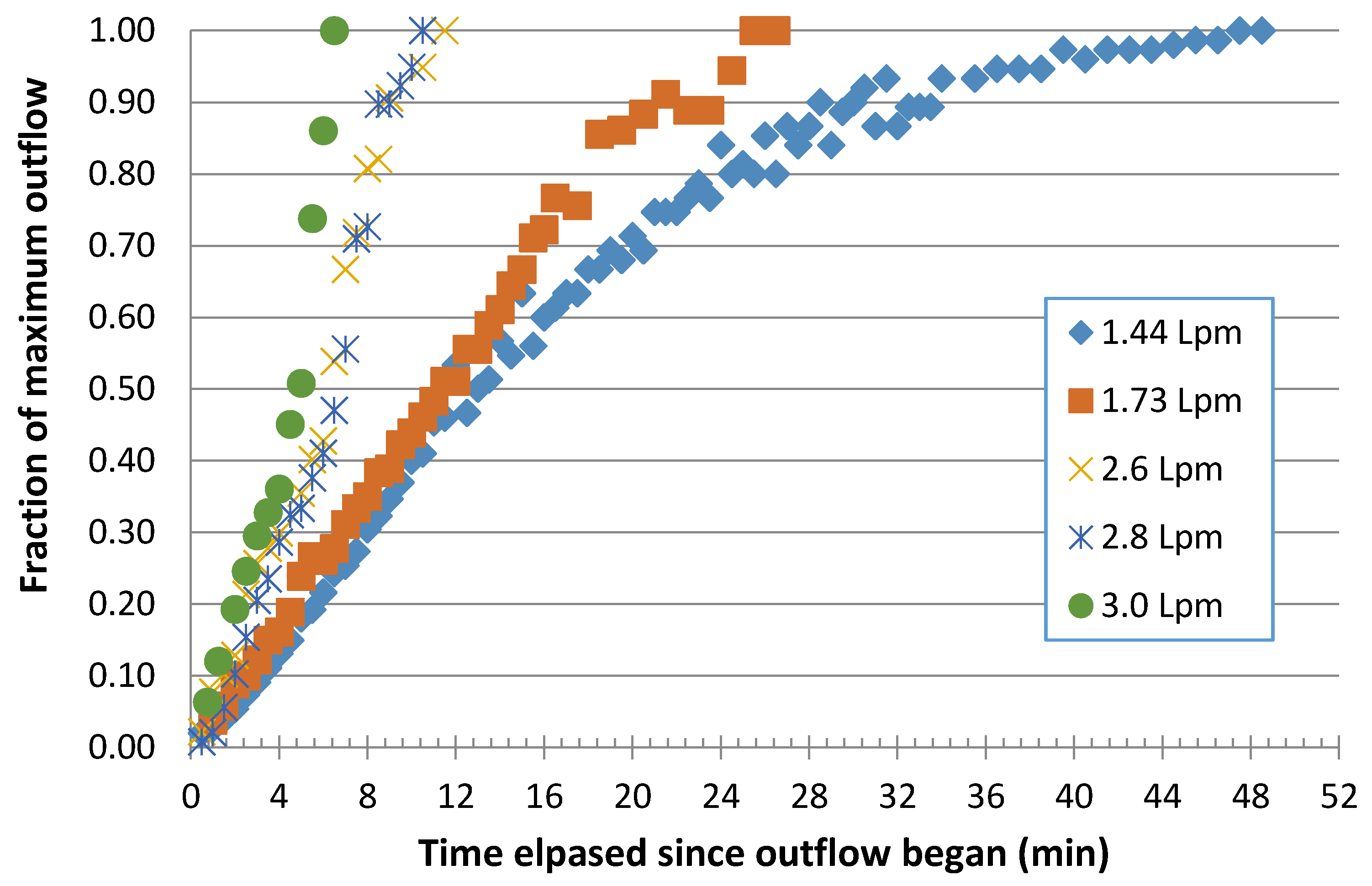
Though three sand depths were used, here we consider the sandbox experiment results from the middle 143 mm depth as those from the other two depths were similar. Figure 6 and Figure 7 illustrate typical subsurface flow data collected from experiments at the 20.6% and 51.8% slopes, respectively, and a variety of flow rates under the ‘natural drainage’ condition of antecedent sand moisture. Figure 6 shows the relative reproducibility of the sandbox wetting experiments at the 2.9 Lpm onflow rate (i.e., tests C, D and E) as well as the effects of much drier antecedent sand moisture conditions that result in a ten minute delay in the subsurface wetting front center of mass reaching the outlet 2 m downslope. This greater time is that required to fill the additional available pore space; a similar delay in time required for outflow to reach the end of the sandbox occurred with the 215 mm deep sand, while less time was required for the shallower 71 mm sand depth. Of course, smaller onflow rates require greater times to appear as subsurface flows downslope as well, and this dependence is also evident in the data for the steeper slope experiments shown in Figure 6. The data of Figure 6 and Figure 7 can be normalized to some degree by considering the time elapsed since outflow began and using the ratio of the observed to the maximum outflow rate as shown for the 51.8% bed slope in Figure 8.
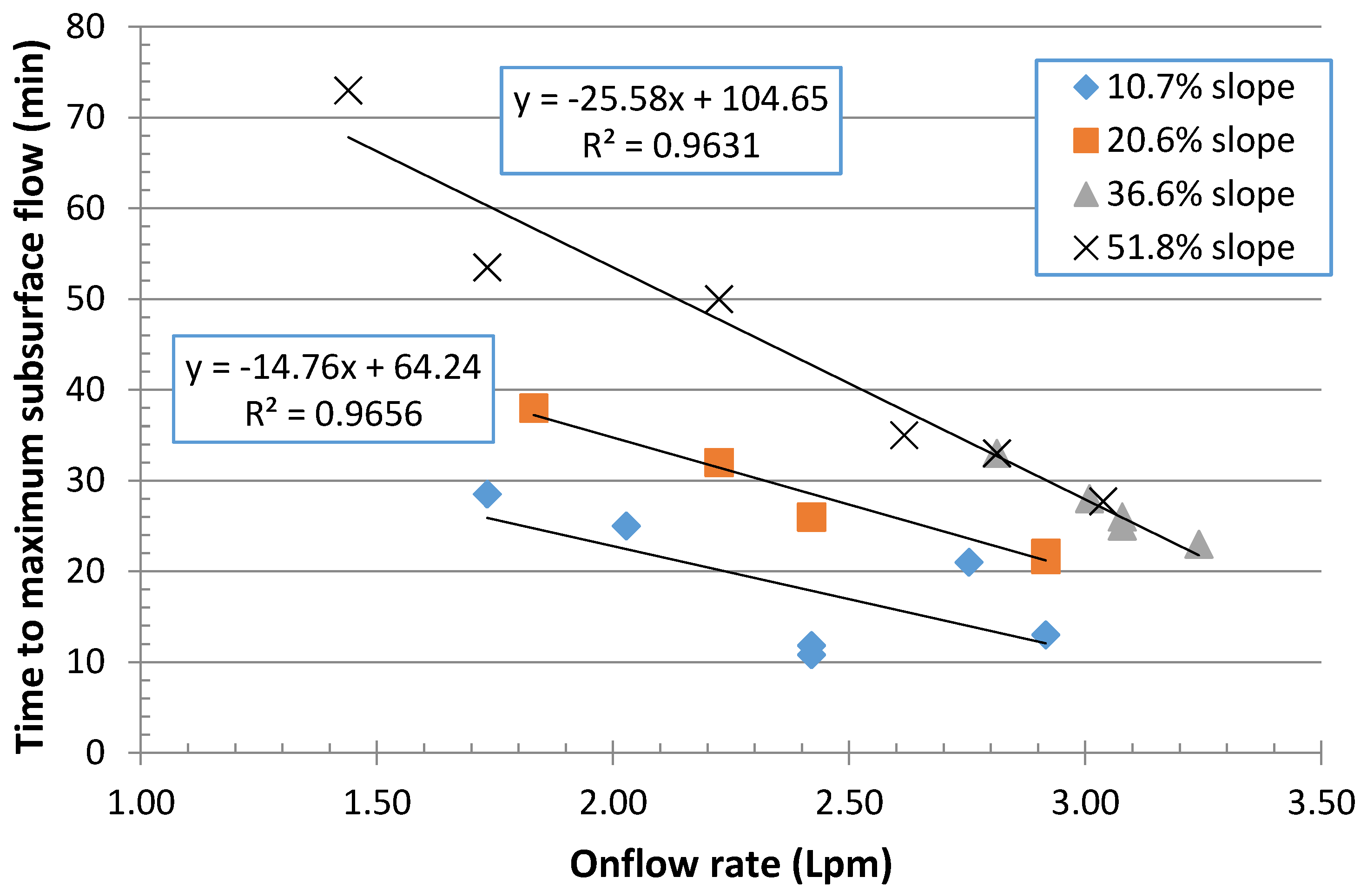
Estimating effective drainable porosities in the field or in hillslope model simulations of course depends on the soil moisture storage achieved in the hillslope, while wetting as well as the drainage rate both function related to the water retention characteristics of the soil. In the sandbox experiments, we found that the degree of wetting was a function of the bedslope (and sand thickness), and this degree of wetted sand could be inferred from the time required to reach maximum subsurface outflows. Figure 9 illustrates the dependence of time to maximum outflow on the onflow rate and bedslope. Although seemingly counter-intuitive that increasingly larger slopes with greater driving gradients should result in shorter times to maximum flows, the progressively greater times required by the steeper slopes for a given onflow rate reflect a greater thickness of effective sand saturation achieved as bed slope increased. At bedslopes greater than 36.6%, this effective thickness of saturated sand appears to be the same as similar drainable volumes from the sandbox for these two depths was obtained.
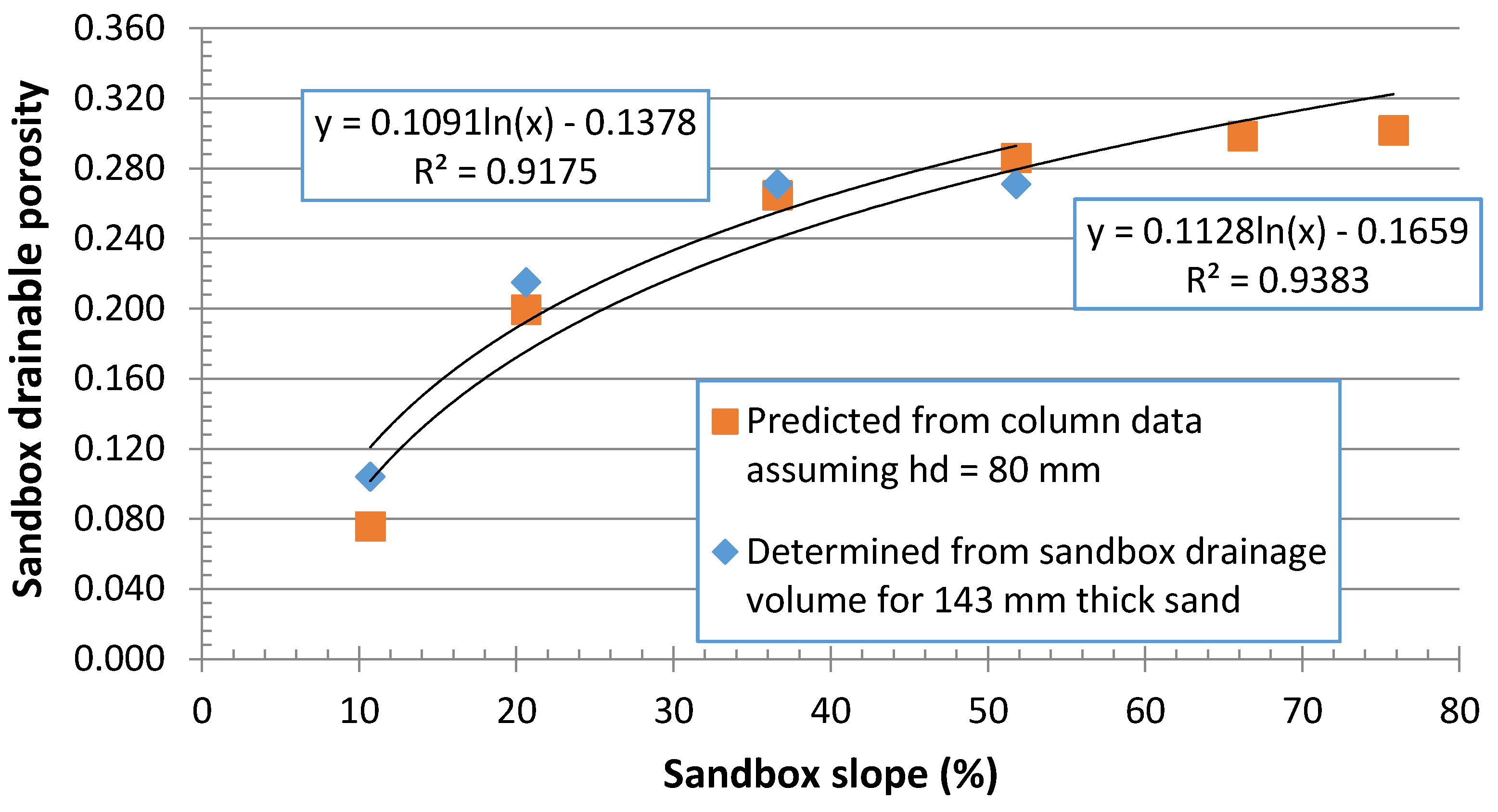
Drainable porosities from the sandbox experiment reflect both the saturation thickness of the sand and its water retention characteristics that both depend on the bedslope of the sandbox. As shown in Figure 9, the increased time to achieve maximum outflow as bedslope increased resulted in greater thicknesses of sand saturation. From Table 2, increased slopes imply effectively ‘taller’ sand columns, resulting in progressively greater capillary pressure heads approaching the top of the sandbox capable of draining ever smaller pore-sizes as bedslope increases. Thus, greater drainable porosities should also occur at progressively steeper slopes with the possibility that the volume available for drainage reaches an upper limit as all the pores accessible to gravitational drainage drain and the thickness of saturated sand remain the same. Using the water retention characteristics of the fine sand summarized in Table 2, as modified using the smaller displacement pressure head (hd = 80 mm), the drainable volume prisms were calculated at the different bedslopes assuming originally saturated sand. These were converted to drainable porosities using the total sand volume and compared with those measured from the ratios of the sandbox total drainage volumes to sand volumes at different slopes as shown in Figure 10. As with the larger hydraulic conductivity associated with the smaller bulk density of the sand within the sandbox experiments as compared to that of the laboratory columns, the simple correction to the smaller displacement pressure head resulted in the predicted and measured drainable being practically equivalent to and having the same trends as the bedslope. Note also that in the sandbox experiments, consistent with the notion of equivalent saturated sand thickness from Figure 8, the drainable porosities of the 36.6% and 51.8% slopes are the same at ~27%, a value quite similar to the maximum predicted possible of ~29%.
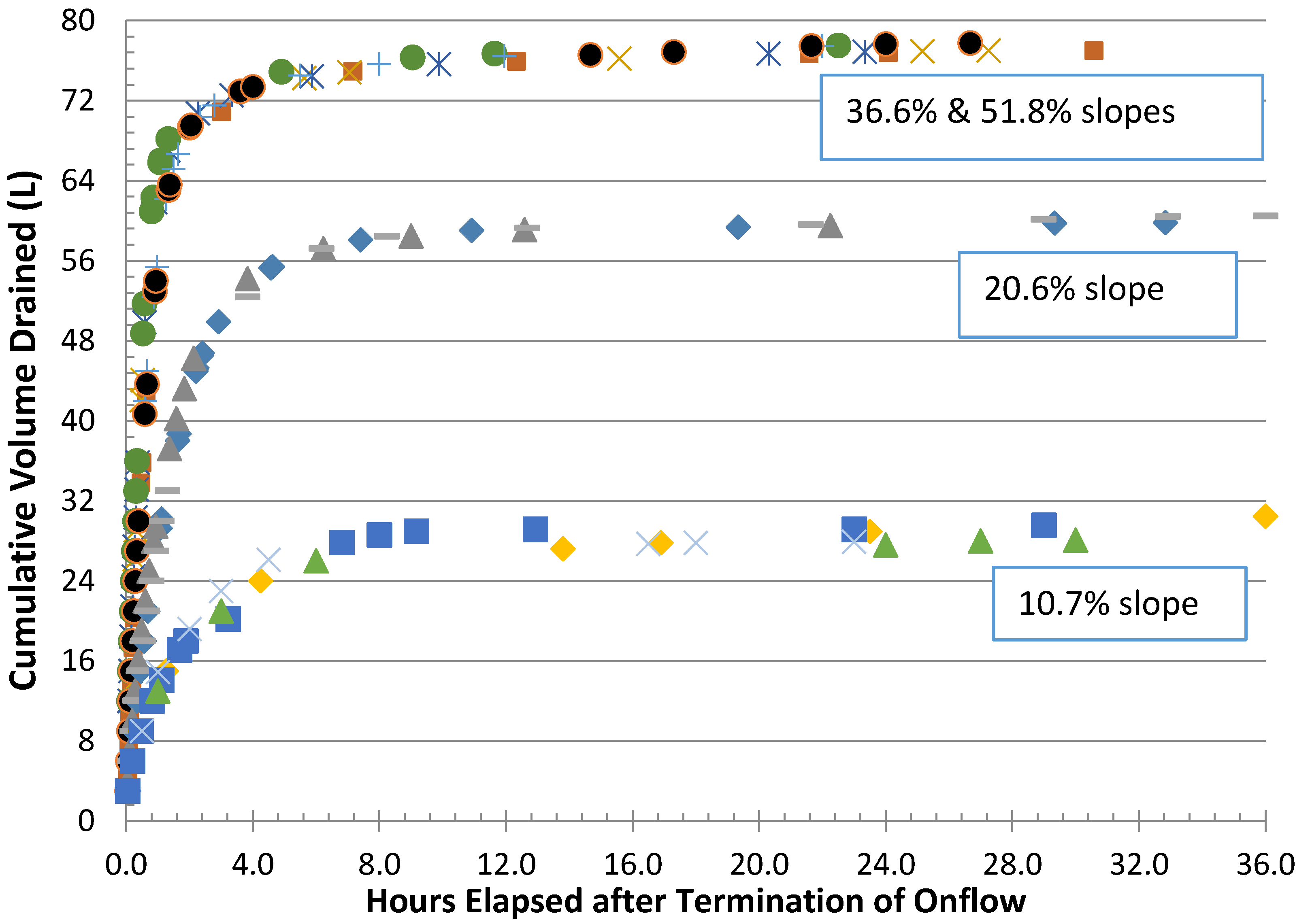
In addition to quantifying drainable porosities and volumes, from a stream recharge perspective, the rates at which soil wet up and drain are equally important to hydrologic connectivity as discussed above. Figure 6 and Figure 7 indicate that in the sandbox experiments, the sand saturated relatively quickly in less than an hour in general for all onflow rates or slopes. Figure 11 illustrates that the drainage rates were not as rapid, requiring approximately 4, 6 and 8 h, respectively, for bedslopes of >36.6%, 20.6% and 10.7% to reach >90% of drainable volume and then upwards to 36 h for complete drainage.
4. Summary and Conclusions—Impacts on Watershed Modeling Efforts
Physical watershed modeling based on continuity and kinematic wave equations for surface and subsurface runoff that include parameterization for the subsurface soil properties, surface topography and roughness and surface-subsurface exchange through a thin surface boundary layer have progressed considerably in the past two decades. The understood goal of such models is to a priori predict surface and subsurface flows to stream channels as a result of rainfall and eventually snow-melt events with minimal pre-calibration. For example, one of the more widely tested, or calibrated physically–based watershed model is the “integrated watershed model”, InHM, proposed by Loague et al. [45]. This model is fundamentally based on the soil properties of the watershed as controlled by an arbitrarily thin surface-subsurface exchange layer. The model incorporates the Manning’s overland flow equation into the diffusive kinematic-wave equation to estimate surface flow depths and velocities. Mirus and others (e.g., [1,2]) provide example ‘maps’ of surface flow depths generated by this model typically in the range of 0.01–1 mm for most of the watershed areas considered. Writing that such shallow flow depths “are of limited relevance in natural systems with the exception of severely disturbed landscapes”, Mirus and Loague [1] borrow the concept of a threshold critical shear stress used in erosion modeling to be used as a measure of when surface flows become relevant. From these calculated flow depths and storm event generated overland flow rates (either infiltration of saturation excess), Mirus and Loague [1] calculate the associated overland flow velocities needed to determine travel times to stream channels as well as critical shear stresses. Nowhere do they note that the flow rates and depths correspond to Reynolds numbers well below the 500 criteria marking the transition between laminar and turbulent flow conditions. Similarly, rainfall and runoff simulation field plot tests in the Lake Tahoe Basin [40] resulted in sheet flow rates in excess of those occurring ‘naturally’ or as would have been modeled as well and these still corresponded to Reynolds numbers at least an order of magnitude less than the 500 assumed to mark the distinction between laminar and turbulent overland flows. Thus, it seems critical to clearly identify that many overland flows, whether modeled or measured in the field, are more properly characterized as laminar rather than turbulent; this critical distinction appears to have several possible effects in modeling efforts. Here, we build on the field observations of overland flow rates and depths in forest and grassland soils, we develop the appropriate laminar flow velocities and celerities and then compare those to measured values using a 1 m wide by 2 m long flume with varying surface roughness conditions and onflow rates. We also then compare flow depths, velocities and celerities associated with assumptions of laminar and turbulent sheet flows showing when they may be similar and underscoring that under field conditions they are not.
For a range of onflow rates (roughly 30–60 mm2/s) and bed slopes (10%–66%) with varying sand roughness depths, we found that all flow depths were predicted by laminar flow equations and that equivalent Manning’s n values were depth dependent and quite small as compared to those used in watershed modeling studies. For example, as indicated in Figure 3 and Figure 4, for a range of large overland flow rates and n = 0.35 typically assumed in the InHM model applications for relatively smooth surface conditions, the laminar flow velocities were 4–5 times greater, while the laminar flow depths were 4–5 times smaller as compared to those estimated from the Manning’s equation. This gross under-estimation of the overland flow velocities of course would result in an over-estimation of travel times for surface flows to reach defined channels and under-estimation of associated shear stresses for estimation of erosion rates using stream power concepts. Without the rainfall and runoff simulation to provide insight into actual flow depths and velocities, this work would not have been possible, which enables determination of the importance of clarifying flow regimes in watershed modeling.
In the sandbox runoff experiments, we were unable to establish overland sheet flow at any onflow rate employed and changed our focus to estimation of the drainability aspects of hillslope as it pertains to watershed connectivity. It appeared in these experiments that infiltration excess runoff can only be generated by a combination of near surface factors that include wettability, surface microtopography and infiltration rates that will require further study using finer-textured soils. With correction of the laboratory measured fine-sand water retention function that involved use of a smaller displacement pressure head, the sandbox drainage characteristics could be predicted including drainage rates and drainable porosities that ranged from about 8%–29% for slopes of 10 to 66%, respectively. It would appear that from a hillslope modeling perspective, it is important to assess the actual displacement pressure head (hydraulic conductivity; see Grismer, [40,44]) of the shallow soils to capture the water retention and drainage characteristics of the hillslope. We found that determination of the displacement pressure head and an assumption of Brooks-Corey pore-size distribution values between 2 and 3 for loamy to sandy soils, respectively, it was possible to adequately capture the water retention and drainable porosity characteristics for modeling purposes.
How should watershed modeling proceed from these observations outlined above? At least perhaps we should note that (a) laminar overland-interflow dominates in less disturbed grassland/forest areas where infiltration rates are high whether or not slopes are steep, and (b) separate overland-interflow zones that are modeled as laminar processes from concentrated flow lines (e.g., determined from GIS based flow paths) modeled as turbulent flows. Further, it is crucial to verify basic field assumptions of processes wherever possible using field measurement techniques such as rainfall and runoff simulation methods.
Conflicts of Interest
The authors declare no conflict of interest.
References
- Mirus, B.B.; Ebel, B.A.; Heppner, C.S.; Loague, K. Assessing the detail needed to capture rainfall-runoff dynamics with physics-based hydrologic-response simulation. Water Resour. Res. 2011, 47, W00H10. [Google Scholar] [CrossRef]
- Mirus, B.B.; Loague, K. How runoff begins (and ends): Characterizing hydrologic response at the catchment scale. Water Resour. Res. 2013, 49, 1–20. [Google Scholar] [CrossRef]
- Jencso, K.G.; McGlynn, B.L. Hierarchical controls on runoff generation: Topographically driven hydrologic connectivity, geology, and vegetation. Water Resour. Res. 2011, 47, W11527. [Google Scholar] [CrossRef]
- Grismer, M.E. Detecting Soil Disturbance/Restoration effects on Stream Sediment Loading in the Tahoe Basin—Modeling Predictions. Hydrol. Proc. 2012, 28, 161–170. [Google Scholar] [CrossRef]
- Grismer, M.E. Erosion Modeling for Land Management in the Tahoe Basin, USA: Scaling from plots to small forest catchments. Hydrol. Sci. J. 2012, 57, 1–20. [Google Scholar] [CrossRef]
- Grismer, M.E.; Shnurrenberger, C.; Arst, R.; Hogan, M.P. Integrated Monitoring and Assessment of Soil Restoration Treatments in the Lake Tahoe Basin. Environ. Monit. Assess. 2009, 150, 365–383. [Google Scholar] [CrossRef] [PubMed]
- Grismer, M.E.; Hogan, M.P. Evaluation of Revegetation/Mulch Erosion Control Using Simulated Rainfall in the Lake Tahoe Basin: 1. Method Assessment. Land Degrad. Dev. 2013, 15, 573–588. [Google Scholar] [CrossRef]
- Grismer, M.E.; Hogan, M.P. Evaluation of Revegetation/Mulch Erosion Control Using Simulated Rainfall in the Lake Tahoe Basin: 2. Bare Soil Assessment. Land Degrad. Dev. 2005, 16, 397–404. [Google Scholar] [CrossRef]
- Grismer, M.E.; Hogan, M.P. Evaluation of Revegetation/Mulch Erosion Control Using Simulated Rainfall in the Lake Tahoe Basin: 3. Treatment Assessment. Land Degrad. Dev. 2005, 16, 489–501. [Google Scholar] [CrossRef]
- Ohara, N.; Kavvas, M.; Easton, D.; Dogrul, E.; Yoon, J.; Chen, Z. Role of snow in runoff processes in a subalpine hillslope: Field study in the Ward Creek Watershed, Lake Tahoe, California, during 2000 and 2001 water years. ASCE J. Hydrol. Eng. 2011, 16, 521–533. [Google Scholar] [CrossRef]
- Ebel, B.A.; Loague, K.; VanderKwaak, J.E.; Dietrich, W.E.; Montgomery, D.R.; Torres, R.; Anderson, S.P. Near-surface hydrologic response for a steep, unchanneled catchment near Coos Bay, Oregon: 2. Physics-based simulations. Am. J. Sci. 2007, 307, 709–748. [Google Scholar] [CrossRef]
- Ebel, B.A.; Loague, K.; Dietrich, W.E.; Montgomery, D.R.; Torres, R.; Anderson, S.P.; Giambelluca, T.W. Near-surface hydrologic response for a steep, unchanneled catchment near Coos Bay, Oregon: 1. Sprinkling experiments. Am. J. Sci. 2007, 307, 678–708. [Google Scholar] [CrossRef]
- Loague, K.; VanderKwaak, J.E. Simulating hydrologic-response for the R-5 catchment: Comparison of two models and the impact of the roads. Hydro. Process. 2002, 16, 1015–1032. [Google Scholar] [CrossRef]
- Loague, K.; Heppner, C.S.; Ebel, B.A.; VanderKwaak, J.E. The quixotic search for a comprehensive understanding of hydrologic response at the surface: Horton, Dunne, Dunton, and the role of concept development simulations. Hydrol. Proc. 2010, 24, 2499–2505. [Google Scholar] [CrossRef]
- Berger, C.; Schulze, M.; Rieke-Zapp, D.; Schlunegger, F. Rill development and soil erosion: A laboratory study of slope and rainfall intensity. Earth Surf. Proc. Land. 2010, 35, 1456–1467. [Google Scholar] [CrossRef]
- Tauro, F.; Grimaldi, S.; Petroselli, A.; Rulli, M.C.; Porfiri, M. Fluorescent particle tracers in surface hydrology: A proof of concept in a semi-natural hillslope. Hydrol. Earth Syst. Sci. 2012, 16, 2973–2983. [Google Scholar] [CrossRef]
- Ticehurst, J.L.; Cresswell, H.P.; McKenzie, N.J.; Glover, M.R. Interpreting soil and topographic properties to conceptualise hillslope hydrology. Geoderma 2007, 137, 279–292. [Google Scholar] [CrossRef]
- Carr, A.; Loague, K.; VanderKwaak, J.E. Hydrologic-response simulations for the North Fork of Caspar Creek: Second growth, clearcut, new growth, and CWE scenarios. Hydrol. Proc. 2014, 28, 1476–1494. [Google Scholar] [CrossRef]
- Lee, J.; Feng, X.; Faiia, A.; Posmentier, E.; Osterhuber, R.; Kirchner, J. Isotopic evolution of snowmelt: A new model incorporating mobile and immobile water. Water Resour. Res. 2010, 46, W11512. [Google Scholar] [CrossRef]
- VanderKwaak, J.E.; Loague, K. Hydrologic-response simulations for the R-5 catchment with a comprehensive physics-based model. Water Resour. Res. 2001, 37, 999–1013. [Google Scholar] [CrossRef]
- Jencso, K.G.; McGlynn, B.L.; Gooseff, M.N.; Wondzell, S.M.; Bencala, K.E.; Marshall, L.A. Hydrologic connectivity between landscapes and streams: Transferring reach-and plot-scale understanding to the catchment scale. Water Resour. Res. 2009, 45, W04428. [Google Scholar] [CrossRef]
- Vidon, P.G.F.; Hill, A.R. Landscape controls on nitrate removal in stream riparian zones. Water Resour. Res. 2004, 40, W03201. [Google Scholar] [CrossRef]
- Ocampo, C.J.; Sivapalan, M.; Oldham, C. Hydrological connectivity of upland-riparian zones in agricultural catchments: Implications for runoff generation and nitrate transport. J. Hydrol. 2006, 331, 643–658. [Google Scholar] [CrossRef]
- McGlynn, B.L.; McDonnell, J.J. Quantifying the relative contributions of riparian and hillslope zones to catchment runoff. Water Resour. Res. 2003, 39, 1310. [Google Scholar] [CrossRef]
- McGlynn, B.L.; McDonnell, J.J. Role of discrete landscape units in controlling catchment dissolved organic carbon dynamics. Water Resour. Res. 2003, 39, 1090. [Google Scholar] [CrossRef]
- Carlyle, G.C.; Hill, A.R. Groundwater phosphate dynamics in a river riparian zone: Effects of hydrologic flowpaths, lithology, and redox chemistry. J. Hydrol. 2001, 247, 151–168. [Google Scholar] [CrossRef]
- Jencso, K.G.; McGlynn, B.L.; Gooseff, M.N.; Bencala, K.E.; Wondzell, S.M. Hillslope hydrologic connectivity controls riparian groundwater turnover: Implications of catchment structure for riparian buffering and stream water sources. Water Resour. Res. 2010, 46, W10524. [Google Scholar] [CrossRef]
- Dunne, T.; Black, R.D. Partial area contributions to storm runoff in a small New England watershed. Water Resour. Res. 1970, 6, 1296–1311. [Google Scholar] [CrossRef]
- Anderson, M.G.; Burt, T.P. The role of topography in controlling throughflow generation. Earth Surf. Process. Landf. 1978, 3, 331–334. [Google Scholar] [CrossRef]
- Beven, K.J. The hydrological response of headwater and sideslope areas. Hydrol. Sci. Bull. 1978, 23, 419–437. [Google Scholar] [CrossRef]
- Burt, T.P.; Butcher, D.P. Topographic controls of soil moisture distributions. J. Soil Sci. 1985, 36, 469–486. [Google Scholar] [CrossRef]
- Savenije, H.H.G. Topography driven conceptual modeling, FLEX-Topo. Hydrol. Earth Syst. Sci. 2010, 14, 2681–2692. [Google Scholar] [CrossRef]
- Sidle, R.C.; Tsuboyama, Y.; Noguchi, S.; Hosoda, I.; Fujieda, M.; Shimizu, T. Stormflow generation in steep forested headwaters: A linked hydrogeomorphic paradigm. Hydrol. Proc. 2000, 14, 369–385. [Google Scholar] [CrossRef]
- McGlynn, B.L.; McDonnell, J.J.; Seibert, J.; Kendall, C. Scale effects on headwater catchment runoff timing, flow sources, and groundwater-streamflow relations. Water Resour. Res. 2004, 40, W07504. [Google Scholar] [CrossRef]
- McGuire, K.J.; McDonnell, J.J.; Weiler, M.; Kendall, C.; McGlynn, B.L.; Welker, J.M.; Seibert, J. The role of topography on catchment-scale water residence time. Water Resour. Res. 2005, 41, W05002. [Google Scholar] [CrossRef]
- Tetzlaff, D.; Seibert, J.; McGuire, K.J.; Laudon, H.; Burns, D.A.; Dunn, S.M.; Soulsby, C. How does landscape structure influence catchment transit times across different geomorphic provinces? Hydrol. Proc. 2009, 23, 945–953. [Google Scholar] [CrossRef]
- Hewlett, J.D.; Hibbert, A.R. Factors affecting the response of small watersheds to precipitation in humid areas. In Forest Hydrology; Sopper, W.E., Lull, H.W., Eds.; Pergamon: New York, NY, USA, 1967; pp. 275–291. [Google Scholar]
- Harr, R.D. Water flux in soil and subsoil on a steep forested slope. J. Hydrol. 1977, 33, 37–58. [Google Scholar] [CrossRef]
- Hopp, L.; McDonnell, J.J. Connectivity at the hillslope scale: Identifying interactions between storm size, bedrock permeability, slope angle and soil depth. J. Hydrol. 2009, 376, 378–391. [Google Scholar] [CrossRef]
- Grismer, M.E. Determination of watershed infiltration and erosion parameters from field Rainfall Simulation analyses. Hydrology 2016. submitted. [Google Scholar]
- Benjamin, T.B. Wave formation in laminar flow down an inclined plane. J. Fluid Mech. 1957, 2, 554–574. [Google Scholar] [CrossRef]
- Singh, V.P. Is hydrology kinematic? Hydrol. Proc. 2002, 16, 667–716. [Google Scholar] [CrossRef]
- Loague, K. Rainfall-Runoff Modeling, in IAHS Benchmark Papers in Hydrology; McDonnell, J.J., Ed.; IAHS Press: Wallingford, UK, 2010; Volume 4, p. 506. [Google Scholar]
- Grismer, M.E. Pore-size distribution and infiltration. Soil Sci. 1986, 141, 249–260. [Google Scholar] [CrossRef]
- Loague, K.; Heppner, C.S.; Mirus, B.B.; Ebel, B.A.; Ran, Q.; Carr, A.E.; BeVille, S.H.; VanderKwaak, J.E. Physics-based hydrologic response simulation: Foundation for hydroecology and hydrogeomorphology. Hydrol. Proc. 2006, 20, 1231–1237. [Google Scholar] [CrossRef]
Figure 1.
Diagram of undisturbed steady laminar flow down an inclined plane with parameter definitions.
Figure 1.
Diagram of undisturbed steady laminar flow down an inclined plane with parameter definitions.

Figure 2.
Photo of runoff simulator with 143 mm fine sand depth.

Figure 3.
Dependence of the wave celerity on laminar or turbulent flow assumptions for 0.2 mm (a) and 0.5 mm (b) flow depth and Manning’s n = 0.30.
Figure 3.
Dependence of the wave celerity on laminar or turbulent flow assumptions for 0.2 mm (a) and 0.5 mm (b) flow depth and Manning’s n = 0.30.

Figure 4.
Dependence of overland flow mean velocities (Q = 20 mm2/s) on slope for laminar and turbulent (Manning’s equation) flow and different roughness values.
Figure 4.
Dependence of overland flow mean velocities (Q = 20 mm2/s) on slope for laminar and turbulent (Manning’s equation) flow and different roughness values.

Figure 5.
Dependence of the ratio of Manning’s number to laminar predicted flow depths (or velocities) on overland flow rate for a 20% slope and different roughness values.
Figure 5.
Dependence of the ratio of Manning’s number to laminar predicted flow depths (or velocities) on overland flow rate for a 20% slope and different roughness values.

Figure 6.
Sandbox subsurface outflow rate at 2 m downslope as it depends on elapsed time after onset of onflow at rates listed for 20.6% bed slope and 143 mm depth sand. All tests under conditions of previous ‘natural drainage’ except as indicated for the ‘dry’ sand case at 2.9 Lpm.
Figure 6.
Sandbox subsurface outflow rate at 2 m downslope as it depends on elapsed time after onset of onflow at rates listed for 20.6% bed slope and 143 mm depth sand. All tests under conditions of previous ‘natural drainage’ except as indicated for the ‘dry’ sand case at 2.9 Lpm.

Figure 7.
Sandbox subsurface outflow rate at 2 m downslope as it depends on elapsed time after onset of onflow at rates listed for 51.8% bed slope and 143 mm depth sand. All tests under conditions of previous ‘natural drainage’.
Figure 7.
Sandbox subsurface outflow rate at 2 m downslope as it depends on elapsed time after onset of onflow at rates listed for 51.8% bed slope and 143 mm depth sand. All tests under conditions of previous ‘natural drainage’.

Figure 8.
Sandbox subsurface outflow rate as it depends on elapsed time after beginning at 2 m downslope for bed slope of 51.8% and 143 mm depth sand.
Figure 8.
Sandbox subsurface outflow rate as it depends on elapsed time after beginning at 2 m downslope for bed slope of 51.8% and 143 mm depth sand.

Figure 9.
Time to maximum subsurface outflow rate as it depends on onflow rate for 143 mm depth sand at four different slopes.
Figure 9.
Time to maximum subsurface outflow rate as it depends on onflow rate for 143 mm depth sand at four different slopes.

Figure 10.
Predicted and measured drainable porosities as they depend on bedslope for 143 mm sand depth.
Figure 10.
Predicted and measured drainable porosities as they depend on bedslope for 143 mm sand depth.

Figure 11.
Measured rates of drainage as they depend on bedslope for 143 mm sand depth.


| Slope (%) | Q (mm2/s) | Re | Predicted hlaminar (mm) | Bare Aluminum hmeas (mm) | #60 1 sandpaper hmeas (mm) | Apparent n |
|---|---|---|---|---|---|---|
| 10.7 | 26.7 | 24 | 0.44 | 0.43–0.45 | 0.41–0.44 | 0.024 |
| 37.5 | 34 | 0.49 | 0.48–0.50 | 0.46–0.49 | 0.024 | |
| 46.7 | 42 | 0.53 | 0.52–0.54 | 0.50–0.53 | 0.024 | |
| 57.2 | 51 | 0.57 | 0.56–0.58 | 0.54–0.57 | 0.023 | |
| 20.6 | 26.7 | 24 | 0.36 | 0.35–0.37 | 0.33–0.36 | 0.029 |
| 37.5 | 34 | 0.40 | 0.39–0.41 | 0.37–0.39 | 0.026 | |
| 46.7 | 42 | 0.43 | 0.42–0.44 | 0.4–0.43 | 0.024 | |
| 57.2 | 51 | 0.46 | 0.45–0.47 | 0.44–0.47 | 0.022 | |
| 36.6 | 26.7 | 24 | 0.30 | 0.29–0.31 | 0.27–0.30 | 0.033 |
| 37.5 | 34 | 0.33 | 0.32–0.34 | 0.30–0.33 | 0.029 | |
| 46.7 | 42 | 0.36 | 0.35–0.37 | 0.33–0.36 | 0.026 | |
| 57.2 | 51 | 0.38 | 0.34–0.39 | 0.35–0.38 | 0.023 | |
| 51.8 | 26.7 | 24 | 0.27 | 0.26–0.28 | NA 2 | 0.028 |
| 37.5 | 34 | 0.30 | 0.29–0.30 | NA | 0.027 | |
| 46.7 | 42 | 0.32 | 0.31–0.33 | NA | 0.025 | |
| 57.2 | 51 | 0.35 | 0.34–0.36 | NA | 0.023 | |
| 66.2 | 26.7 | 24 | 0.25 | 0.22–0.26 | NA | 0.031 |
| 37.5 | 34 | 0.28 | 0.27–0.30 | NA | 0.029 | |
| 46.7 | 42 | 0.31 | 0.30–0.32 | NA | 0.028 | |
| 57.2 | 51 | 0.33 | 0.32–0.35 | NA | 0.025 |
1 Results for finer 100 and 150 grit sandpaper were the same as those for bare aluminum; 2 Uniform width flow could not be established for the steep slopes on the sandpaper (i.e., fingered flow).
| Capillary Pressure Head (mm) | Volumetric Water Content 1 (m3/m3) | Apparent Specific Yield (%) |
|---|---|---|
| 10–50 | 0.40 2 | 0 |
| 60–80 | 0.36 | 0 |
| 100 | 0.36 | 0 |
| 120 | 0.36 | 0 |
| 140 | 0.34 | 0.02 |
| 160 | 0.33 | 0.42 |
| 180 | 0.33 | 0.74 |
| 200 | 0.29 | 1.3 |
| 220 | 0.22 | 2.5 |
| 240 | 0.18 | 3.8 |
| 260 | 0.15 | 5.1 |
| 280 | 0.13 | 6.4 |
| 300 | 0.10 | 7.7 |
| 320 | 0.09 | 8.9 |
| 340 | 0.07 | 10.1 |
| 360 | 0.06 | 11.2 |
| 380 | 0.05 | 12.2 |
| 400 | 0.04 | 13.2 |
1 Five column average values at average bulk density of 1700 kg/m3; 2 Exceeds average porosity and value reflects “free-water” in column ring.
© 2016 by the author; licensee MDPI, Basel, Switzerland. This article is an open access article distributed under the terms and conditions of the Creative Commons Attribution (CC-BY) license (http://creativecommons.org/licenses/by/4.0/).
Share and Cite
MDPI and ACS Style
Grismer, M.E. Surface Runoff in Watershed Modeling—Turbulent or Laminar Flows? Hydrology 2016, 3, 18. https://doi.org/10.3390/hydrology3020018
AMA Style
Grismer ME. Surface Runoff in Watershed Modeling—Turbulent or Laminar Flows? Hydrology. 2016; 3(2):18. https://doi.org/10.3390/hydrology3020018
Chicago/Turabian StyleGrismer, Mark E. 2016. "Surface Runoff in Watershed Modeling—Turbulent or Laminar Flows?" Hydrology 3, no. 2: 18. https://doi.org/10.3390/hydrology3020018
Note that from the first issue of 2016, this journal uses article numbers instead of page numbers. See further details here.