A Multi-Faceted Debris-Flood Hazard Assessment for Cougar Creek, Alberta, Canada

Abstract

A destructive debris flood occurred between 19 and 21 June 2013 on Cougar Creek, located in Canmore, Alberta. Cougar Creek fan is likely the most densely developed alluvial fan in Canada. While no lives were lost, the event resulted in approximately $40 M of damage and closed both the Trans-Canada Highway (Highway 1) and the Canadian Pacific Railway line for a period of several days. The debris flood triggered a comprehensive hazard assessment which is the focus of this paper. Debris-flood frequencies and magnitudes are determined by combining several quantitative methods including photogrammetry, dendrochronology, radiometric dating, test pit logging, empirical relationships between rainfall volumes and sediment volumes, and landslide dam outburst flood modeling. The data analysis suggests that three distinct process types act in the watershed. The most frequent process is normal or “clearwater” floods. Less frequent but more damaging are debris floods during which excessive amounts of bedload are transported on the fan, typically associated with rapid and extensive bank erosion and channel infilling and widening. The third and most destructive process is interpreted to be landslide dam outbreak floods. This event type is estimated to occur at return periods exceeding 300 years. Using a cumulative magnitude frequency technique, the data for conventional debris floods were plotted up to the 100–300s year return period. A peak-over-threshold approach was used for landslide dam outbreak floods occurring at return periods exceeding 300 years, as not all such events were identified during test trenching. Hydrographs for 6 return period classes were approximated by using the estimated peak discharges and fitting the hydrograph shape to integrate to the debris flood volumes as determined from the frequency-magnitude relationship. The fan volume was calculated and compared with the integrated frequency-magnitude curve to check of the validity of the latter. A reasonable match was accomplished, verifying the overall relationship. The findings from this work were later used as input to a risk assessment seeking to quantify risk to loss of life and economic losses. The risk assessment then formed the basis for design of debris-flood mitigation structures.

1. Introduction

The southwestern Alberta mountain front was affected by a high intensity/duration rainstorm between 19 and 21 June 2013. Direct runoff, coupled with meltwater released from rain on a shallow snowpack, caused sudden and prolonged high flows in the Bow, High, and Ghost Rivers and their tributaries originating in the Rocky Mountains. These flows resulted in high rates and volumes of sediment transport, bank erosion and avulsions on alluvial fans.

Almost all of the steep gradient tributaries to Bow River within the municipal boundary of the Town of Canmore (Town) were affected by the combined storm and snowmelt runoff, including Cougar Creek (Figure 1). Major damage was sustained on Cougar Creek fan due to sediment deposition and bank erosion along the principal channel which is flanked by dense development. Economic damages were in excess of CDN $40 million for emergency assessments and reconstruction costs alone (Alberta Transportation [1], ISL Engineering [2]). This cost estimate does not include additional costs such as services provided by the fire department (e.g., time, food, or equipment), town staff (e.g., overtime, benefits, food, clothes, and equipment), or any costs associated with flood relief accommodations.

Some 9 million m³ of rain (220 mm) fell on the 43 km² watershed of Cougar Creek over the course of the 3-day storm, a total that was augmented by snowmelt. This storm event led to high peak flows and extensive sediment aggradation along Cougar Creek both upstream of the fan apex and on the fan reaches, which was accompanied by lateral instability on the fan as the channel lost confinement and eroded prior bank protection measures. The peak flow of the debris flood appeared to have exceeded at least five times the estimated 100-year return period flood of 16 m³/s (AMEC [3]).

The channel aggradation allowed the streamflow to overtop the confines of the previously confined channel which led to flood waters eroding banks past property lines, undermining buildings foundations and destroying the support of decks and supported balconies. No buildings on Cougar Creek fan were completely destroyed by the event, but a number of them suffered major damage. The 9.5 m wide, elliptical culvert under Elk Run Boulevard on the upper fan sustained damage, but survived thanks to continuous excavation of debris by the Town of Canmore and its emergency contractors during the event which threatened to block the culvert. No creek avulsion occurred until the creek reached Highway 1 on the lower third of the fan, where the existing box culverts were blocked by sediment and woody debris. Such an avulsion further upstream would have led to significantly more damage to buildings and infrastructure than was observed. The blocked culverts at Highway 1 resulted in flows avulsing over the highway and down the median to the east (Figure 2). These overflows resulted in portions of the highway being undermined and collapsing. The box culverts at Highway 1A and CP Rail further downstream were also blocked by sediment and debris, the latter of which was out of commission for approximately three days until it was repaired.

Alluvial fan hazard assessments have a rich history worldwide and in Canada (Jakob and Hungr [4]). Risk assessments, in contrast, are much rarer with only a handful of such studies published in the global literature (Dai et al. [5]). In terms of the management response to a known alluvial hazard, two approaches are typical: a fixed return period is chosen as the design event or a quantitative risk assessment (QRA) is conducted. The former is the most common approach adopted by decision-makers, in part because it is a concept that is easily understood by both the public and policy makers. Once the design event is quantified, the size and scale of the mitigation measures is then selected to protect against the specified design event. A drawback of this approach is that the consequences of the hazard are not systematically quantified across a range of return periods. The other approach is risk-based: a wide spectrum of hazard scenarios and return periods is considered, and risk to loss of life or economic risk is then estimated and compared against risk tolerance thresholds. Risk is subsequently reduced through landuse decisions or engineered structures to tolerable or acceptable risk levels. Hybrid methods exist. A comprehensive summary of various approaches in Europe is presented by Rudolf-Miklau et al. [6]. At this time, QRAs are still the exception in Canada but are gaining popularity amongst practitioners and regulators alike (Porter et al. [7]). The present study was designed as input to a QRA, on which, ultimately, risk reduction measure decisions are based.

Hazard assessments of debris floods are notoriously challenging as a several variables have to be deciphered that are not readily available through gauged or other regular documentation. Despite these challenges, debris-flood hazard assessments need to be factually correct and be reproducible (i.e., Kienholz [8], PLANAT [9], Rickenmann [10]). To estimate debris-flood magnitudes, the amount of sediment transported and the peak discharge needs to be determined. The former is difficult as hydrologic and hydraulic processes are subject to extreme spatial and temporal variability that are due to sediment availability and co-event input, grain-size distribution, channel geometry and flow depth, and transitions between subcritical and supercritical flow (Hassan et al. [11], Comiti and Moa [12], Church [13]).

As Rickenmann [10] points out, a notable difference exists between what is referred to as mountain “torrents” (<25 km² in size) and mountain rivers (>25 km² in size). The former being often limited in terms of available sediment, while the latter is typically not (Montgomery and Buffington [14], Bovis and Jakob [15]). Cougar Creek has a watershed area of 43.5 km² and is sediment supply unlimited as discussed in Section 2. Exceedance of a critical specific shear stress threshold determines the onset of sediment mobilization in such a steep mountain river. This threshold is a function of channel slope, grain size distribution, and grain shape (i.e., Lamb et al. [16], Recking [17], Rosport [18], Bathurst [19]). Discharge is a function of the hyetograph of the debris-flood triggering storm and numerous exceedances are conceivable during a single storm, depending on the evolution and complexity of the debris-flood triggering hydroclimatic event. The above variables vary in space and time. Compounding this complexity, is that the definition of a representative grain size distribution for the entire stream is often unachievable, as grain size is highly dependent on the origin of sediment. In the case of Cougar Creek, sediment derives from undercutting of adjacent talus slopes, debris flows from steep tributaries, rock slides and erosion of late Pleistocene glacial deposits. Each sediment source displays different properties in terms of its shape and diameter which is either used to determine flow resistance, the start of grain mobilization or transport efficiency. Moreover, during a long-lasting flood with variable hydrograph peaks, the grain size distribution is altered through lateral sediment input and the formation and destruction of surface armor layers. Consequently, and as noted by Rickenmann [10], bedload transport initiation and transport, flow resistance (through grain size variation and woody debris), formation and destruction of armour layers and sediment availability needs to be understood and considered in the quantification of bedload transport. Such methods are summarized concisely by Rickenmann [10], who also provides a summary of one-dimensional and two-dimensional numerical simulation methods.

The above demonstrates that the quantification of bedload transport volumes requires an in-depth understanding of a plethora of variables and their flux in space and time. From a practitioner’s point of view, a balance needs to be struck between the available funds to execute the project and to ascertain reproducibility, quantification of uncertainties and regulatory requirements. Application of sediment transport formulae is possible, albeit difficult in light of the unknown storm hyetographs and the resulting hydrographs as well as channel bed evolution. Moreover, this method will not be applicable to the expected landslide dam outbreak floods originating in the Cougar Creek watershed.

In this paper, we attempt a different approach and combine different methods gleaned from paleoflood hydrology, geomorphology and develop or evolve and apply existing empirical functions to arrive at reasonable estimates of frequency-magnitude relationships of debris floods on Cougar Creek.

2. Study Area

The study area is located on a tributary of Bow River in the southeastern Canadian Rockies approximately 100 km west of Calgary, Alberta. Cougar Creek drains into Bow River at an elevation of about 1400 masl (metres above sea level) and has its highest peak (Mount Townsend) at 2820 masl. The average channel gradient of the mainstem channel is 5.5% for 3 km upstream of the fan apex. This low gradient indicates that Cougar Creek is not susceptible to debris flows along its main channel. However, all tributaries of Cougar Creek are capable of producing debris flows that feed sediment into the Cougar Creek mainstem channel. The watershed is covered by Engelmann spruce and Douglas firs as well as birches and various shrubs up to an elevation of a maximum of 2400 m. Above that elevation, the alpine region is characterized by krummholz and low shrubs. There are no glaciers in the Cougar Creek watershed.

2.1. Bedrock Geology

The Canadian Rocky Mountains (CRM) are a fold and thrust belt, where thick units of more erosion resistant Paleozoic carbonates were folded and thrust progressively in a north-westerly direction over more friable Mesozoic sandstones and shales. Four main sequences of rocks can be characterized in the Canmore region. The oldest unit at the base is referred to as the basement rocks of the North American cratonic plate, which bears no relevance to this present study. The next unit is the Pre-Cambrian to Lower-Cambrian clastic and minor carbonate rock unit composed of weathered rock from the Canadian Shield (further east). The middle carbonate unit (Middle-Cambrian to Upper Jurassic, 540–155 Ma) consists of marine carbonates (limestone and dolostone) and shale. The upper unit is composed of a young Jurassic to Tertiary (155–1.9 Ma) unit of sandstone, shale, conglomerate and coal. This final unit consists of eroded sediments from an uplifting landscape into a foreland basin to the east (Gadd [20] and Henderson et al. [21]).

The geologic exposures within the Cougar Creek drainage are primarily composed of thick Carboniferous and Devonian successions. Most of the rock units are of Lower Carboniferous (Mississippian) origin with some representation of Upper Carboniferous (Pennsylvanian) and Devonian units. Most of the rock formations are sedimentary (carbonates and siliciclastics) with minor metamorphic components (i.e., calcite). Geologic formations that are more resistant to erosion are more conducive to the formation of cliffs, while more recessive units tend form sloping ledges.

2.2. Quaternary Geology

The Cougar Creek watershed is located in a region that was affected by phases of glaciation and de-glaciation during the Holocene period. During this period, the final stages of major glacial erosion and deposition occurred and the present day Quaternary sedimentation in the Bow Valley was established.

Late Pleistocene glaciers reached their maximum extent in the Canadian Rockies around 16,500 years BP after which significant climatic warming led to the decay of the extensive mountain ice sheets (Menounos et al. [22]). Several studies have been conducted on the Pleistocene and Holocene glaciation of the Canadian Rockies. The first series of detailed studies of the region were completed by Rutter in the 1960s and 1970s who originally described four glacial events (Rutter [23,24,25,26]). The events are the Pre-Bow Valley Advance, Bow Valley Advance, Canmore Advance and Eisenhower Junction Advance. Bobrowski and Rutter [27] later discarded the notion of the Pre-Bow Valley Advance.

During the Holocene minor periods of glacial advance and retreat alternated by were restricted to the high elevation icefields and cirques (Reasoner et al. [28]). Such advances provided sediments from eroding moraines to the channel system and locally oversteepened slopes. The lack of morainal deposits in the Cougar Creek watershed can be explained by the high rates of geomorphic activity that eroded most evidence of Holocene glacial advances.

The tributary valleys were likely ice-free when there was still a trunk glacier occupying Bow Valley. This glacier would have created a dam against which ponding would have occurred in the principal tributary valleys. Particularly in low gradient valleys such as Cougar Creek, glaciolacustrine sediments indicate the development of glacially dammed lakes that may have persisted for many years or even centuries. Eventual drainage of these lakes and subsequent erosion has exposed thinly bedded lacustrine sediments in soil outcrops, including along the mainstem channel of Cougar Creek. At times, such lakes would have overtopped the main trunk glacier in the Bow Valley or drained through subglacial conduits, the frequency of which is unknown.

Sediment terraces flank the main valleys of the Canmore area and were interpreted as kame terraces by Rutter [26]. They are composed primarily of fluvial sands and gravels with some lacustrine sediment resulting from glacial meltwater ponding. Since the retreat of the glaciers, the kame terraces, that likely blocked the Cougar Creek drainage, have been eroding and reworked by periodic stream flow and flooding events. As such they provide a contemporary sediment source for Cougar Creek debris floods.

The early Holocene experienced a period of drought called the Hypsithermal that caused the lowering of lake levels, higher treelines and almost complete ablation of glaciers between 10,000 years BP and 9400 years BP. According to studies in lake sediment cores, the glaciers did not re-establish until 6800 years BP (Beierle and Smith [29], Beierle [30]).

The Little Ice Age began around the 1200s and terminated in the mid-1800s. Summit Icefields, valley glaciers and cirques reached their Holocene maximum extent during this period of time (Luckman [31]). Within the Cougar Creek watershed, little evidence of Little Ice Age moraines is observed which is attributed again to the high rates of landslides and erosion that would have removed such evidence over the past century and a half.

3. Fan Development

The alluvial fan of Cougar Creek has an area of 3.1 km² (Figure 1). Almost the entire fan is developed including approximately 1400 residential homes, a light industrial area, an elementary school, a heliport, Highway 1 and 1A, and the Canadian Pacific Railway (CPR) line. Average channel gradients on the fan range between 3% and 5%. Cougar Creek was initially channelized through excavation in the 1950s and 1960s, allowing for the present day dense development. Prior to this period, most of the development was restricted to transportation corridors. Cougar Creek is currently restricted to a narrow corridor that is approximately 100 to 120 m wide, about one-third of which is occupied by the channel.

Most of the colluvial and alluvial fan development occurred in the lower Bow Valley between the retreat of trunk valley ice (~12,000 years BP) and the Hypsithermal (~6000 years BP), as determined by the stratigraphic location of Mazama tephra in the upper sediments of a number of fans (Roed and Wasylyk [32]). Kostaschuk and Smith [33] discussed the two distinct types of colluvial and alluvial fans in the Bow Valley. Colluvial fans built primarily from debris flow deposition, appear to have witnessed higher sediment delivery rates during the Early Holocene prior to 6600 years BP, whereas alluvial fans built primarily by debris flood and flood deposition maintained a more constant rate of sediment delivery during the Holocene. The debris-flow fans are characterized by muddy matrix-supported unsorted clasts, while the fluvial fans consist of generally well sorted gravels. Jackson [34] determined that fans in the Canadian Rockies with a slope angle greater than 8% are generally debris flow dominated and those of a lesser angle tend to be fluvial dominated.

4. Methods

In this section we detail the methods that supported the frequency–magnitude analysis of Cougar Creek. This analysis formed the backbone of the hazard assessment and provided the necessary input to the risk assessment that followed this study.

4.1. Frequency Analysis

A number of different methods were chosen to estimate the frequency of past debris floods events on Cougar Creek. These included historical accounts, air photographs, radiocarbon dating of buried paleosols observed in test trenches, and dendrochronology. These methods are briefly described below.

4.1.1. Historical Accounts and Air Photograph Analysis

Written accounts of past hydrogeomorphic activity are typically very useful in establishing the frequency of events within the time frame of development. As an initial step in the frequency analysis, engineering reports and local newspapers were reviewed for reference of past debris flood events. The newspaper search focused on the events listed in various engineering reports. The corresponding articles mostly confirmed what was written in engineering reports but provided additional information. Further information was received from the Town of Canmore regarding previously reported event dates.

Next an extensive search of the available air photograph record was conducted. Fourteen distinct sets of air photographs dating back to 1925 were obtained of the Cougar Creek fan and watershed. The collected air photos were examined for evidence of hydrogeomorphic events, to map changes in channel flow direction and avulsions, and to examine the channel systems upstream of the fan apex as well as the watershed. The objective was to search for evidence of landslide activity that can convey sediment to the channel system or that has the potential to block the channel and form a landslide dam.

The air photographs were used in conjunction with the record of reported events to estimate a frequency of debris floods from 1925 until present. Ideally, air photographs can be used alone to identify new events occurring in the period between subsequent photos. Although air photograph coverage of the area is extensive with many years photographed, the extensive development of the fan and channelization of Cougar Creek challenged deciphering fan activity for smaller events. Air photos taken just after a known reported event were georeferenced for later measurement of debris area.

4.1.2. Radiocarbon Dating

In contrast to air photographs or historical accounts, radiocarbon dating potentially extends the record of debris flood frequency to include the entire history of fan development, depending on the availability of datable material.

Radiocarbon dating involves measuring the amount of the radioisotope ¹⁴C preserved in fossil organic materials and using the rate of radioactive decay to calculate the age of a sample. As noted, for example, by Chiverrell and Jakob [35], the deposits that accumulate across the continuum from colluvial to alluvial processes-dominated systems range from: sediment gravity-flow deposits, poorly sorted and often matrix-supported angular boulders and gravels, high energy and often distributary fluvial deposits, poorly-sorted clast-supported boulders and gravels, and lower energy well-sorted sand and silt alluvial deposits. In large fan complexes such as Cougar Creek, this range can be observed to be spatially variable with a downstream fining tendency, but channel shifts during fan formation challenge this simplified model. Establishing chronological control of alluvial sedimentation through radiocarbon dating can help clarify some of these complexities.

A total of 16 test trenches were excavated on Cougar Creek fan to a depth of approximately 5 m. Paleosols were identified as distinct units and sampled for relict organic materials. Radiocarbon measurements from paleosols provide ages for minimum or maximum dates of the overlying or underlying units. Furthermore, short-lived plant detritus such as leaves or seeds that are incorporated within a debris-flood unit are interpreted to be contemporaneous with the depositional event. For each sample obtained, the relationship to the overlying and underlying geomorphic unit was recorded. The samples were analysed by BETA Analytic (BETA) via Accelerator Mass Spectrometer (AMS).

4.1.3. Dendrochronology

Depending on the ages of trees along the mainstem channel of a creek, dendrochronology allows evaluation of the frequency of large flood or debris flood events over the past several hundred years. This method is useful in supplementing historical observations and radiocarbon dating.

Dendrochronology provides a method whereby debris flood events can be absolutely dated and a frequency of events established. Debris floods can alter tree growth in different ways. Trees may be damaged due to impact by large boulders or logs transported by a flood or debris flood. Tree growth may be reduced or increased in years following a debris flood event due to changes in resource (water/nutrients) access. Growth pattern may also change when a tree is tilted and produces denser (and thus darker) reaction wood to regain vertical alignment. Impacts such as these can be observed within the wood. Because trees produce a new layer of growth each year, these events can be accurately dated by studying the tree’s growth ring series (Stoffel and Bollschweiler [36]).

Twenty-one (21) tree disks and 49 tree cores were sampled from coniferous trees along Cougar Creek. The majority of samples were collected from the upper watershed to the fan apex, with only three samples collected from the fan due to the extensive development. Disks were cut from trees that were undercut by erosion of the 2013 debris flood and provide a complete cross section of the tree. Tree cores were extracted from living trees using a 4 mm increment borer.

Retrieved samples were sanded to a high finish using 400 grit sand paper and examined under a Nikon binocular microscope with up to 80× magnification. The dates during which growth anomalies (reaction wood, traumatic resin tissue, suppression wood) occurred were determined by counting tree rings back from the outermost ring which corresponds to 2013 growth. These dates were then plotted to determine a pattern between samples.

A tolerance of ±1 year was given when matching anomalies to an inferred event date (to account for possible errors in counting due to extremely narrow tree ring sequences). Wherever possible, dates were correlated with known event dates or periods of high Bow River discharge which may be (but is not necessarily) indicative of high flows/debris floods on Cougar Creek. Short periods of abrupt incremental tree growth decrease (up to 2 years) without slow release to pre-event ring widths were assumed to be climatically forced and were therefore excluded from the analysis. Correlated dates were sorted by likelihood of correspondence to a debris flood event depending on the number of samples affected.

4.1.4. Field Observations of Landslide Dams

Cougar Creek channel was hiked for a distance of approximately 8 km upstream of the fan apex. During this descent, 8 locations were identified at which landslide dams may have formed in the past (Figure 3 and Figure 4).

Ideally, the landslide dams would have been dated and a chronology of such damming events established that would allow the construction of a frequency-magnitude curve limited to this specific data population. Only one organic sample was found and extracted from a truncated tributary fan that had two debris flow (and/or rock avalanche events). This sample was retrieved from a paleosol formation very rich in organics, underlying a past debris flow and overlying a past rock avalanche (or very large debris flow) in the upper reaches of Cougar Creek.

4.2. Magnitude Analysis

The objective of a magnitude analysis is to estimate volumes and/or peak flows for previous debris floods. Such an analysis is central to the hazard assessment because the range of magnitudes is used as input to numerical modelling, which forms the basis for the QRA.

Determining debris flood sediment volumes from analysis of fan deposits is subject to uncertainty because older deposits can be eroded or reworked and are therefore often difficult to distinguish unambiguously from one another. Moreover, it is problematic to differentiate between the amount of debris that is introduced to the fan from upstream past the fan apex, and debris that is recruited from bank erosion from the fan reaches. Therefore, rather than relying on a single method to estimate debris flood magnitude, we employed a variety of methods, which, in combination, increase the confidence in the chosen frequency-magnitude relationship. The methods include area measurements of debris deposits from georeferenced air photographs, volume estimations from stratigraphic analysis and radiocarbon dating, peak flow estimates from dendrochronology, volume estimates from empirical rainfall-sediment transport relationships, and volume estimates from landslide dam outbreak flood modeling.

None of the above methods provides a completely reliable magnitude estimate of future debris floods, but a comparison of the methods with the respective limitations and uncertainties improves the understanding and estimation of a reasonable range of debris flood magnitudes.

4.2.1. 2013 Debris Flood DEM Comparison

The volume of sediment transported onto the fan during the 2013 flood was investigated using LiDAR data. A LiDAR survey was completed soon after the 2013 event by LiDAR Services International Inc. (LSI, Calgary, AB, Canada) on 28 June 2013. LSI post-processed the LiDAR data and provided us with a 1 m × 1 m post spacing XYZ file, which was then used to generate a digital elevation model (DEM). An earlier LiDAR survey had been completed on 23 May 2009 along the Bow River Valley which formed the basis of a second DEM of the Cougar Creek fan. Volumetric changes along the channel were quantified by overlaying the 2009 and 2013 DEMs (Bale et al. [37]). For the DEM comparison, we generated 5 m × 5 m grids using the 2009 and 2013 LiDAR data. The grids were overlaid in ArcGIS and a mask was generated so that the comparison was restricted to the active channel of Cougar Creek. Results of the comparison are shown in Figure 5. Areas of deposition are delineated by the colour yellow and shades of green, while areas of erosion are shown in orange and red. Deposition is most obvious along the former channel, which was completely infilled during the 2013 event.

4.2.2. Debris Flood Volume Estimates from Fan Trenching

Once the dates of specific debris flood units had been received from BETA labs, areas were delineated by connecting trench locations of common dates. The underlying assumption was that deposition of sediment occurs as individual lobes, which is a pattern observed during past events on air photographs and which was successfully simulated numerically for large events. The delineated areas were assumed to be the minimum areas inundated by these past events. This method is imprecise as no evidence exists of the exact shape of the interpreted debris lobes. To account for this uncertainty, the delineated debris lobe estimates were doubled as an estimate for reasonable error and designated as the maximum volumes. The average between the delineated and maximum areas was reported as the best estimate area for each event.

In some instances, it was unclear if a specific unit consists of one event or of a series of events that are not clearly separated by changes in texture or structure. In such cases a field judgment was made. An example is the 1000 years BP and 1100 years BP events. The corresponding radiocarbon dates for these events are 970, 1070, 1130, and 1140 ± 30 years BP. Given the relatively small range of dates, these four dates could represent the same event. However, the location of the dates indicated that they represented two distinct events.

The deposition areas were then measured in Global Mapper. A simple multiplication of these areas with the measured depth of the individual debris-flood units was believed to be too simplistic as the thickness of individual unit was found to vary significantly even over short distances. Accordingly, an approach was chosen that is based on a semi-empirical relation developed by Iverson et al. [38] between the planimetric deposition area (B) and the deposited volume (V) assuming geometric similarity:

$$B=k_B{V}^{2/3}$$

(1)

where $k_B$ is a dimensionless, empirically derived mobility coefficient. For granular debris flows, Iverson et al. [38] proposed a $k_B$ of 20, while for volcanic debris flows a $k_B$ of 200 was determined. Volcanic debris flows inundate larger areas with thinner flow depths than granular debris flows due to the fact that they are more mobile (i.e., typically have lower sediment concentrations and are less likely to have a bouldery flow front that creates frictional resistance and thus slows the flow). In fact, some reported volcanic debris flows that form part of the Iverson et al. [38] dataset could have equally been described as debris floods or hyperconcentrated flows. In that sense, they resemble debris floods and thus, a $k_B$ of 200 was adopted for the analysis.

4.2.3. Peak Flow Estimates from Dendrochronology

Dendrochronological information can, in some instances, be used to reconstruct the peak flow of debris flows or debris floods. The cross-section area is measured that was likely occupied by an event and the velocity from channel geometry is back-calculated, yielding a peak discharge.

Debris flood cross-section area was measured off the LiDAR-generated data for some cross-sections along the channel. Velocity was estimated using the standard Manning’s formula.

Twenty (20) cross-sections were drawn on the LiDAR-generated hillshade imagery perpendicular to the channel thalweg from the terraces where individual trees had been sampled. The channel width and approximate flow depth were measured and compared with the field notes. The biggest source of uncertainty is the channel depth below the terrace surface at the time of past flows. To account for this uncertainty, a range of conceivable depths were used.

4.2.4. Volume Estimates from Empirical Rainfall-Sediment Transport Relations

Prediction of bedload transport is important for hazard assessments and engineering applications, although knowledge on sediment transport is still limited, particularly from a modelling perspective. Furthermore, few sediment transport studies have been completed for steep (>5%) mountain creeks, and as noted by Hassan et al. [11], sediment transport in such channels may be quite different from low-gradient channels. Hillslope processes are intimately linked to channel processes with some channels being supply-limited while other being supply-unlimited (Bovis and Jakob [15], Rickenmann [39]). As pointed out by Church and Zimmermann [40], steep mountain creeks can display a multitude of grain sizes, variable sediment sources, and rough and structured stream beds with step and pool morphology. Large boulders (keystones), woody debris and occasional bedrock sections further create a significant variation in channel geometry, flow velocity and roughness, all of which render theoretical or flume-derived sediment transport equations questionable (Gomi and Sidle [41]). These channel characteristics apply to the upper reaches of Cougar Creek, but changes to a largely braided channel in a more homogenous gravel-fill floodplain for the lower 5 km of the channel upstream of the fan apex.

During 21–23 August 2005, severe flooding occurred in a large area of northern Switzerland with significant morphological changes in stream channels (Jaeggi [42]). Similar to the June 2013 southeastern Albertan flood, this event was associated with more than 200 mm of rain within three days with corresponding return periods exceeding 100 years. As many mountain creek hazards have been mitigated by catchment basins, the transported sediment volumes could be determined for many of the Swiss watersheds. A database was subsequently created with 33 debris flows and 39 fluvial sediment transport events, details of which are reported in (Rickenmann and Koschni [43]). These authors used a variety of transport movement equations to compare modeled and predicted sediment transport volumes including those by Rickenmann [44], Rickenmann and McArdell [45], Hunziker and Jaeggi [46], Recking et al. [47] and D’Agostino et al. [48]. Rickenmann and Koschni [43] found reasonable agreements between modelled and measured sediment volumes for channels with less than 5% gradient using the Meyer-Peter and Mueller equation. In contrast, for steeper channels, the observed sediment volumes transported by fluvial processes are over-predicted by bedload equations developed for steep channels.

Rickenmann and Koschni [43] developed an upper envelope for the entire dataset in the form of:

$$GF=1.95V_{re}{S}^{1.5}$$

(2)

where $GF$ is the total sediment volume transported into sediment basins, $V_{re}$ is the effective runoff volume and $S$ is the channel slope.

Using Equation (2) and the total estimated rainfall volume of the June 2013 event (9.1 Mm³, ignoring the snowmelt contribution), a sediment volume estimate of 200,000 m³ is obtained for the Cougar Creek debris flood. This value is roughly twice the volume calculated from a DEM comparison between the 2009 and 2013 LiDAR imagery. As expected from an envelope relation, a higher-than-observed value is not surprising.

Therefore, we separated the debris flow events from the mostly fluvial transport data. Watersheds with very large areas and correspondingly low gradients (<0.01) were also deleted from the dataset. These deletions provided a final dataset of 36 cases. Multivariate regression analysis was then applied to the log-transformed dataset to determine sediment volumes based on catchment area, rainfall volume, runoff coefficient, surface runoff and channel gradient. This analysis yielded the two following formulae:

$$log{V}_S=0.753log{V}_R-0.553, R^2=0.79$$

(3)

$$log{V}_S=-1.55+0.877log{V}_R+0.019S, R^2=0.81$$

(4)

where $V_S$ is the total sediment volume displaced and $V_R$ is the total rainfall. The difference between the two formulae is the inclusion of channel slope $S$ in Equation (4). However, since the increase in variance is very small (2%), the effect of slope appears small and only Equation (3) was used in the analysis. Neglecting slope would not be appropriate had the entire dataset been used, as that also includes debris flows. Therefore, the formula presented above is only considered appropriate for debris floods with channel gradients from approximately 2% to 24%.

5. Results

5.1. Debris Flood Populations

Based on the field investigations, it was determined that debris floods on Cougar Creek are triggered by two processes that may interact to some degree: intensive rainfall events (potentially augmented by concurrent snowmelt) and landslide dam outbreak floods. The former process is more likely associated with lower magnitude–low return period events (high frequency), and will result in fluvial-dominated deposition on the fan (i.e., a clast-supported deposit). The change from normal bedload transport and debris flooding is likely transitional. Given the low channel gradient (~5%) along Cougar Creek, sediment entrainment is largely through the tractive forces of water, rather than mass channel bed mobilization as can be observed on steeper channels.

In contrast, the second data population is interpreted to consist of debris floods triggered by hillslope processes (debris flows, slumps, ravels) feeding sediment to the main channel as well as landslide dam outbreaks from either tributary debris-flows or rock slides of variable size. Evidence of such events was observed at numerous locations along the channel and may be associated with prevalent paired terraces that are observed in the field and verified by LiDAR-generated shaded relief imagery. Rockslides were found to be abundant, largely along dip and overdip slopes in the sedimentary rocks of the Cougar Creek watershed.

BGC also documented matrix-supported sediment facies with clay contents up to 11% in test trenches and along natural channel exposures that may suggest a mass movement (landslide dam outbreak flood) origin rather than bedload entrainment. Further support for this interpretation is gained through the observation of an overall convex fan slope. This shape may be expected as mass movement processes (landslide dam outbreak floods) preferentially deposit the majority of their sediment load in the proximal fan portions where channel confinement is lost and flow depth abruptly decreases.

The process-based separation of debris floods is believed to coincide with the change from the 100–300 to the 300–1000 years return period and a corresponding approximate total sediment volume of 100,000 m³.

The 2013 debris flood was highly erosive and exposed cut banks (2 to 4 m high) along Cougar Creek for much of its length. These cut banks show pronounced layering of sediments with variable characteristics, and indicate that debris flood and flood events are a common occurrence. A particularly illustrative example is shown in Figure 6. This approximately 2 m high cut bank shows a massive and matrix-supported deposits overlying a fluvial deposit that shows sorting, imbrication and is clast-supported. The massive nature of the matrix-supported deposits is consistent with the hypothesis of landslide dam outbreak floods and resulting hyperconcentrated flows, while the underlying fluvial deposit is more suggestive of a flow similar to the June 2013 event. Similar stratigraphic layers were observed in the test trenches.

Thirty-one samples from test trenches were also submitted for grain size analysis. A majority of samples showed a distinct grain size distribution that was attributed to high sediment transport rates and fluvial deposition. However, several of the samples showed a distinctly higher fines content that plotted distinctly different from the majority of samples. These finer samples were attributed to landslide dam outbreak floods.

Further support for landslide dam outbreak floods at Cougar Creek is gained through the observation of an overall convex fan slope. The channel gradient on the upper fan is approximately 3%, increasing to 5.1% in middle reaches and 4.3% in lower reaches. Usually, fans have a fairly even slope, or display some concavity where they interfinger with floodplain deposits. In contrast, a convex channel profile may be indicative of mass movement processes (landslide dam outbreak floods) which preferentially deposit the majority of their sediment load in the proximal fan portions where channel confinement is lost and flow depth abruptly decreases.

Results of the frequency and magnitude analysis of these two distinct populations is described below. Debris flood generated by rainfall and exceedance of a critical flow threshold are labelled as “small” events, while those generated by landslide dam outbreak floods are “large” events.

5.2. Frequency Analysis

5.2.1. Historical Accounts

Based on the review of historical accounts, there were likely debris floods on Cougar Creek in 1948, 1956, 1967, 1974, 1980, 1990, 1995, 2003, 2005, and 2012. Including the most recent debris flood in 2013, there have been reports of 11 events in 66 years, resulting in a 6-year return period for events on Cougar Creek. However, the historical accounts do not provide a clear indication of the scale of each event relative to each other. More damage was reported in newspapers of the floods in the 1990s and 2000s, but this is likely due to increased local coverage, as well as increased development on the fan. The Town records and personal communications were similarly skewed as there was poor record-keeping prior to the 1980s and most people interviewed could only comment on the more recent events. High rainfall years with no reported events are likely accurate and may indicate either a lack of concordant snowmelt, snowfall at higher elevation or lack of antecedent moisture, or a combination thereof.

5.2.2. Air Photo Analysis

The aerial photograph review reveals that Cougar Creek has been subject to several debris floods and floods. A suspected date for a major debris flood event may be 14 June 1923 which demarcates the date of the second highest (highest flow on 21 June 2013) flow recorded on Bow River (Bow River at Banff hydrometric station). A date of 1923 is consistent with an oblique air photograph of the area taken in 1925. The 1947 air photographs show that Cougar Creek used to occupy a much larger area on the fan than today and consisted of two major flow paths and a minor channel. A large debris flood event may have occurred between 1947 and 1950, which is consistent with historical observations. Analysis of the 1950 air photographs shows a recent debris avalanche some 2 km upstream of the fan apex, which may have led to a temporary impoundment and a landslide dam outbreak flood. The major channels visible on the 1947 air photograph (Figure 7) were still prominent on the 1958 and 1962 air photographs and there does not appear to have been a major event between 1950 and 1962, or at least one of sufficient magnitude to create a new avulsion. The 1967 channelization work is very apparent on the 1972 air photographs. However, evidence of flooding and sedimentation from the 1967 event is not visible. On the 1975 air photograph, some widening of the main channel appears to have occurred compared to the 1972 air photographs. This event likely occurred in 1974, as this was a reported flood year. The 2005 flood, which caused erosion issues on the fan, is hardly visible on air photographs, demonstrating that events have to be of substantial magnitude to be detected by air photograph analysis. The most striking changes on the fan in the past 30 years are residential, commercial and industrial development, which now occupies some 90% of the fan.

5.2.3. Radiocarbon Dating

The radiocarbon ages from samples during the 2013 sampling on Cougar Creek fan are summarized in

Table 1. Summary of radiocarbon-dated debris floods, interpolated areas and calculated fan volumes.

Radiocarbon Date (Years BP)	Amin (m2)	ABE (m2)	Amax (m2)	Vmin (m3)	VBE (m3)	Vmax (m3)
570	210,000	315,000	420,000	30,000	60,000	100,000
760–800	180,000	270,000	360,000	30,000	50,000	80,000
970	510,000	765,000	1,020,000	130,000	240,000	360,000
1070–1200	380,000	570,000	760,000	80,000	150,000	230,000
1450–1770	320,000	480,000	640,000	60,000	120,000	180,000
2390–2440	210,000	315,000	420,000	30,000	60,000	100,000
2650–2870	640,000	960,000	1,280,000	180,000	330,000	510,000
3010–3180	310,000	465,000	620,000	60,000	110,000	170,000

Minimum (min) areas calculated from the delineated debris flood lobe areas. Maximum (max) areas produced by doubling the delineated areas to account for error. Best estimate (BE) areas are the average between the minimum and maximum areas.

and the location of each test pit along with the dates of samples retrieved from each pit are shown in Figure 8. Figure 8 includes the delineated debris flood lobes based on common radiocarbon dates in the test trenches.

From the radiometric dating, eight distinct time periods in which major debris flood events occurred were identified as follows (all dates are reported as years before present): 570, 760 to 800, 970, 1070 to 1200, 1450 to 1770, 2390 to 2440, 2650 to 2870, 3010 to 3180 years.

5.2.4. Dendrochronology

A total of 24 very likely to likely debris flood events were abstracted from the dendrochronology record, in which very likely and likely are defined as greater than 5 and greater than 3 matching samples, respectively. These 24 events span the 1674 to 2013 period, although the period from 1674 to 1844 was discarded in the frequency analysis as there were too few trees sampled that span that time range to provide a continuous record. Using the remaining samples, a debris flood/large flood frequency of 7 years was determined for the 1844 to 2013 period, which is consistent with the historical accounts.

The following conclusions can be drawn from the analysis. Heavy flooding or debris flooding occurs on a decadal time scale with magnitudes sufficient to affect tree growth along terraces flanking the lower Cougar Creek channel. Over the last two centuries, it is very unlikely that an extreme debris flood, such as triggered by a large landslide dam outbreak event, has occurred. This conclusion is reached as such an event would likely have destroyed all vegetation along the low-lying terraces flanking the channel. It is not possible to accurately reconstruct the peak flow required to lead to complete tree mortality along the channel, but from reconstruction of a few representative cross-sections, this peak flow would likely need to be in excess of several hundred cubic metres per second.

5.2.5. Landslide Dam Investigations

The one organic sample found in a former landslide dam was sent to BETA for radiometric analysis and was dated at 1140 years BP. Because the sample was collected from a paleosol that likely developed in the period of quiescence between two events, it can only constrain the relative timeframe of two events (i.e., an event occurring pre 1140 BP and another post 1140 BP), which does not yield sufficient information for a frequency-magnitude curve of landslide dam events.

We calculated the total number of observed landslide dam locations and assume that they are representative of all Holocene landslide damming events. The 8 landslide dams identified along the mainstem of Cougar Creek results in an average return period of 1250 years over a 10,000-year period. This figure is likely an overestimate of the return period because tributary debris flows with mainstem damming potential likely occur at higher frequencies, and some landslide dams may have been completely eroded or covered by talus accumulation and are thus, no longer identifiable. Therefore, we estimate the return period of any landslide dam to be between 100 and 1000 years.

5.3. Magnitude Analysis

Table 2. 2009–2013 LiDAR comparison on Cougar Creek.

Reach	Cut (m3)	Fill (m3)	Net Change (m3)
Fan Apex to Elk Run Boulevard	−79,100	67,600	−11,500
Elk Run Boulevard to Highway 1	−48,300	93,100	44,800
Below Highway 1	−9500	66,800	57,300
Total	−136,900	227,500	90,600

summarizes the volumetric changes derived from the LiDAR comparison downstream of the fan apex. It indicates that approximately 90,000 m³ of sediment was deposited on the Cougar Creek fan during the 2013 event. Two additional factors require consideration when evaluating this total. The first is that some bedload was likely transported beyond the distal margins of the fan into the side channel of the Bow River which will not have been captured in the LiDAR topography comparison. The second factor is that Cougar Creek experienced a major flood on 5–6 June 2012. Therefore, the 90,000 m³ calculated from the LiDAR overlay may not represent the 2013 event only.

Table 1 summarizes the results from the volumetric analysis based on test trenching. The debris floods observed in the test trenches represent both debris flood populations, with the largest events in Table 1 associated with landslide dam outbreak floods.

5.3.1. Peak Flow Estimates from Dendrochronology

As shown in

Table 3. Velocity and peak discharge estimates for key cross-sections along Cougar Creek.

Cross-Section	Dendro Sample ID	Qmin (m3/s)	Qmax (m3/s)	Qmean (m3/s)
XS-1	CC-DF-27, CC-DF-28, CC-ES-67	50	290	170
XS-2	CC-DF-23, CC-ES-62	60	360	210
XS-3a	CC-DF-11, CC-ES-12, CC-DF-13, CC-DF-14, CC-DF-15, CC-DF-16	50	310	180
XS-3b	CC-DF-11, CC-ES-12, CC-DF-13, CC-DF-14, CC-DF-15, CC-DF-16	220	1210	720
XS-4a	CC-DF-09, CC-DF-10, CC-ES-50, CC-DP-52, CC-ES-53	80	470	280
XS-4b	CC-DF-09, CC-DF-10, CC-ES-50, CC-DP-52, CC-ES-53	420	1630	1030
XS-5	CC-DF-08	280	1560	920
XS-6	CC-DF-06, CC-DF-07	390	1520	960
XS-7	CC-DF-05	340	1880	1110
XS-8	FC-ES-03, FC-ES-04, CC-ES-01, CC-ES-02	100	610	360
XS-9a	FC-ES-01, FC-ES-02	1150	1340	1250
XS-9b	FC-ES-01, FC-ES-02	3070	2330	2700
XS-10a	-	230	550	390
XS-10b	-	310	2290	1300
XS-11a	-	40	300	170
XS-11b	-	520	1290	910
12	-	310	1720	1020
13	-	570	1400	990
14	-	160	400	280
15	-	290	700	500

, there is a wide span of volumes possible for the reconstructed events. Because it is not possible to associate event dates with specific peak discharges, a reconstruction of a peak discharge–frequency curve is not possible. However, an examination of the results demonstrates a clustering of peak flows around 1000 m³/s and around 200–300 m³/s. Both of these clusters are likely associated with dam outbreak floods as their peak flow estimates exceed the estimated 100-year return period peak instantaneous flow estimate (Q₁₀₀ = 16 m³/s) by one to two orders of magnitude.

5.3.2. Volume Estimates from Empirical Rainfall-Sediment Transport Relations

BGC [49] determined that during the rainfall event of 19–21 June 2013 an additional 12%–29% of runoff was generated from snowmelt. Using this range, the rainfall volume, VR, for the Cougar Creek watershed was estimated to vary from 10.1 to 11.7 Mm³. Applying these values to Equation (3) yields a best-fit sediment volume of 53,000 to 59,000 m³ for the 2013 event. The confidence intervals and supporting statistics are summarized in

Table 4. Summary statistics for sediment movement for the June 2013 debris flood using the range of snowmelt contribution as determined by BGC [49].

Snow Water	VS (Best Fit) (m3)	Lower σ (m3)	Upper σ (m3)	Upper 95% PL (m3)
VR (12% SWE)	53,000	42,000	67,000	168,000
VR (29% SWE)	59,000	47,000	76,000	187,000

p-value is 0.0001 and standard error of the estimate is 0.24. σ is the 95% confidence interval. PL is prediction limit.

.

A significant difference is observed between the best fit values (53,000 to 59,000 m³) and the LiDAR comparison estimate of 90,000 m³ that was transported onto the fan of Cougar Creek during the June 2013 debris flood. This discrepancy may be explained by significant sediment injections from tributary debris flows during the 2013 event, some of which may have even dammed Cougar Creek for very short (minutes) periods of time. This hypothesis cannot be proven, but the discrepancy between predicted and observed sediment volume suggests that the 2013 event volume was supplemented with significant tributary debris influx, consistent with field evidence. Alternatively, the 90,000 m³ estimate is derived from comparison of 2009 and 2013 LiDAR surveys, and the flood event of 2012 likely introduced some error in the volume estimate. Using Equation (3) and 2012 rainfall data, a best estimate sediment volume of 23,000 m³ is calculated for the 2012 event, suggesting the 2013 debris flood may be associated with a sediment volume of 67,000 m³. Regardless, some deviation is expected given that a Swiss dataset is being applied to a different geographic region.

Assuming that Equation (3) provides reasonable estimates of transported sediment volumes during significant rainfall events, sediment volumes for a range of return periods can be calculated. We believe that the Swiss data set is transferable to other locations as it is linked to the exceedance of a critical bed shear stress upon which large-scale bed mobilization occurs. The only exception could be if the average grain size distributions between the two study sites are fundamentally different. Sediment calculations with Equation (3) requires a frequency analysis of 3-day rainfall at the Kananaskis meteorological station, located approximately 20 km southeast of Cougar Creek. Rainfall data are available from this station for the period 17 to 23 June 2013. The underlying assumptions are that rainfall measured at this station is reasonably representative of the distributed precipitation on the Cougar Creek basin, and that climate can be approximated by long term stationarity. It was further assumed that a 3-day storm duration was most applicable for use with Equation (3).

To capture potential error, the lower and upper confidence interval was used in the calculations of debris volumes. The upper ranges were later used for debris-flood modelling to allow for observed upward trends in extreme precipitation events. The results of this analysis are summarized in

Table 5. Rainfall frequency analysis at Kananaskis station and estimated sediment volumes based on an average snowmelt contribution of 21%.

Return Period (Years)	Rainfall (mm)	Lσ (mm)	Uσ (mm)	VS + 21% SWE (Best Fit) (m3)	VS + 21% SWE (Lσ) (m3)	VS + 21% SWE (Uσ) (m3)
20	124	107	158	37,000	30,000	45,000
100	178	142	261	49,000	39,000	61,000
200	205	112	305	54,000	43,000	68,000
750	265	185	464	65,000	51,000	80,000
2500	330	212	640	77,000	59,000	103,000

Lσ and Uσ identify the lower and upper 95% confidence interval, respectively.

and are based on 3-day rainfall estimates.

For the 2013 rainfall event, which delivered approximately 67,000 to 90,000 m³ of sediment onto the fan, the 750-year 3-day rainfall return period event (upper confidence interval and an additional 15% snowmelt contribution) is the closest estimate (83,000 m³) to the upper bound. Accounting for the 2012 event, a total volume of 67,000 m³ is estimated which is close to the 750-year return period rainfall-generated debris flood as per Table 5.

Using Table 5, a 2500-year return period event could mobilize between (rounded) 60,000 m³ and 220,000 m³ of sediment past the fan apex, depending on additional snowmelt and the choice of confidence limits versus prediction limits. Note that this analysis does not account for any landslide damming, nor does it account for any non-stationarity in the rainfall trends. Initial analysis conducted by Coia and Nolde [50] suggest an increasing trend in 1 to 3-day rainfall at the Kananaskis climate station. If the observed trend is not an artifact of rain gauge replacement and operation Whitfield [51], the 2013 event had a return period of less than 300 years. Moreover, results are based on three-day rainfall, and longer duration rainfall is possible. Therefore, these results should be interpreted with caution. However, it is interesting to note that the trend-adjusted rainfall return period (~400 years) is close to the estimated return period of the 2013 debris flood.

The same methodology was then applied to calculate debris flood sediment volumes for all debris flood events that had been noted in previous reports. For the 2005, 2012 and 2013 events, the total rainfall volume was determined from isohyet maps that were supplied by the River Forecast Section of the Alberta Ministry of Environment and Parks. Results are summarized in

Table 6. Total sediment volumes from calculated rainfall volumes with addition of a 21% snowmelt contribution.

Year	3-Day Rainfall at Kananaskis (mm)	Estimated Runoff Volume 1 (million m3)	Sediment Volume (Lσ) (m3)	Sediment Volume (Best Fit) (m3)	Sediment Volume (Uσ) (m3)
1948	49	2.02	12,800	16,000	19,400
1956	38	1.56	10,400	13,000	16,200
1967	67	2.75	16,400	20,000	24,100
1974	69	2.83	16,800	20,000	24,600
1980	83	3.43	19,700	23,000	28,700
1990	68	2.80	16,600	20,000	24,400
1995	94	3.89	21,400	26,000	31,200
2005	149	5.69	28,000	34,000	42,000
2012	86	3.80	21,000	25,000	31,000
2013	265	11.01	45,000	57,000	72,000

¹ Including snowmelt.

.

These data were then used to construct a frequency-magnitude curve of the higher frequency events, i.e., “small” debris floods.

5.4. Frequency-Magnitude Model

Frequency-magnitude relations are defined as volumes or peak discharges related to specific return periods (or annual frequencies). This relation forms the root of any hazard assessment because it combines the findings from frequency and magnitude analyses in a logical format suitable for numerical analysis. Any frequency-magnitude calculation that spans time scales of millennia necessarily includes some judgment and assumptions, both of which are subject to uncertainty. However, the analysis described in this section is based on the best data available and is considered appropriate for the scale and level of detail of this assessment. Uncertainty can further be addressed by building in redundancies and freeboard in engineering measures.

Commonly applicable rules as to the time window to be used to construct debris-flood or debris-flow frequencies do not exist, but regulatory guidance and/or legislation worldwide mandate a range from several tens of years up to 10,000-year return periods. For example, in British Columbia (BC), Canada, the current guidance to the BC Ministry of Transportation approving officers is that a 10,000-year return period be considered for all life threatening landslide processes (BC MoTI [52]). In contrast, present guidance in Austria calls for examination of return periods of up to 150 years (Huebel, pers. comm. [53]), while in Switzerland return period of up to 300 years are considered, including the assessment of residual risk associated with return periods exceeding 300 years. In Switzerland, hazard maps are then based on a combination between debris flow intensity and the occurrence probability. Rudolf-Miklau et al. [6] provide an overview of the hazard and risk assessment guidelines in various European nations.

Once a reasonable documentation of events with estimated age and volume has been achieved, return periods need to be assigned to individual events that allow extrapolation and interpolation into annual probabilities beyond those extracted from the physical record. Such record extension is necessary to develop quasi-continuous event scenarios that are then integrated into numerical runout modeling and finally the consequence analysis that forms part of the risk assessment.

The probability of occurrence of debris floods during a time interval ∆t is low and the probability of two or more simultaneous events is negligible in the same channel (see McClung, [54] who describes this for snow avalanches). Debris floods on Cougar Creek can thus be approximated as discrete, random and (mostly) independent.

Frequency analyses, including those used for debris flows and debris floods, also rely on the premise of stationarity over time, and that they underlie an ergodic (independence from initial conditions) stochastic process. Both assumptions can be questioned. For one, extrapolation into high return periods that are a multiple of the initial record length increases the uncertainty significantly in absence of information on how climatic or geomorphic watershed conditions may have changed. In the case of Cougar Creek, this led the authors to curtail the upper end of the analysis to a 1000 to 3000 year return period rather than extrapolating to larger return periods.

Source material depletion, vegetation changes, wildfire suppression, changes in the frequency and/or magnitude of hydroclimatic events and the occurrence of cataclysmic events such as large landslides in the watershed can all alter the stationary assumption at different temporal scales. Ergodicity, in turn, demands that the geophysical process (in this case debris floods) can be viewed as an infinite number of equally likely stochastic events. This assumption is challenged since an upward trend in multi-day rainfall has been observed by Shook and Pomeroy for the Canadian Prairies (Shook and Pomeroy [55]).

These considerations point towards the possible fallacies of applying traditional flood frequency assessments to debris-flow and debris-flood frequency analysis. Therefore, two statistical techniques were applied to the dataset of reconstituted debris flood volumes, each one suited to the specifics of data continuity and data quality. These methods are the cumulative frequency-magnitude analysis and the General Pareto distribution. Each method contains assumptions and uncertainties, but general agreement across these methods overcomes some of the pitfalls related to data scarcity and data discontinuity and improves confidence in the results.

5.4.1. Cumulative Frequency-Magnitude Analysis (MCF)

Seismology has been the precursor to the use of regional magnitude-cumulative frequency curves (MCF) (Gutenberg and Richter [56]). An inventory of debris flood volumes of known dates in a given time interval T_i is ranked from largest to smallest. The incremental debris-flood frequency of rank i is determined as 1/T_i and the MCF then states the cumulative frequencies as:

$$F_i={\displaystyle \sum }_{i=1}^n{f}_i$$

(5)

where F_i is the annual debris-flood frequency of an event of greater than volume V_i. The MCF curve is then produced by plotting F_i against V_i. The use of MCF assumes that all events are known, and volumes can be combined in reasonable volume classes, or that the dataset is stratified into classes where confidence exists that all such events have been included. The latter is believed to be the case at Cougar Creek where return period classes are believed to span ranges of respective volumes. Furthermore, the selection of different plotting methods (cumulative vs. non-cumulative, linear and logarithmic binning, different bin sizes and choice of trendlines for extrapolations) can bias the results (Brardinoni and Church [57]). The MCF technique is sensitive to the number of events as adding events will invariably decrease the individual return periods for events smaller than those newly added. For example, five additional hypothetical events were added to the event database to examine the influence of additional events on return period estimates. The reasoning is the high chance that the test trenches on the fan did not intercept all large debris flood events that have occurred in the past 3000 years. Adding these hypothetical events to the dataset decreases the estimated return period of the 2013 event from 440 years to 240 years.

The MCF method was applied to the “small” debris flood datasets and plotted on Figure 9. The maximum and minimum estimates were added based on the methodologies described previously. For clarity, only the data points of the best estimate are shown. A logarithmic function was fitted to the minimum, best estimate and maximum estimates, respectively, shown as the parallel curved solid lines. Superimposed are the curved lines derived from the General Pareto Distribution, described in the following section.

5.4.2. Extreme Value Statistics

A secondary fitting analysis was completed for the large events which we believe are attributable to landslide dam outbreak floods using extreme value analysis (EVA). Given the hypothesis that at least two processes exist that may lead to damaging debris floods, combining the datasets would violate the assumption of data homogeneity which is not given in this example. The objective of EVA is to quantify the stochastic behaviour of a process at very large or very small values, such that estimates can be made of the probability of events that are more extreme than any of those already observed. The extreme value paradigm describes a principle for model extrapolation based on mathematical limits as finite-level approximations (Coles [58]). As with all statistical models, EVA-generated values are best guesses and should be interpreted as such. Block maxima approaches such as the Generalized Extreme Value Distribution (GEV) necessitates blocking the existing data into bins with equal length. However, this is not possible with discontinuous data, as is the case for this study. Extreme value theory, on which EVA is based, motivates the Generalized Pareto Distribution (GPD) to describe the behaviour of a process in excess of a high threshold. It is therefore suited to analysis of threshold excesses such as could be postulated for debris-flow or debris-flood processes. Goodness-of-fit is most commonly assessed visually by examining probability and quantile plots. Fit is characterized by straight line approximation of the fitted data. Notable of many GPD applications are the considerable uncertainties that typically accrue when the model is extrapolated to higher levels than those observed.

The GPD analysis was completed in the freely available statistical software “R” using the extRemes package [59]. The input volumes used for the GPD analysis were the same as for the cumulative frequency analysis. Furthermore, the number of observations per year and the lower volume threshold (in this case for sediment passing the Cougar Creek fan apex) has to be specified. For the observation frequency, we used the number of large events for the entire data series (9 events/3100 years or 0.003). As the lower volume threshold, we applied a value of 49,000 m³. This value was chosen as it lies below the minimum estimated debris flood volume (50,000 m³) that was extracted from the trenching program.

One issue with this method is a statistical detail, namely that the extRemes package uses the maximum likelihood estimation (MLE) to fit the model. However, in small samples (less than about 60 observations), ML estimates can perform poorly. The recommended method is this case would be the method of moments (MOM); see Madsen et al. [60]. However, a comparison between a MOM and MLE approach completed by Prof. Nolde of the University of British Columbia [61] showed negligible difference between the two methods, and therefore, no adjustment was made.

Using the GPD fit, debris flood volumes were calculated for a range of return periods from 300 years to 10,000 years and plotted on Figure 8. However, due to the increasing uncertainties at very high return periods and issues of data stationarity and the effects of changing climates and sediment supply over the period of observation, the analyses were stopped at the 3000-year return period threshold. Given the two very different statistical approaches used, the two mean curves (blue curved line for GPD and black curved line for the cumulative frequency analysis) show that the GPD produces higher debris-flood volumes from approximately 400-year to 2000-year return periods compared to the power-law fits of the MCF.

The principal differences lie in the extrapolations to lower and higher return period events. For lower return period events, the GPD curve approaches debris flood volumes that are not credible given observed events while for higher return periods, the GPD asymptotically approaches a finite limit, while the MCF analysis suggests an infinite limit. Following the argument of landslide damming, an infinite limit would necessitate an infinitely large landslide and infinitely large amounts of water impounded upstream of the landslide dam. Extremely large landslide dams in the Cougar Creek watershed are not considered credible as the size of rock slides or rock avalanches that are able to dam the creek appear to be structurally controlled and thus limit the thickness of bedding planes day lighting and the density of release joints trending perpendicular to the bedding planes. Furthermore, no evidence was found of very large landslide deposits during the channel traverse or through detailed inspection of the LiDAR-generated shaded relief imagery along the mainstem channel. Particularly large landslides have proportionally longer persistence in the landscape and thus, should be detected even hundreds or thousands of years after their occurrence (Guthrie and Evans [62]). Therefore, the volumes of the 300–1000 years and the 1000 to 3000-year return period classes were determined using the GPD distribution rather than the MCF analysis results.

Two separate populations were analyzed as described above. Those populations are designated as “small” and “large” debris floods with a somewhat arbitrary volume separation of around 100,000 m³ and a corresponding return period of approximately 300 years. This return period approximates the breakpoint of the two data populations, which is believed to be an artifact of the underlying geomorphic processes rather than an artifact of the different sampling techniques.

“Small” Debris Floods

For the MCF-analysed data, that span those debris floods that have been observed and their volumes back-calculated, the data pairs were ranked and the calculated return periods plotted against the respective volume estimates. To close the gap between this dataset and the larger events analysed with the GPD, we computed the precipitation amounts for return periods of 60, 100 and 200 years. A power-law function was fitted to the data and the equations from these functions used to determine the volumes corresponding to the return period classes from 1 to 10, 10 to 30, 30 to 100 and 100 to 300 years (

Table 7. Debris flood volume for different return periods.

Return Period (T) (years)	Annual Probability (1/T)	Volume Best Estimate (m3)	Peak Discharge (m3)	Dominant Hydro-Geomorphological Process
1–10	1–0.1	<6000	-	flooding
10–30	01–0.03	30,000	30	flooding/debris floods
30–100	0.03–0.01	40,000	50	flooding/debris floods
100–300	0.01–0.003	60,000	60	debris floods
300–1000	0.003–0.001	160,000	700	landslide dam outbreak floods
1000–3000	0.001–0.0003	260,000	1000	landslide dam outbreak floods

Note that the best estimate and peak discharge estimate volumes are based on the mean of the respective return period range. Values in italics are derived from the Generalized Pareto Distribution (GPD) and assume landslide dam outbreak floods, while all other values are derived from the magnitude-cumulative frequency (MCF) analysis.

).

The outcome of the analysis is sensitive to the choice of trendline fit. A good fit for the “small” debris floods can also be achieved by a logarithmic trendline, which will result in lower sediment volumes for the small (rainfall-triggered) debris flood data population. For this study, a power law fit was favoured because it yields more conservative debris-flood volume estimates.

“Large” Debris Floods

Those events considered to be characterized by abundant tributary sediment influx and/or temporary landslide-damming, were first ranked, plotted in log-log space and a power function fitted to the point distribution as per the “small” debris floods. The principal problem with this approach is that the inclusion of additional events would shift this curve to the left. Because it is unknown how many events were missed during the test trenching campaign, the amount of curve shift to the left is unknown. As discussed in the preceding section, this motivated the use of the GDP. Figure 9 shows the GDP curves for the best estimate which corresponds to the mean of the respective return periods. In addition, an upper estimate was plotted (curved grey line in Figure 9), which was determined from the GDP estimate of the upper range of the corresponding return period class.

As for the “small” debris floods, and to avoid the illusion of exactness, the lower and upper ranges of the volume estimates were applied. The GPD-derived debris-flood volumes were summarized in continuous return period classes from 300–1000 and 1000–3000 years.

According to Figure 9 and irrespective of the 2013 event being classified as a “small” or “large” debris flood, its return period approximates to 400 years.

5.4.3. Data Stationarity Test

We queried the assumption of data stationarity for the 3000-year period that was used in the assessment. A violation of this assumption, i.e., a strong upwards or downward trend, could shed doubt on the validity of the frequency analysis, which assumes stationarity. For this test, we determined the fan aggradation rate for each test pit location and normalized by the fan thickness at each location. This normalization accounts for the observed increase in fan thickness towards the proximal (near the apex) fan reaches that is related to the differential debris deposition between the proximal and distal fan portions. Figure 10 shows no long-term decline in fan aggradation rates, which implies that the stationarity assumption appears valid over the period of observation. However, climate change is predicted to lead to more extreme rainfall events which may introduce an element of non-stationarity looking forward.

5.4.4. Frequency-Magnitude Model Test

We combined several methods to arrive at a frequency-magnitude model for Cougar Creek, whose results are summarized in Table 7 and Figure 9. To further test the validity of the bi-model frequency-magnitude model, an independent test was applied.

The choice of the debris-flood volume to be modelled for the respective return periods will strongly influence the model outcome in terms of debris flood intensity (velocity, flow depth and area inundated). Ultimately, since the risk assessment will be based on the hazard intensity maps generated from the model runs, the costs of the mitigation measures will hinge on the chosen volumes. The principal methods used to determine debris flood sediment volume do afford a method to test the reasonableness of the frequency-magnitude relation. The rationale is as follows:

The frequency-magnitude (F-M) relation is based on data obtained back to approximately 3000 years BP. Thus, the volume of the fan overlying a hypothetical 3000 year BP (V₃₀₀₀) surface would need to approximate the integrated F-M curve, barring some sediment that has been transported into the Bow River. Given that return periods were binned into classes, summing of all debris flood volumes for each return period class should yield approximately the V₃₀₀₀. If the calculated fan volume approximates or is below the best estimate volume sums, this would support the best estimate volumes for numerical modelling.

We estimated the fan volume overlying the buried 3000-year BP fan surface using ArcGIS 10.1 Spatial and 3D Analyst. Ten (10) test pits, each with 3 radiocarbon dated depths (minimum, maximum and mean), were used in the analysis. The 2013 LiDAR surface acted as the present day ground surface elevation. The elevations used to create the 3 interpolated surfaces were derived by subtracting the depths at each point from the LiDAR Bare Earth DEM. The fan boundary was assigned elevation values and used as a border for the surface interpolation by extracting the elevations from the LiDAR DEM to the 3D fan boundary. This border constrains the interpolated depth surfaces to meet the present day ground surface outside of the fan boundary. Three triangulated irregular networks (TINs) were generated, one for each surface, assuming the variation in dated fan depths. These TINs were then converted to 5 m resolution raster surfaces using the natural neighbor spatial interpolation method. Volume change surfaces were calculated using the cut fill functionality of ArcGIS. Finally, the ‘net gain’ attribute of each volume change surface was summed to derive the minimum, mean and maximum fan volumes above the 3000-year BP fan surface. Results are summarized in

Table 8. Comparison of fan volumes above the 3000-year fan surface using GIS-based methods and integrated debris flood sediment volumes.

Volume Estimate	GIS-Based 3000-Year BP Fan Volume Calculations (million m3)	Summed Debris Volumes from Frequency-Magnitude Analysis (million m3)
Minimum	11.0	11.8
Best	12.6	10.8
Maximum	14.5	14.0

together with the sums of all interpolated flood, debris flood and landslide dam outbreak flood events.

The findings presented in Table 8 support the best-estimate results from the frequency-magnitude analysis rather than the maximum estimates. Moreover, this analysis offers some insight in the change in rate of fan activity during the early or mid-Holocene. If, in the analysis, the value of 3000 years is replaced with 10,000 years, a total fan volume of 40 Mm³ to 47 Mm³ results. This contrasts a calculated total fan volume of 74 Mm³. Therefore, one can interpret that geomorphic activity on Cougar Creek fan in the time between 10,000 and 3000 years BP may have been double the rates compared to the past 3000 years. Even more drastic declines in fan aggradation rates have been noted on fans west of Banff by Roed and Wasylyk [32], who describe exposures of Mazama ash some 2.7 m below the distal fan surface of Brewster Creek. Given an approximate age of 6600 years BP for the Mazama ash, this would result in an average fan aggradation rate of 0.4 mm/year. This rate compares to approximately 1.6 mm/year for a distal fan location on Cougar Creek where Bridge River ash (2450 years BP) was found in BGC-TP-18.

6. Discussion

6.1. Uncertainties in Dating Methods

Dating methods in paleoflood hydrology, to which this study belongs, are far from precise and require combining diverse methods while applying substantial judgment to the interpretation of results. One of the first difficulties lies in the correct process identification that is assigned to dated deposits. A morphodynamic continuum exists between flooding and debris flooding and sometimes debris flows. Just like debris floods, floods in steep mountain creeks such as Cougar Creek transport large amounts of debris as bedload, which is differentially deposited. Characteristic flood deposits with normal grading (finer particles on top) may be observed along the fan fringes but are rare on alluvial fans in mountainous environments. Clear differentiation by deposit texture and structure is challenging. With respect to frequency analysis, this implies that mixed (outbreak flood/debris flood/flood) populations can be expected in the stratigraphic column and that some judgment needs to be applied to assign the observed deposits to either a debris flood or a hyperconcentrated flow as defined by Pierson [63].

Frequency analysis assumes that the occurrence of debris floods or either origin (heavy rain or landslide dams) is stationary over time and that there is no upward or downward trend in the occurrence of debris floods. While one can still average return periods over time series in the past, an observed trend would not allow one to extrapolate the long-term average into the future as such an average may over or underestimate future debris flood frequencies. This is especially important in light of climate change, which increasingly challenges the stationarity assumption (Milly et al. [64]). Our initial analyses and a precursory scanning of the pertinent literature (BGC, [49]) demonstrated that the frequency of extreme rainfall and runoff events have been increasing for the last two decades or so. Prein et al. [65] simulated changes in local precipitation extremes over the conterminous US and southern Canada by analysing a very high resolution (4 km horizontal grid spacing) current and high-end climate scenario that realistically simulates hourly precipitation extremes. For the eastern slopes of the southern Canadian Rocky Mountains, the authors’ model predicts a two to four-fold increase in the exceedance probability of hourly precipitation intensity for the months of June to August. Thus, average frequencies of the past may no longer serve as adequate surrogates for debris-flood frequencies of the future.

Frequency analysis assumes that all data stem from the same data population (data homogeneity), which assumes the same debris flood triggering process. At Cougar Creek, this assumption is likely not valid and this limitation should be noted. Debris floods may be generated by intensive rainfall events with or without concurrent snowmelt; and landslide dam outbreak floods. These separate processes imply data non-homogeneity which are recognized in the analysis.

Frequency analysis assumes data independence. This implies that one climatic event leading to a debris flood cannot influence the occurrence of the next one. While this is likely true for individual debris floods on Cougar Creek, it is possible that larger climatic cycles may create time-dependent clusters of climatic events leading to debris floods. Furthermore, supply-limited tributary debris flows will need to recharge after large events that deplete sediment supply sources. This will create some time dependency in reoccurrence as individual channel will need to recharge. At this stage, such clustering is somewhat speculative and does likely not warrant a different type of statistical analysis.

Small debris flood events (<~10,000 m³) cannot be reliably identified from the aerial photographs unless they have led to avulsions from the main channel. The difficulty in observing evidence of debris flood activity was in part due to limitations in photograph scale and quality. However, the ambiguity of new event activity was largely due to the extensive channelization work that occurred after 1967. Channelization was achieved to restrict flooding and debris flooding to the artificial channel and limit the potential for avulsions. The series of air photographs from 1950 to 2008 shows no evidence of extreme debris flood activity as there are no new channel avulsions. These photos are therefore only informative in showing a lack of large events from 1950 to 2012 and provide no evidence for either the frequency or the magnitude of smaller events. Evidence of debris flood and flood activity was also difficult to discern due to development around the banks of the channel and subsequent lack of revegetation.

Radiocarbon dating was used to date the organic samples collected in the test pits. This process of dating is fairly precise and the reported dates are accurate to ±30 years. The error in determining event dates is less with the dating process itself, but rather with the collection of samples and associating these samples with different events. Organics may not have necessarily been deposited at the same time as sediment deposition. Erosion, root growth, and many other factors can cause organics to be sampled in a unit that does not share the same date. Experience and judgment of the sampler is required to select samples that are representative of the unit in which they are collected. However, these limitations affect the interpretation of event magnitude more than identification of event dates and frequency.

The eight identified time periods are assumed to represent individual debris flood events. It is not possible to state with certainty if the specified period contained a single large event or rather a series of temporally closely spaced events. Furthermore, it cannot be claimed that all large (approximately >100,000 m³) debris flood events were documented through test trenching and radiocarbon dating, particularly as few test trenches were excavated on the western fan sector due to practicality limits of trenching on private property.

Lastly, while radiocarbon dating is classified an absolute dating method, it is probabilistic. Each radiocarbon measurement forms a scatter around the true age of the sample. This imprecision in the radiocarbon measurement (which does not exist for some other absolute dating methods such as dendrochronology), needs to be reconciled in the interpretation of the results. Allowing for measurement error, the likely scatter and calibration range of an individual radiocarbon measurement provides an age range rather than a precise date (Chiverrell and Jakob [35]). However, this uncertainty is considered to be low compared to the other uncertainties described above.

Dendrochronological analysis does not allow a clear designation of process type and thus the dated events may have been debris floods and floods alike. Not all noted historical events are preserved in the dendrochronologic record as some trees will have been destroyed and obliterated or transported by large debris floods. Over the past 40 years, vegetation along fan reaches has been also been disturbed through channelization, removing records of previous events.

The channel of Cougar Creek upstream of the fan apex undergoes cycles of aggradation and degradation. For example, several years of normal flooding (i.e., with little bedload movement) may scour the main channel, thus deepening it and allowing high flow conveyance. In contrast, a sudden influx of sediment through tributary debris flows, bank erosion, and talus slope undercutting can aggrade the channel bed, leaving little freeboard between the lower paired and terraces and the channel bed.

The level of the channel zone will determine the likelihood of tree damage. For example, a recently aggraded channel section when followed by a high flood event will lead to tree damage even if that flood event was of lesser magnitude than the preceding one. An example of this cycle in aggradation and degradation and its hazard potential has been reported in Jakob and Weatherly [66] at Canyon Creek, Washington County, US.

6.2. Uncertainties in Debris Flood Magnitude Analysis

Uncertainties arise from determining debris flood volumes from test trenches: the delineation of past events, based on similar dates, may be biased as it is not certain that the events delineated are indeed representations of one event rather than multiple events with their own date. This error would result in overestimation of debris flood volumes. The delineation in separate avulsion lobes on the fan may not have been conservative enough and it is conceivable that the individual dates would have to be connected as a continuous debris cover rather than individual lobes. This would result in an under-estimation of debris flood volumes. There may be some error cancellation between this argument and the one above. The chosen mobility coefficient of $k_B$ = 200 was determined from an analysis of volcanic debris flows and may not be applicable fully to debris floods and thus lead to an over or underestimation of debris flood volumes

While it could be argued that the delineation of discrete events into avulsion lobes is not conservative, this depositional concept is supported by the potential size of landslide dams along the mainstem channel. Debris floods in the watershed can be generated by large rainfall events, potentially supplemented by snowmelt, or a landslide dam. The maximum return period event in

Table 9. Summary of radiocarbon-dated debris floods, interpolated areas and calculated fan volumes.

Radiocarbon Date (Years BP)	Amin (m2)	ABE (m2)	Amax (m2)	Vmin (m3)	VBE (m3)	Vmax (m3)
570	210,000	315,000	420,000	30,000	60,000	100,000
760–800	180,000	270,000	360,000	30,000	50,000	80,000
970	510,000	765,000	1,020,000	130,000	240,000	360,000
1070–1200	380,000	570,000	760,000	80,000	150,000	230,000
1450–1770	320,000	480,000	640,000	60,000	120,000	180,000
2390–2440	210,000	315,000	420,000	30,000	60,000	100,000
2650–2870	640,000	960,000	1,280,000	180,000	330,000	510,000
3010–3180	310,000	465,000	620,000	60,000	110,000	170,000

Minimum (min) areas calculated from the delineated debris flood lobe areas. Maximum (max) areas produced by doubling the delineated areas to account for error. Best estimate (BE) areas are the average between the minimum and maximum areas.

has a best estimate volume of 330,000 m³. Rainfall events are unlikely to generate a debris flood of this magnitude unless hydroclimate may undergo substantial shifts towards higher rates of moisture recruitment. Therefore, this event was likely generated by a landslide dam outbreak flood, an interpretation that is supported by the matrix-supported deposits encountered in the test trenches. Debris floods on Cougar Creek are unlikely to yield volumetric sediment concentration exceeding 30%, as channel gradients are not steep enough to sustain higher concentrations. Assuming a volumetric sediment concentration of 30%, the sediment volume estimate of 330,000 m³ implies a landslide dam that impounded on the order of 1.2 to 1.5 Mm³ of water. Higher sediment volume estimates would require a landslide dam of much larger size and the available field evidence does not indicate that landslide dams capable of impounding greater than 1.5 Mm³ of water have previously occurred in the watershed. While it is possible that evidence of such a large landslide dam has been removed by erosional processes, we consider this to be unlikely.

7. Conclusions

This study constitutes the most comprehensive and multi-faceted debris-flood hazard assessment in Canada. It was motivated by a historically unprecedented debris flood on Canada’s most densely developed alluvial fan and nearby fan complexes, demonstrating that such landforms can be “sleeping giants” that, at times, awaken.

A comprehensive debris-flood hazard assessment requires application of numerous analytical techniques as one method only is very unlikely to yield reliable results for all frequency and magnitude classes considered. Such effort was supported by generous funding through the Province of Alberta.

The principal difficulty in determining the volume of sediments to be transported in a given debris flood is that sediment supply mechanisms, sediment grain size, initiating shear stress, transport capacity and critical discharge need to be quantified. This poses a challenge in that the temporal and spatial fluxes from such variables during any given event are unknown. For example, the dynamics of a debris flood may change substantially if one or more concurrent debris flows inject coarse sediment into the main stem channel, or even create temporary impoundments during different portions of the hydrograph. Equally, the formation and destruction of log jams and the sediment aggradation and degradation concurrent with such transient phenomenon, cannot be reliably modeled. This realization necessitates some broad assumptions, or resorting to approaches that do not rely solely on sediment transport calculation. This degree of uncertainty has been described numerous times in the scientific literature (i.e., Jakob [4], Rickenmann [10], Jakob and Weatherly [66]). Similarly, the frequency of events that are neither gauged, nor reliably documented temporally requires a combination of methods, each of which is associated with their own benefits and challenges and none of which would provide reliable results in isolation.

The work presented herein provides a detailed frequency-magnitude analysis for debris floods on Cougar Creek fan up to return periods of 3000 years (1:3000 annual probability). It is based on the assumption that two data populations can be distinguished based on the hydro-geomorphological processes that cause such events. The intersection between the two regression/GDP best fit lines between a 300 to 400-year return period and associated debris volume of approximately 90,000 m³ is viewed as a possible division between those two data populations. This interpretation is somewhat simplistic in that it does not account for hybrid events (channel bedload mobilization and short-lived, localized landslide dam outbreak floods) that undoubtedly occur. The 2013 debris flood may serve as an example. In this case, numerous debris flows discharged into Cougar Creek, some of which may have led to temporary short-lived damming of the creek, which may have resulted in a pronounced surging behaviour as observed by some on the upper fan (A. Esarte, pers. comm. [67]).

The choice of statistical tools will also strongly influence the outcome. The GDP was used in this study because it avoids the disadvantage of missing data as it is motivated by use of a common detection threshold, which is 50,000 m³ in the example identified and is insensitive to censored datasets. It also yields the more conservative volume estimates for the time frames considered in this study. Finally, its asymptotic nature suggests a finite debris amount which is realistic given that precipitation and thus runoff amount are subject to meteorological constraints.

The multi-faceted debris-flood hazard assessment detailed in this contribution was followed by ten similar studies for creeks in Bow Valley within the Town of Canmore and the adjacent Municipal District of Bighorn. Each hazard assessment was followed by detailed two-dimensional numerical modeling, which, in turn fed into a QRA. The outcome of those assessments led to detailed risk management prescription and the ongoing construction of risk reduction measures on some creeks. Finally, the Town of Canmore has enshrined quantitative risk tolerance criteria in their Official Development Plan which enables progressive geohazard risk management (the second municipality in Canada to do so). Importantly, the Town of Canmore is the first local government that has adopted risk tolerance thresholds for group (societal) risk and has thus assumed a leadership role in Canada.

Future work to improve estimates of debris flood hazards which affect risk and ultimately guide the development and design of risk reduction structures and landuse policy, should aim to systematically collect sediment volumes, hydrological and hydraulic characteristics of debris floods through application of modern change detection and field methods. This will allow, over time, the development of reliable event documentation that serves to calibrate sediment transport calculations in similar environments.
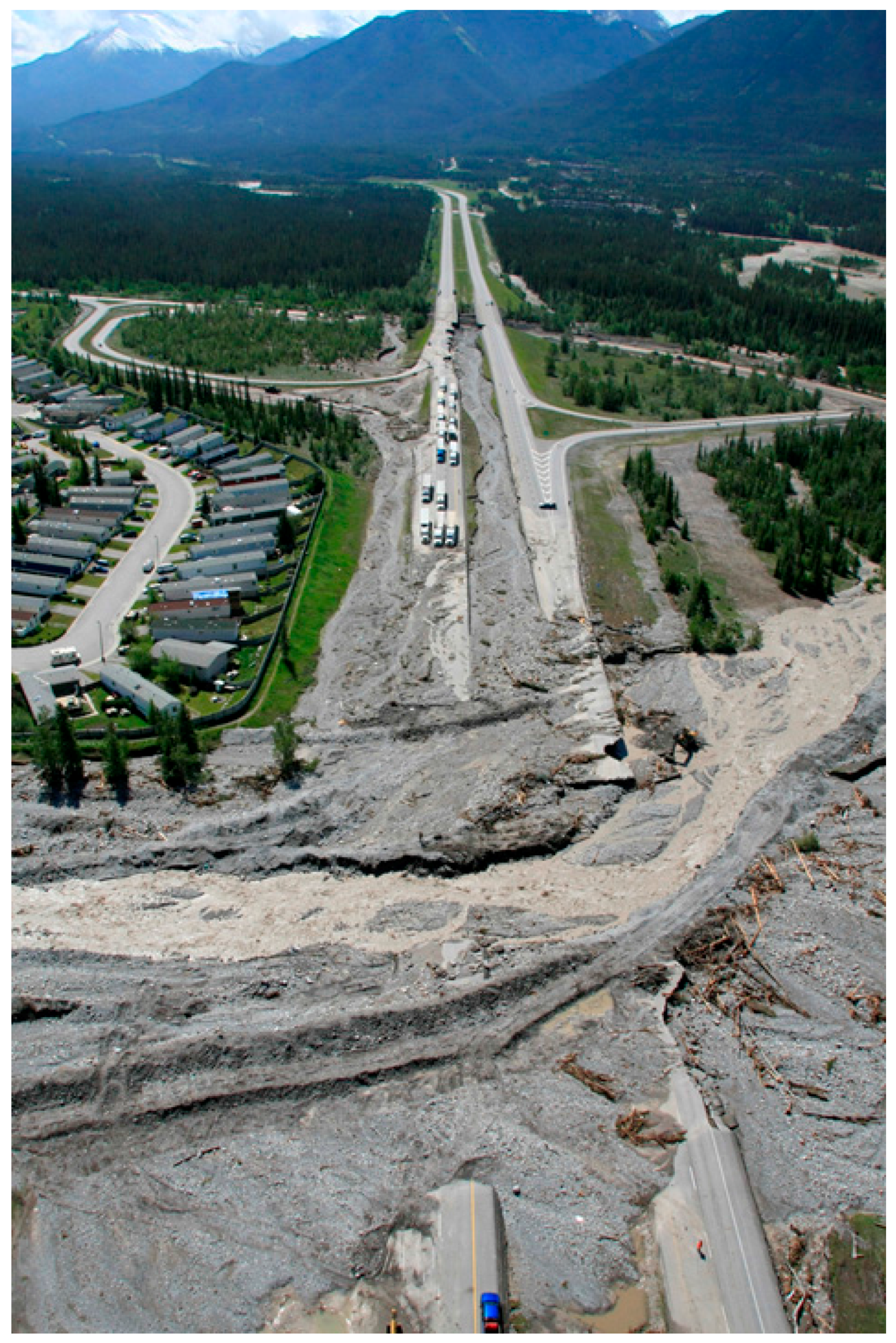
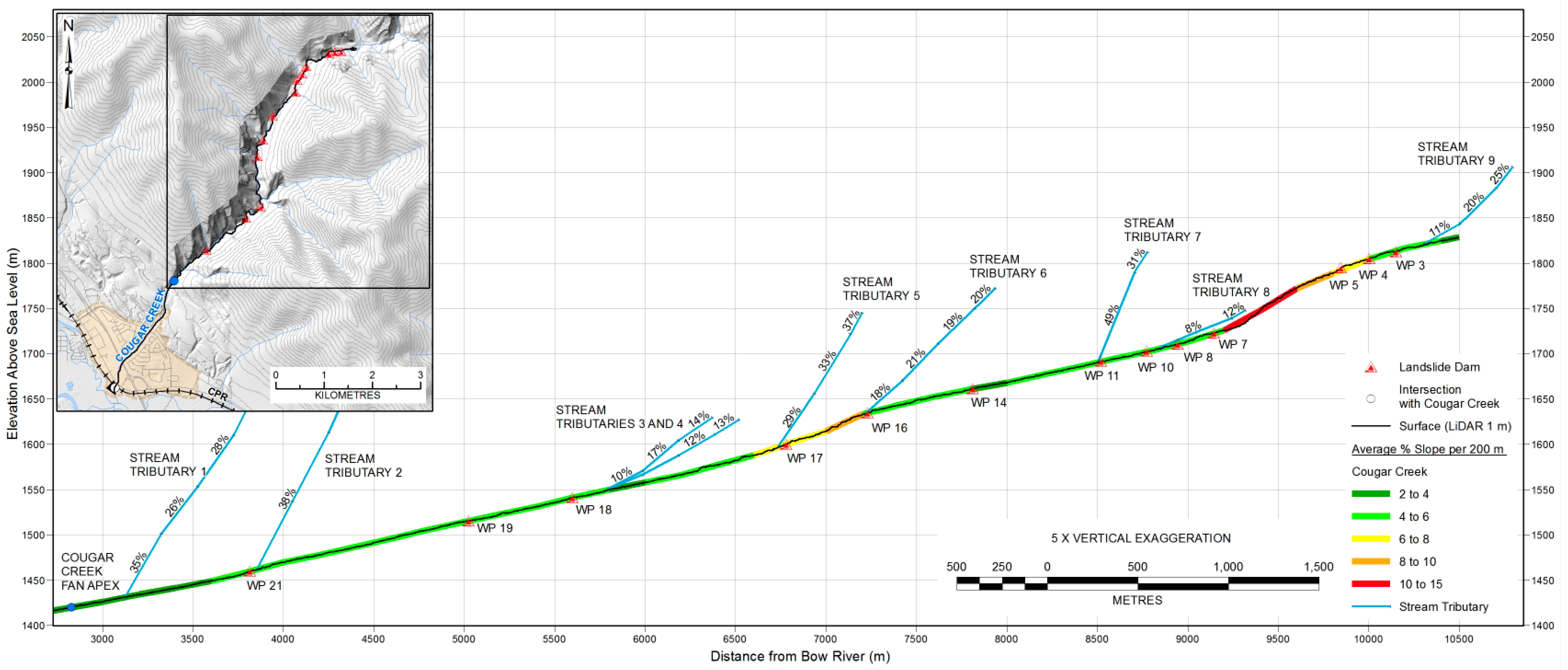
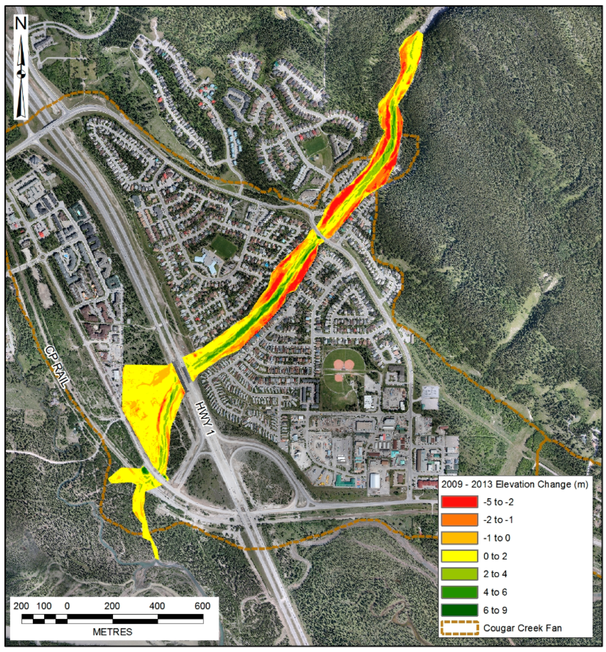
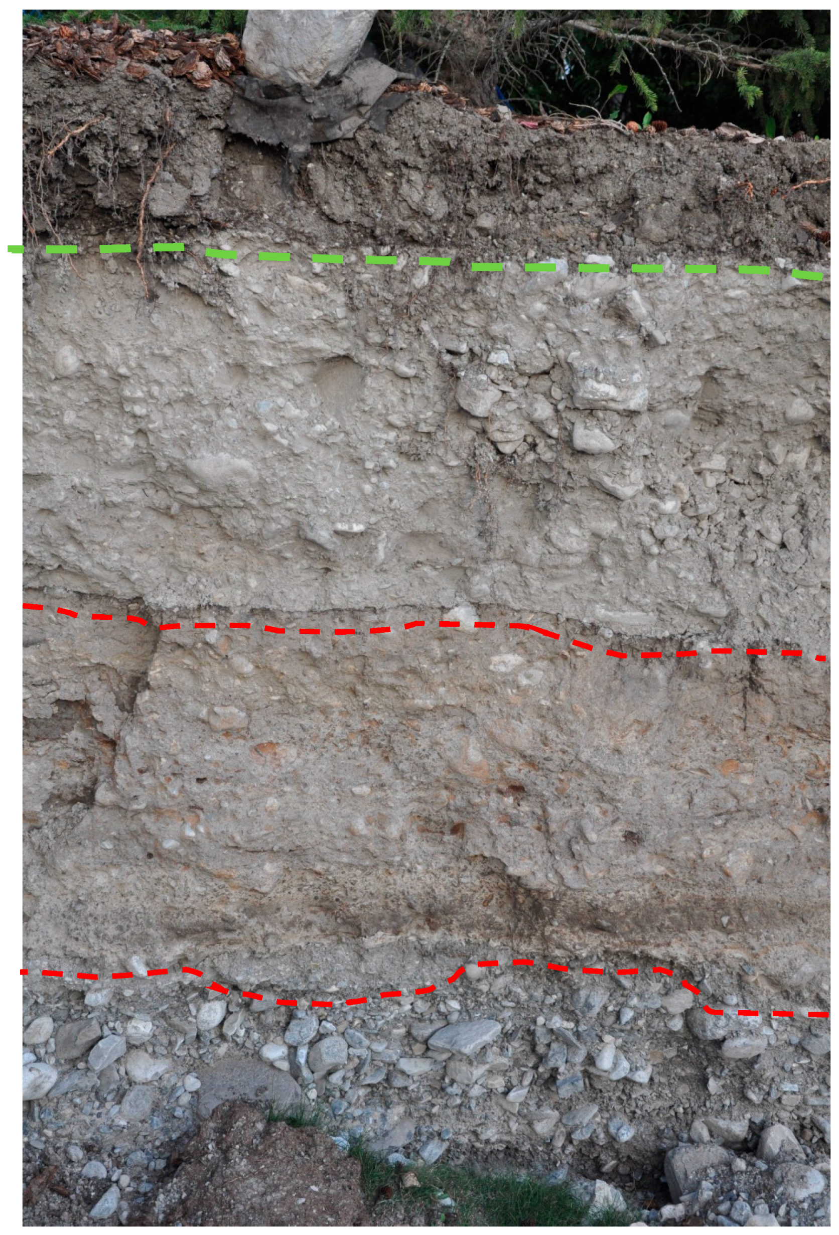
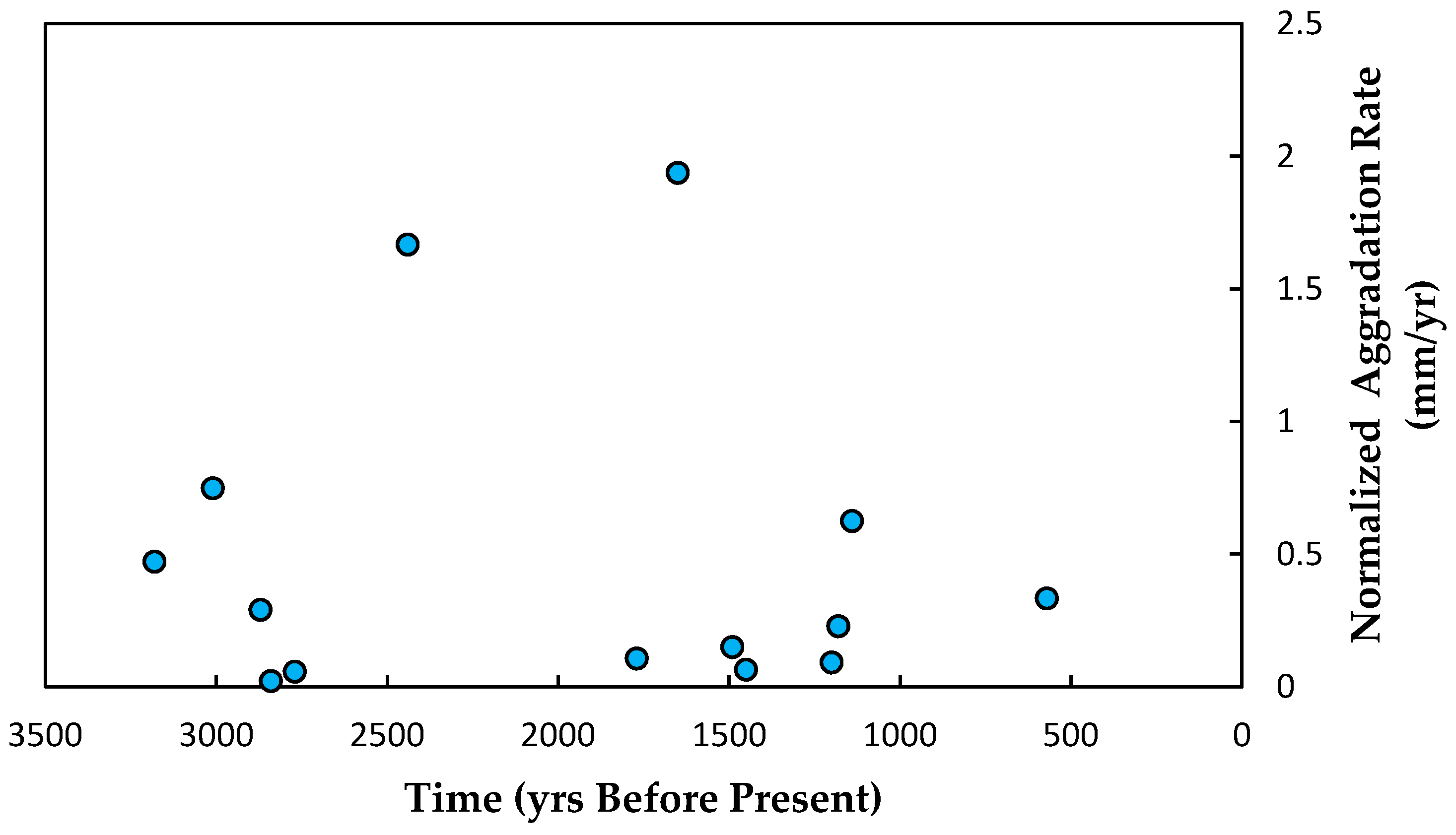
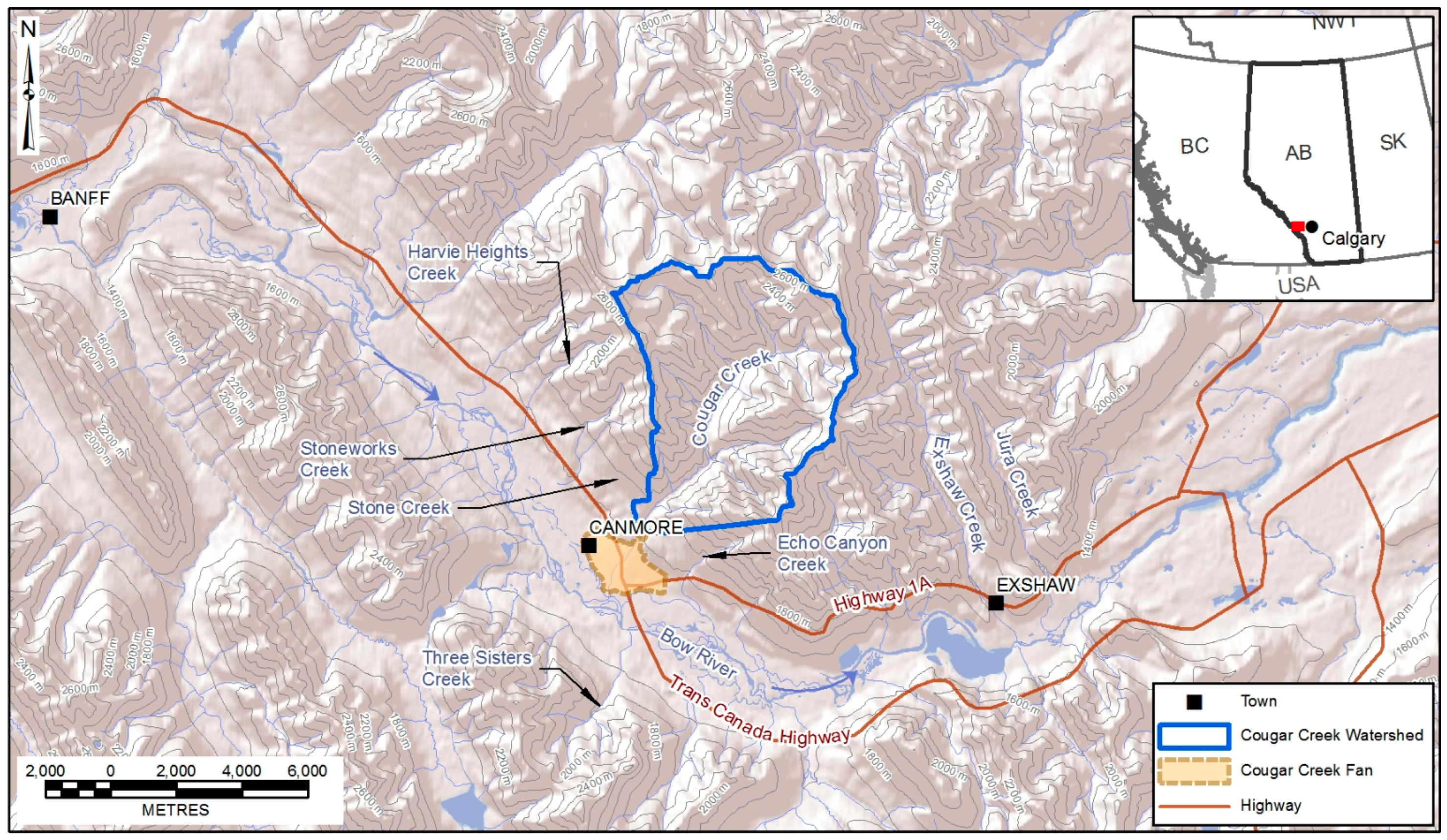
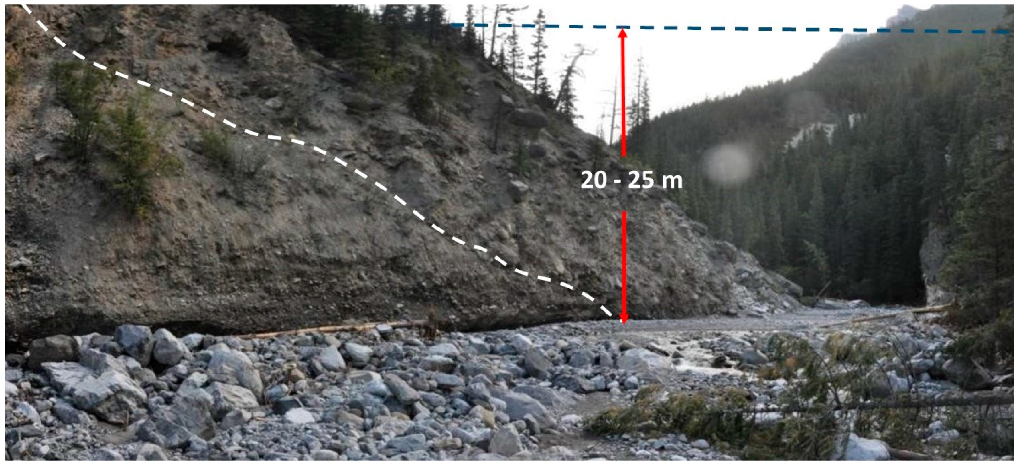
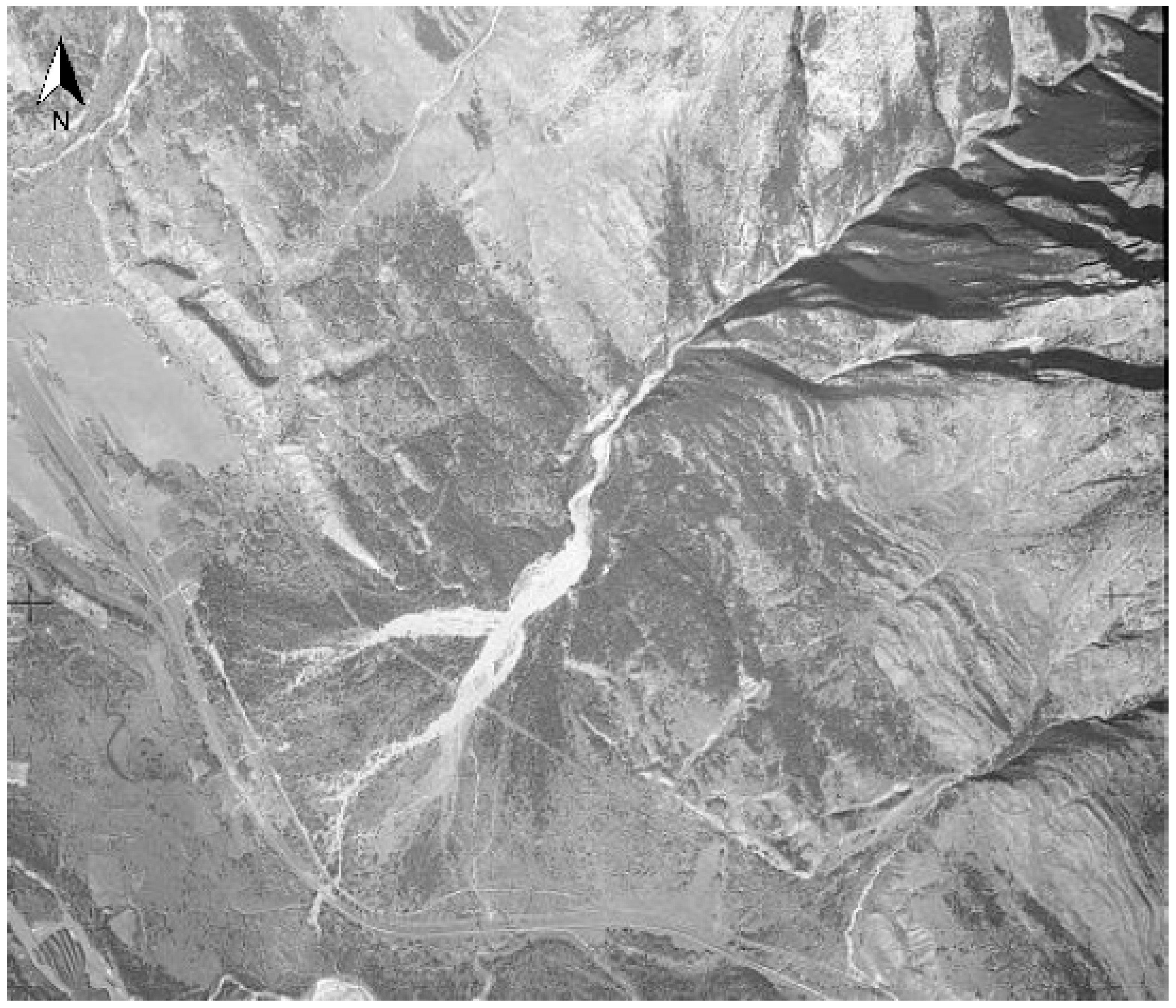
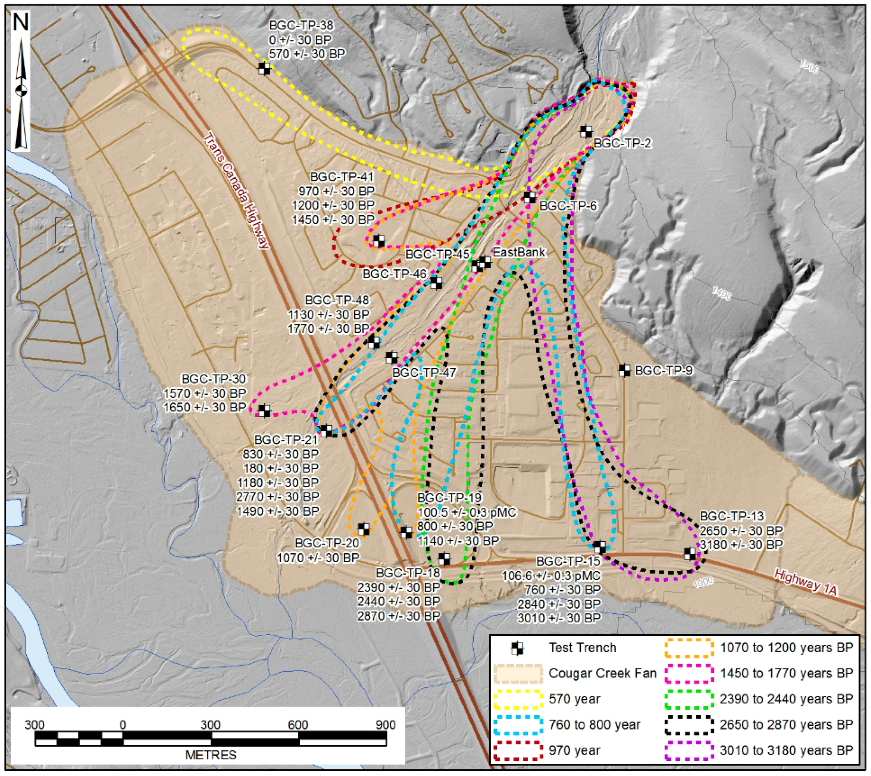
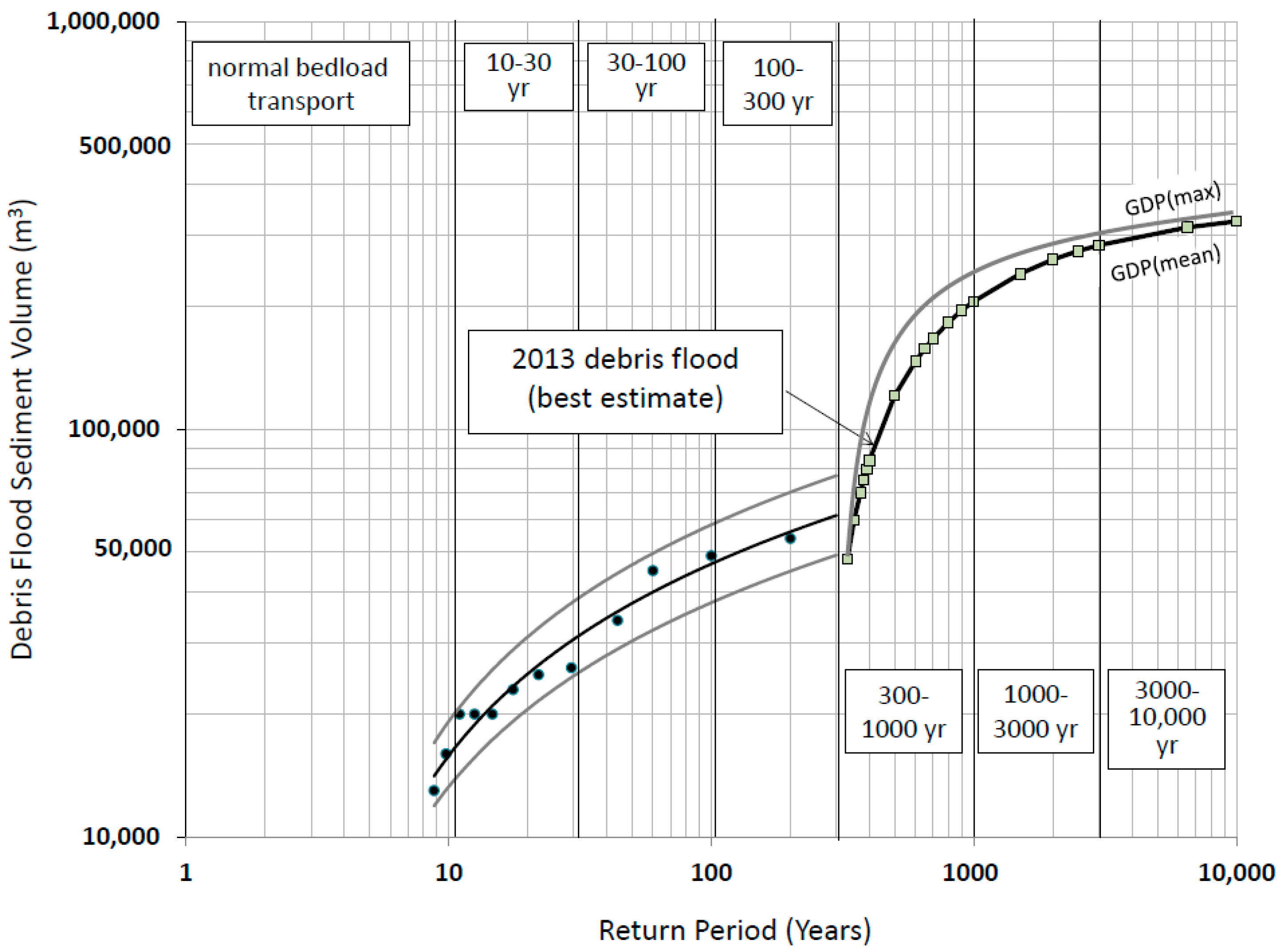