Assessment of Changes in Flood Frequency Due to the Effects of Climate Change: Implications for Engineering Design

Abstract

The authors explore the uncertainty implied in the estimation of changes in flood frequency due to climate change at the basins of the Cedar River and Skunk River in Iowa, United States. The study focuses on the influence of climate change on the 100-year flood, used broadly as a reference flow for civil engineering design. Downscaled rainfall projections between 1960–2099 were used as forcing into a hydrological model for producing discharge projections at locations intersecting vulnerable transportation infrastructure. The annual maxima of the discharge projections were used to conduct flood frequency analyses over the periods 1960–2009 and 1960–2099. The analysis of the period 1960–2009 is a good predictor of the observed flood values for return periods between 2 and 200 years in the studied basins. The findings show that projected flood values could increase significantly in both basins. Between 2009 and 2099, 100-year flood could increase between 47% and 52% in Cedar River, and between 25% and 34% in South Skunk River. The study supports a recommendation for assessing vulnerability of infrastructure to climate change, and implementation of better resiliency and hydraulic design practices. It is recommended that engineers update existing design standards to account for climate change by using the upper-limit confidence interval of the flood frequency analyses that are currently in place.

1. Introduction

Climate change can increase the likelihood of occurrence and strength of extreme weather such as extreme precipitation events [1], which might lead to cause more flooding in some regions. Changes in the frequency and intensity of flooding events may produce serious impacts on society, such as enormous economic, societal and environmental damage, including loss of lives. There were 539,811 deaths (range: 510,941 to 568,680), 361,974 injuries and 2,821,895,005 people affected by floods between 1980 and 2009 [2]. Many of the economic impacts of flooding are related to the damage on civil engineering infrastructure. There is a growing interest in learning about the impact of climate change on the engineering design of structures like bridges and culverts that are sited at the outlet of small and medium watersheds. According to projections, climate change is likely to concentrate rainfall into more intense storms [3,4,5]. Heavy rains can result in flooding, which could disrupt traffic, delay construction activities, and weaken or wash out the soil and culverts that support roads, tunnels, and bridges. For road transport infrastructures, weather stresses might represent from 30% to 50% of current road maintenance costs in Europe [6]. About 10% of these costs are associated with extreme weather events alone, in which extreme heavy rainfalls & floods events represent the first contribution. Traffic disrupted by flooding also has consequences in loss of lives. The primary cause of flood-related mortality in developed countries is drowning being in a motor-vehicle [2]. In the United States and other countries, civil engineers typically refer to historical data when designing hydraulic structures and transportation systems. For example, bridges are often designed to withstand storms that have a probability of occurrence of 1% every year, i.e., the 100-year return period flood [3].

Several authors have reported that the frequency and magnitude of important flows are being affected by the changes in climate conditions, land use and land cover among other factors [7,8,9,10]. [11] found that the frequency of 100-year return period floods increased substantially during the twentieth century in basins larger than 200 thousand square kilometers all around the world, and that there is a statistically significant positive trend in risk of great floods. These findings in the literature support the importance of taking into account the impacts of the climate change in the assessment of flood frequencies from river discharge projections.

Two approaches are found commonly in the literature to address this problem. The first is based on creating projections of discharge and/or flood frequency values based on observations from the past by means of statistical models [12]. The second approach is based on modeling the physical processes involved in the conversion from rainfall into runoff. In the latter, the assessment of changes in discharge projections is implicitly accounted by forcing a hydrologic model with rainfall projections that consider climate change. This approach, however, has some limitations. Using rainfall projections with coarse spatial and temporal resolution provided by General Circulation Models (GCM) might be sufficient for analyzing river discharge changes on a global scale [8,13,14,15,16], but it is not satisfactory for analyzing changes at smaller and medium size basins (100 to 10,000 km²). To provide meaningful results at small or medium basin scales, it is necessary to produce rainfall projections with adequate spatial and temporal scales that can be used as forcing in fine resolution hydrologic models [17,18,19,20].

The process of downscaling rainfall projections at higher spatial and temporal scales has an inherent uncertainty. That uncertainty propagates through the chain of processes required for transforming rainfall projections to peak flow discharge estimates. Additionally, other sources of uncertainty need to be taken into account. These include: the uncertainty of the hydrological model; the uncertainty of each climate model to reproduce the projections of precipitation; the dispersion among the projections from different climate models; the uncertainty on the emission scenarios in the climate models; and the uncertainty of the flood frequency assessment which arises from the fitting procedure, and the assumptions about the statistical distribution to be used. Further, the accuracy of procedures is challenged by the uncertainty related to future changes of additional factors affecting hydrologic simulation, such as evapotranspiration and land use. All these sources of error produce considerable uncertainty that must be taken into account, but their individual study is out of the scope of this paper. The authors aim to focus on factors where more uncertainty relies, considering the errors of climate models projections [21,22] and the flood frequency analysis procedure [23]. Sensitivity to hydrologic model parameterization is important, but not addressed in this paper, considering that most of the contribution to total uncertainty comes from the model inputs [24]. The study accounts for the uncertainty in the flood frequency assessment and evaluates the sensitivity to the assumption of stationarity, length of data series, and the spatio-temporal resolution of the downscaled rainfall data.

The authors attempt to assess the expected changes in the frequency of floods in two watersheds in Iowa due to climate change. Rainfall projections obtained from 19 climate models in a region that includes Iowa were forced into a distributed hydrological model to produce discharge projections. The setup of the experiment requires taking into account special considerations for providing meaningful results at the desired spatial and temporal scales. For that purpose, the used rainfall projections are downscaled in both spatial and temporal scales using an algorithm capable of reproducing the tails of historical daily precipitation distribution with relatively low sensitivity to non-stationarity in climate model projections of precipitation [25,26,27]. Next, flood frequency analysis of the hydrologic model generated data was made using the software Peak Flow Frequency (PeakFQ) [28], the software adopted by United States Geological Survey (USGS) to provide flood magnitudes and their corresponding variance, using the log-Pearson Type III frequency distribution. The approach implies assuming stationarity of discharge projections, following the guidelines for determining flood flow frequency reported by USGS in the Bulletin 17B [29]. In Section 2 is described the data and the area of study. Section 3 describes the applied methodology. Section 4 presents the results, and Section 5 summarizes the conclusions and discussion.

2. Study Area and Data

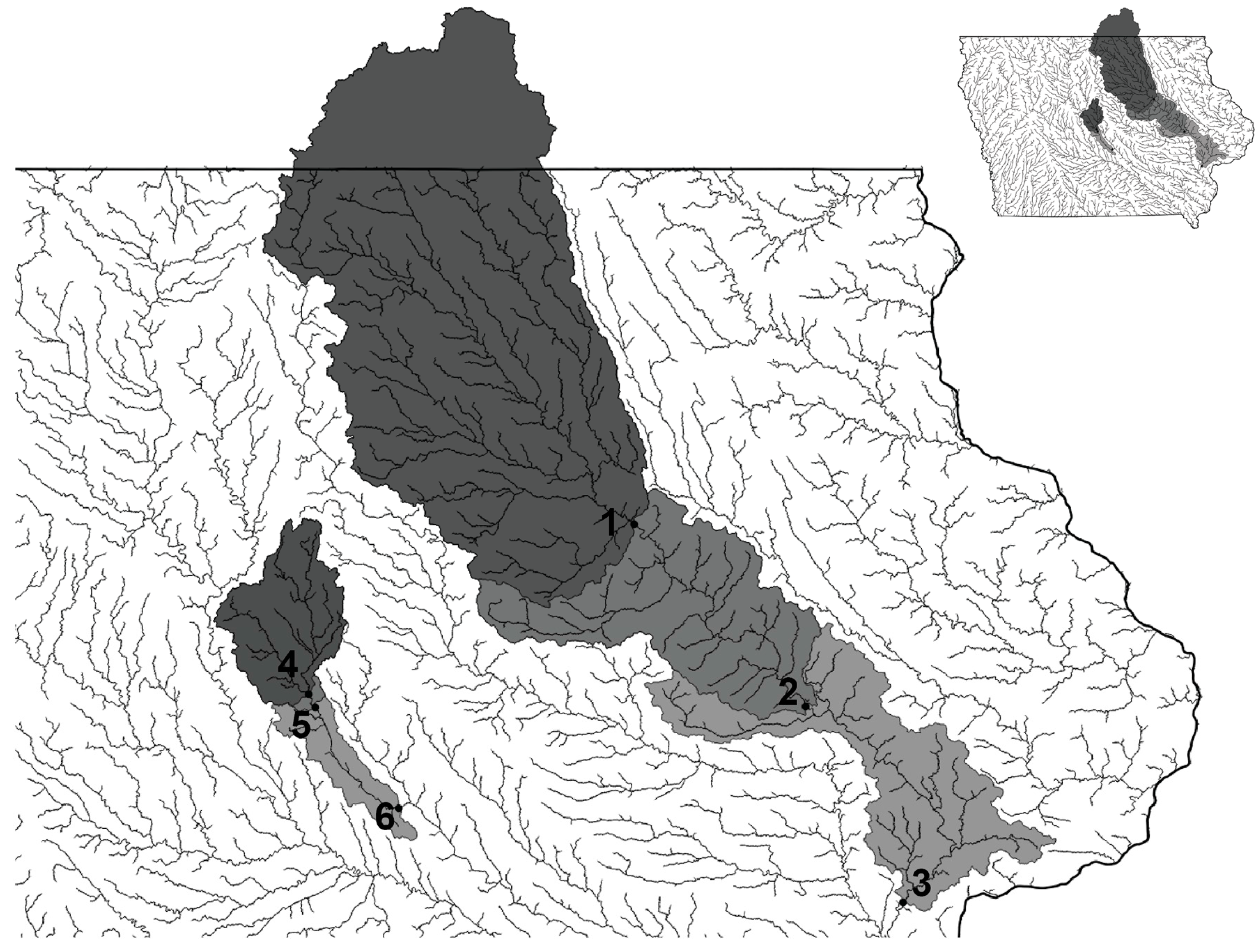
2.1. Selected Basins and Observed Streamflow

The study area is the South Skunk River Basin in Central Iowa and the Cedar River Basin in Northeast Iowa (see Figure 1). Within these basins, six locations were selected where the river intersect major interstate highways and passes under a bridge. The three bridges along the Cedar River are collocated with United States Geological Survey (USGS) gauges where historical streamflow observations are available. The bridges of the South Skunk river also have collocated USGS gauges, except for the bridge marked with number 5 in Figure 1, which is just a few kilometers downstream of bridge number 4.

Table 1. Bridge locations and available stream gauges.

Map (No.) *	Bridge Location	USGS Gauge (No.)	Drainage Area of Gauge (km2)
1	Cedar River: US 20 in Waterloo	05464000	13,294
2	Cedar River: US 151 in Cedar Rapids	05464500	16,814
3	Cedar River: I-80 near West Branch	05465000	20,080
4	Skunk River: US 30 in Ames	05471000	1458
5	Skunk River: I-35 south of Ames	05471000	1458
6	Skunk River: I-80 in Colfax	05471050	2105

* Corresponds to numbered locations in Figure 1 map.

summarizes the information about the location of the bridges, the available streamflow gauges and their upstream areas.

2.2. Rainfall Data Sets

The study uses the precipitation of climate projections from the High-Resolution National Climate Change Dataset [26]. The database consists of daily projections from 1960 to 2099 from global models archived by the Coupled Model Intercomparison Project version 3 (CMIP3) [30]. The projections are simulations from multiple climate models of multiple future greenhouse gas concentration scenarios, which are summarized in

Table 2. Global climate modeling groups and their models. Source: High-Resolution National Climate Change Dataset. Those marked with * begin in 1961. All other models contain daily time series from 1960 to 2099.

Origin	CMIP3 Model	Scenarios
National Center for Atmospheric Research	CCSM3	A1FI, A2
Canadian Centre for Climate Modelling and Analysis	CGCM3.1-T47 * CGCM3.1-T63 *	A2, A1B A2, A1B
Centre National de Recerches Meteorologiques	CNRM-CM3	A2, A1B
Max Planck Institute for Meteorology	ECHAM5	A2, A1B
National Institute for Meteorological Research/Korea Meteorological Administration	ECHO-G	A2, A1B
NOAA Geophysical Fluid Dynamics Laboratory	GFDL–CM2.1	A2, A1FI
UK Meteorological Office Hadley Centre	HADCM3 HADGEM1	A1FI, A2, A1B A2, A1B

. The native grid of climate projection data ranges from 1-degree to 2.5-degrees latitude by longitude, which is too coarse to represent rainfall within basins that range from 500 to 20,000 km² in this evaluation. The models were downscaled using the asynchronous regional regression model (ARRM, [25,26]), resulting in a spatial partitioning of 1/8-degree cells and temporal daily increments. Unfortunately, CMIP5 downscaled data was not available when our research was conducted.

Because frequent practice with the hydrology model used in this study is to use rainfall estimates with 4-km cells and hourly increment, there were designed a series of data degradation experiments, starting from Stage IV radar rainfall [31], to show the sensitivity of hydrological simulation for flood prediction to data coarseness. The experiments are detailed in Section 3.

3. Methodology

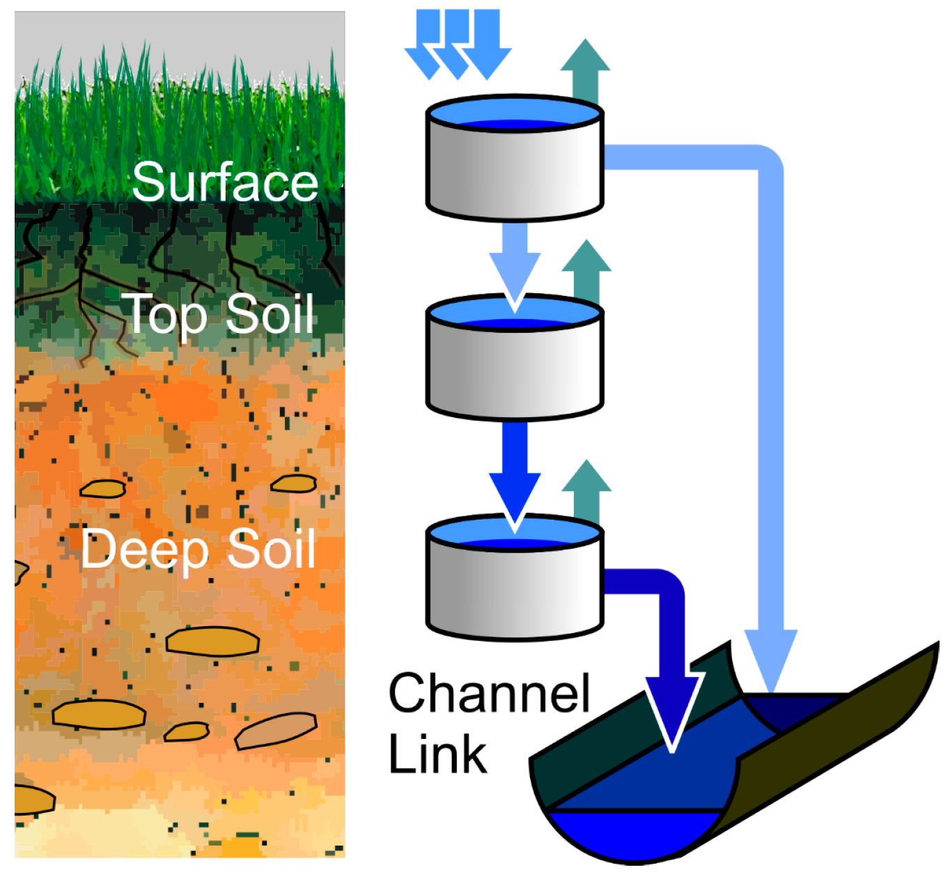
3.1. Distributed Hydrological Model

The Hillslope-Link model (HLM) distributed model [32,33] was used to transform the rainfall from the climate projections into discharge simulations. For the setup of the experiments, it is assumed that there are not changes in projections of evapotranspiration and land use. HLM builds on the concept of the landscape decomposition into hillslopes and channels [34]. HLM allows for flexible structure and the representation of the physical processes of runoff generation and water transport; the processes include initial abstraction, infiltration, overland flow, percolation, base flow, and channel routing. HLM is calibration free, i.e., a common configuration of parameters determined a priori applies to all the hillslopes. Each hillslope contains four water storage components (see Figure 2): channel storage, water ponded on hillslope surface, effective water depth in the top soil layer, and effective water depth in hillslope subsurface. The mass conservation equations of the water storage are defined in terms of ordinary differential equations. Channel streamflow is contributed by several flow components: (1) overland flow from the water ponded on hillslope surface; (2) interflow from the water depth in the top soil layer; and (3) baseflow from the hillslope subsurface. The mass transport for each channel link in the network is defined as a power law relation that describes flow velocity as a function of discharge and drainage area [35]. HLM has been used extensively as the backbone of the operational flood forecasting system used by the Iowa Flood Information System IFIS [32]. More details about the HLM equations, configuration, and numerical solver are provided in [33] and [32]. Examples of HLM applications are provided in [32,33,36,37,38,39,40,41,42,43].

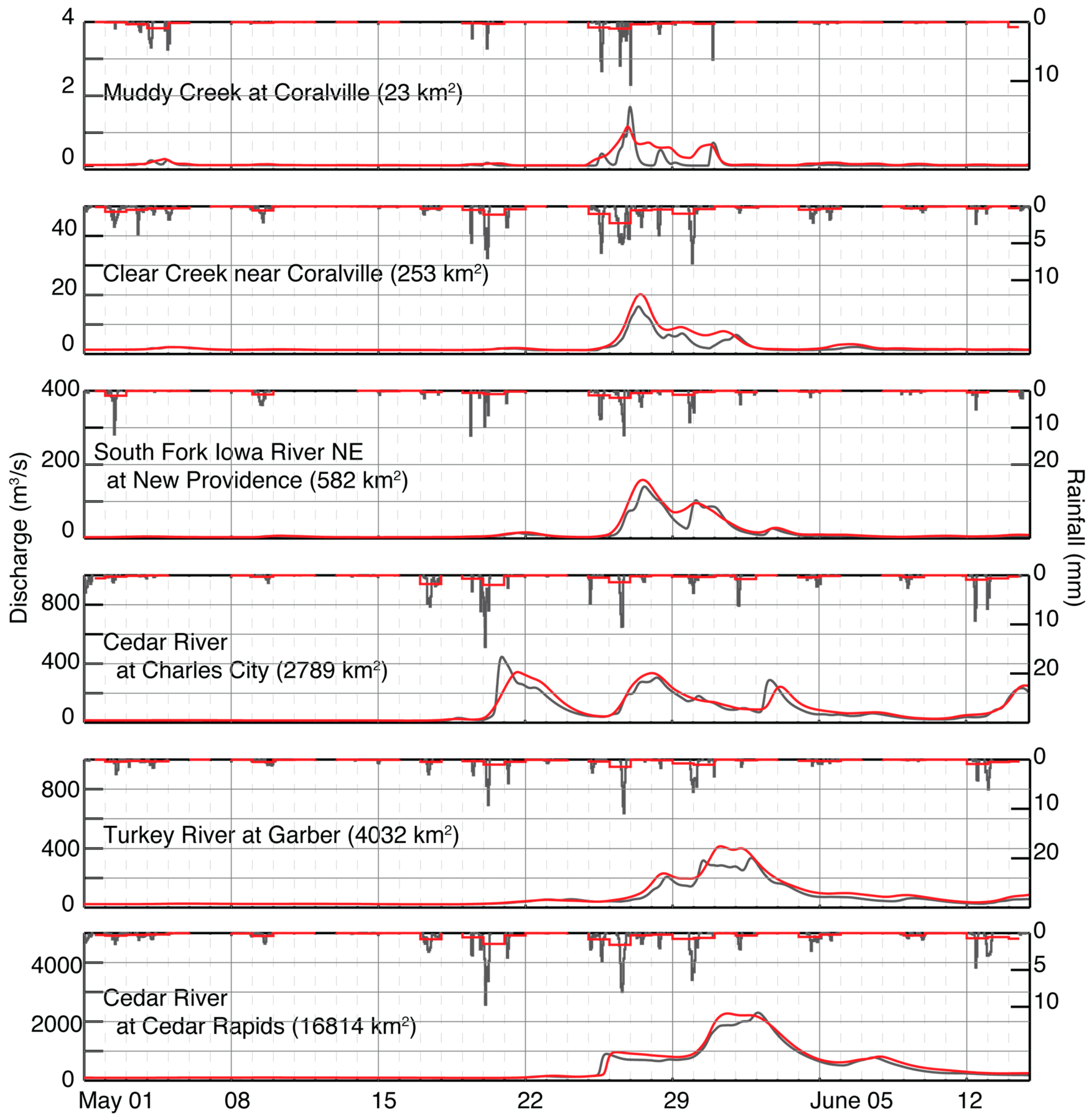
3.2. Model Sensitivity to Spatial and Temporal Resolution of Rainfall Datasets

The use of rainfall with 1/8th degree cells and daily increment may be inadequate for assessment of peak flows in small and medium watersheds. Coarse spatial and temporal scale of rainfall may distribute rainfall with unrealistic evenness across watersheds and may result in underestimation of peak flow values [40]. It was developed a data degradation experiment to test for this possibility. If forcing coarsened precipitation data into the model resulted in poor peak flow simulation, it would conclude the resolution of the climate projection data set is inadequate. Peak flows were estimated at catchments of multiple spatial scales, first by forcing our hydrologic model with Stage IV radar rainfall estimates at the native scales of ~4 km cells with hourly increment. Subsequently the Stage IV resolution was degraded to daily accumulation on 1/8th degree cells. Figure 3 shows the differences in the resulting hydrographs at six catchments in Iowa with different upstream areas. The basins are sorted by upstream area. Results are shown for a period of intense rainfall events that occurred in the spring of 2013 in Eastern Iowa. The hydrographs produced with native Stage IV data are shown as gray lines and the ones produced with daily-1/8th degree degraded Stage IV data are shown as red lines. In terms of the assessment of peak flows, the magnitude of the differences seems to be related with the spatial scale of the basin. The smallest basin considered has an upstream area in the order of tenths of square kilometers, and approximately a −35% difference in the peak assessment. Peak differences diminish as upstream area increases. The upstream area of the largest basin considered is in the order of tenths of thousands square kilometers, and the difference in peak assessment is approximately +5%. The authors acknowledge that is hard to make strong conclusions based on the results of few basins in a short time period of analysis. The basins of study in the Cedar River and Skunk River have upstream areas in the order of thousands and tens of thousands square kilometers (see Table 1). The results of the degradation experiment show empirical evidence that the limitations on resolution of rainfall projections will not affect significantly the estimation in the magnitude peak flows on discharge projections for these basins.

3.3. Flood Projections Estimates

The model simulations consist of 19 continuous daily discharge time series derived from each rainfall projection for each site. The series are analyzed in the period between 1 January 1960 and 31 December 2099. An exception is made for the CGCM3 model, which starts in 1 January 1961. For every year, were produced simulations starting 1 April and ending 1 December, in order to model only the warm season of the year. Modeling these months avoids the problems caused by precipitation estimation during the winter and the inability of HLM to simulate snowmelt processes. The model produced hydrographs at every location of the drainage network of Iowa. The hydrographs obtained at the six catchments are analyzed in the results section.

3.4. Flood Frequency Analysis

The annual peaks were extracted from the 19 daily discharge time series simulated by the hydrologic model. The resulting 19 series of simulated annual maxima were used for performing flood frequency analysis. The software PeakFQ [28] was used to estimate the discharge of different return periods, including the 100-yr flood, as used traditionally in bridge design. Two time periods were selected to perform the flood frequency analysis with PeakFQ. The first period includes simulated annual peaks between 1960 and 2009. This date range is selected with the aim of performing a validation of the methodology using observed peaks at USGS gauges. Table 1 shows the available observed discharge data from the gauges. The flood frequency analysis was extended to the observed annual peaks and compared with the peaks derived from the simulations in the same period. In the second period, was taken the whole range of projected discharges, between 1960 and 2099. The findings of the second period analysis were compared with the results of the first period in order to illustrate the expected changes in the projections between 2009 and 2099.

3.5. Sensitivity of Flood Frequency Analysis to Selected Period of Analysis and Record Length

It is standard procedure to use all available historical data in flood frequency estimation; however, a standard procedure has not been established for projections of future periods. The study evaluated also the sensitivity of the flood frequency analysis to length of period of analysis. Two experiments were conducted to explore the sensitivity of flood frequency estimation based on the amount of available data that is used as input into PeakFQ. In the first experiment, PeakFQ was fed with data over a growing time window, starting with the period 1960–1999 and increasing the upper limit with increments of one year (i.e., 1960–2000, 1960–2001, and so on) until the window covered the period 1960–2099. Every time the window is expanded, were obtained the 100-yr flood and its 95% confidence intervals. In the second experiment, PeakFQ was fed with data over a 40-year period, starting with the period 1960–1999. Subsequently, the 40-year window was moved forward in increments of one year (i.e., 1961–2000, 1962–2001, and so on), until the window reaches the period 2060–2099. For every time window were obtained the 100-yr flood and its 95% confidence intervals. The size of the time window is subjective. It was considered 40 years because it is a common value of data availability. The results of this analysis are presented in Section 4.3.

4. Results

Here are presented the detailed results of our methodology in the catchment of the Cedar River at Cedar Rapids (~16,840 km²), and then a summary of the findings at the six catchments selected in this study.

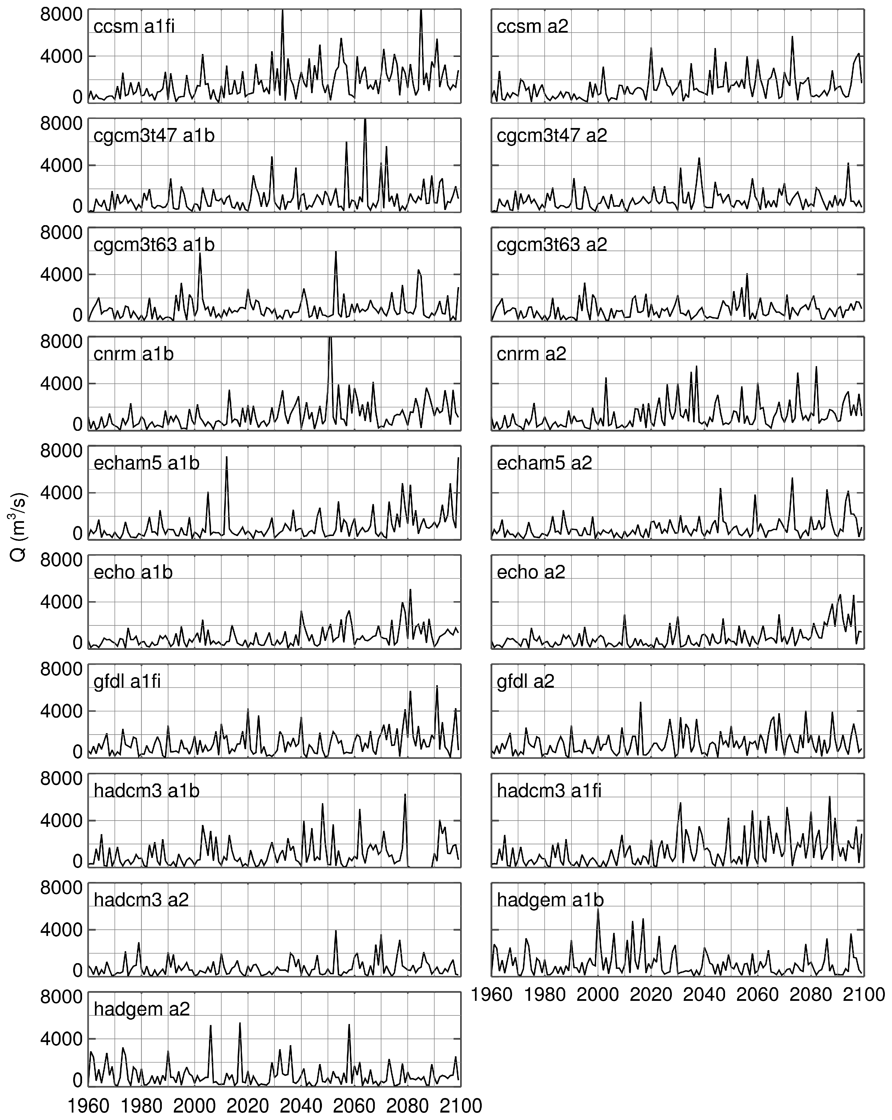
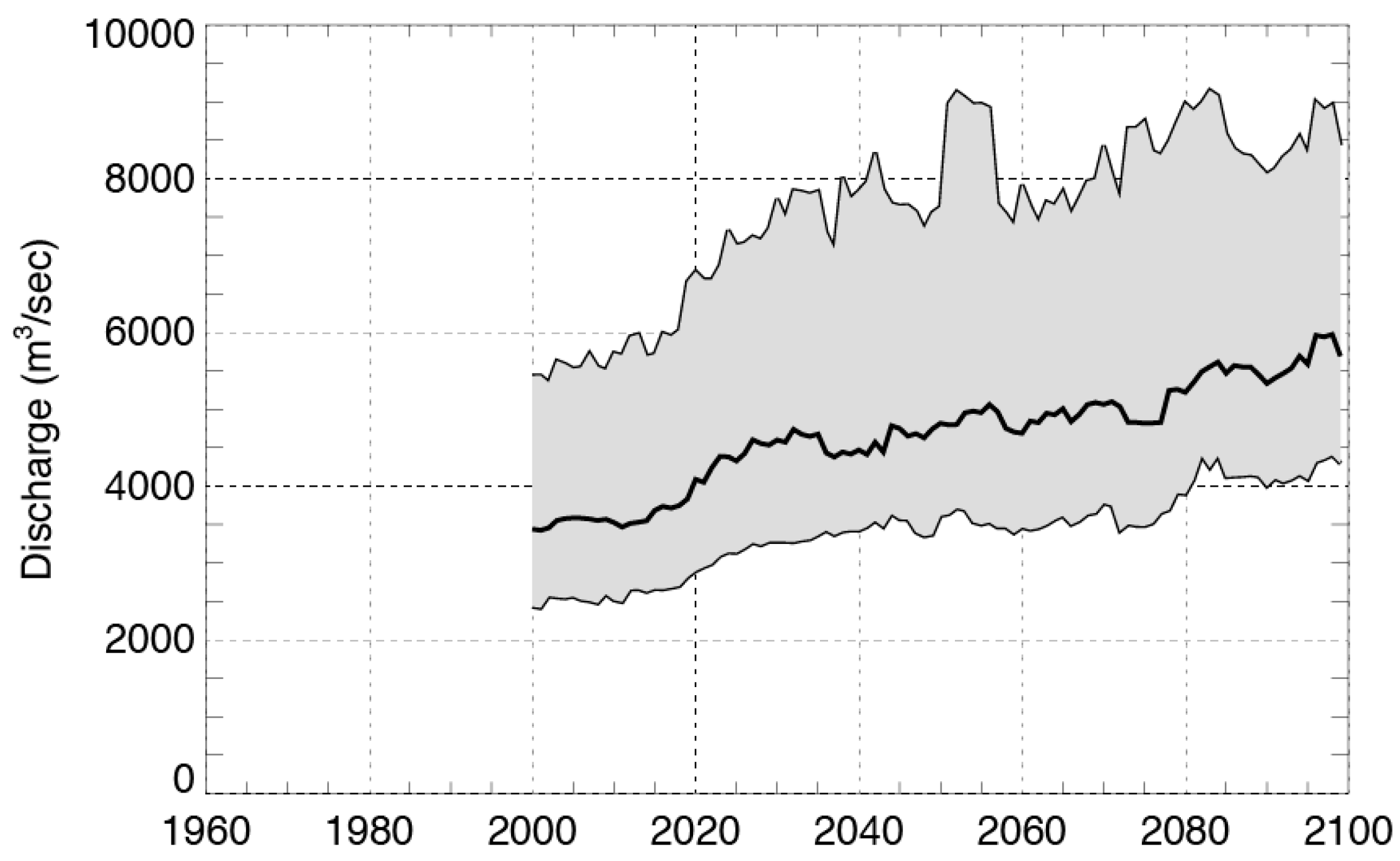
4.1. Projected Annual Peak Flows and Trends

Figure 4 shows the time series of annual peak flows obtained for the catchment of Cedar River at Cedar Rapids for each of the climate projections, organized by models and scenarios. One can see that the magnitude of the projected annual peaks varies in different ways for every projection. The annual peaks simulated with the hydrologic model when forced with the rainfall projections from CCSM A1FI, CGCM3T47 A1B and CNRM A1B models reach values of up to 8000 m³/s. These peaks would correspond to flood values with a return period greater than 500 years when compared to historical observations [44].

The Mann-Kendall non-parametric trend test [45,46] was used to detect significant trends in the mean of annual peak flows at the 5% significance level. The calculations were performed using the Kendall package in R [47]. The results of the Mann-Kendall test over the 19 annual peak time series are summarized in

Table 3. Parameters obtained after a Mann-Kendall test with alpha = 0.05 for detection of trends in the projected annual peak flows in the bridge of US 151 in Cedar River at Cedar Rapids.

Model and Scenario	Mann-Kendall’s Tau	p-Value	p-Value < 0.05
CCSM A1FI	0.278	1.07 × 10−6	true
CCSM A2	0.273	1.79 × 10−6	true
CGCM3T47 A1B	0.129	0.024	true
CGCM3T47 A2	0.183	0.0013	true
CGCM3T63 A1B	0.031	0.58	false
CGCM3T63 A2	0.095	0.095	true
CNRM A1B	0.300	1.19 × 10−7	true
CNRM A2	0.242	2.37 × 10−5	true
ECHAM5 A1B	0.131	0.021	true
ECHAM5 A2	0.205	0.00033	true
ECHO A1B	0.124	0.029	true
ECHO A2	0.059	0.30	false
GFDL A1FI	0.053	0.35	false
GFDL A2	0.120	0.035	true
HADCM3 A1B	0.091	0.11	false
HADCM3 A1FI	0.224	9.18 × 10−5	true
HADCM3 A2	−0.003	0.96	false
HADGEM A1B	−0.017	0.77	false
HADGEM A2	−0.017	0.77	false

. It shows the tau and p values obtained for each model. In seven out of 19 models, the results show evidence to reject the null hypothesis H₀ of no monotonic trend in the time series at the 5% significance level. However, this statistical evidence of trend in the mean of the annual peaks appears mostly for the results of the Hadley Centre model (four out of seven), which suggest that their climate model produce more extreme rainfall values compared to other models.

In this study, it was assumed that the process of translating 19 climate model rainfall projections into discharge projections is stationary, and then the methodology proposed in Bulletin 17B can be applied to perform flood frequency analysis. The authors acknowledge that a more comprehensive study should consider an approach for flood frequency estimation for nonstationary processes, and that results can be severely affected (see [48,49] for additional discussion in this topic). For the purposes of this study, our assumption reveals results from a pragmatic perspective, which follows the guidelines of traditional engineering practice.

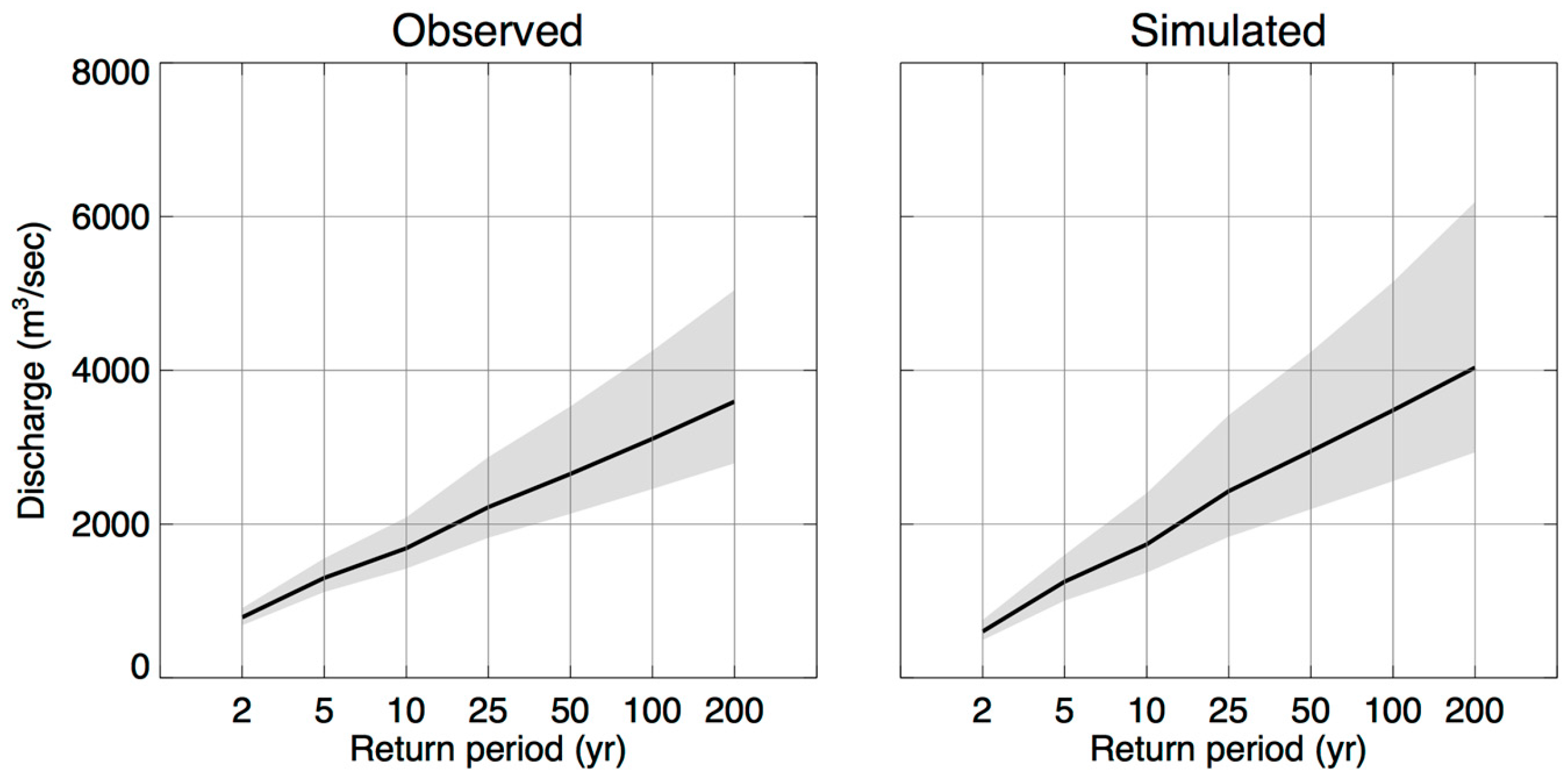
4.2. Projected Floods for Different Return Periods

The series of projected annual peak flows were used to run a flood frequency analysis using PeakFQ. These analyses generated 19 different values (one for each climate model) of the estimated discharge for the 2, 5, 10, 25, 50, 100 and 200-year return periods, including their 95% confidence intervals. The methodology was validated by comparing the flood frequency analyses of the projected discharge from 1960 to 2009 and the annual peak values observed at the corresponding USGS station in the same period. The period 1960 to 2009 was picked up with the purpose of using at least 50 years of observed data for the validation of the methodology. Figure 5 shows the results of the validation analysis. The figure in the right panel compiles the results obtained with the 19 climate projections by plotting the median of the discharge values for different return periods and the median of the confidence intervals. The election of using the median to summarize the magnitude of the discharge values and the confidence intervals is made to provide simplicity to the comparison of observations and simulations and as a means to communicate a representative value of the discharge projections. The values of the simulated discharges are in the same order of magnitude to the observed flood values, especially for the lower return periods. As stated previously, the authors do not aim to obtain exact values with the simulations, but expect these to be in the same order of magnitude of the flood frequency values derived from observations. These observations are also subject to a lot of uncertainty due to the limited record length, especially for large return periods. The envelope of the 95% confidence interval of the flood estimator is given in the gray shaded area. The envelope of the simulations ensemble contains the envelope of the observational uncertainty. The historical observations are contained by possible realizations of the models. From the previous result, it will be assumed that the simulations for the period 1960–2009 are a valid predictor of the observed flood frequencies on that period.

A second set of data analysis addresses the question of how the flood frequencies will change between 2009 and the end of the 21st century. In some manner, this experiment addresses the question of what is the change in flood frequency values from present time to future in the basins of the Cedar and South Skunk River. For that purpose, were assessed the flood frequencies of the year 2099 by analyzing the data in the period 1960–2099 and compare those to the frequencies derived for 1960–2009. Figure 6 compares the distribution of flood frequencies in the period 1960–2009 derived from model simulations (solid black line is the median and gray envelope are the 5–95% confidence intervals) with the distribution of flood frequencies in the period 1960–2099 (solid blue line is the median and dashed blue lines are the 5–95% confidence intervals). Figure shows that by the end of the 21st century, there could be an increase in the magnitude of the flow values of all the return periods, as well as for the confidence intervals of these estimates. According to these results, the median of the flood frequencies by the year 2099 will be very similar to the upper confidence interval of the flood frequency values in the present period. This particular result is interesting from an engineering design perspective, since it provides some guidance about how in present time, policy makers could incorporate consideration of climate change in regulations for design, by using the upper limit confidence interval of the current flood frequency analyses as an updated, climate-change-ready design standard.

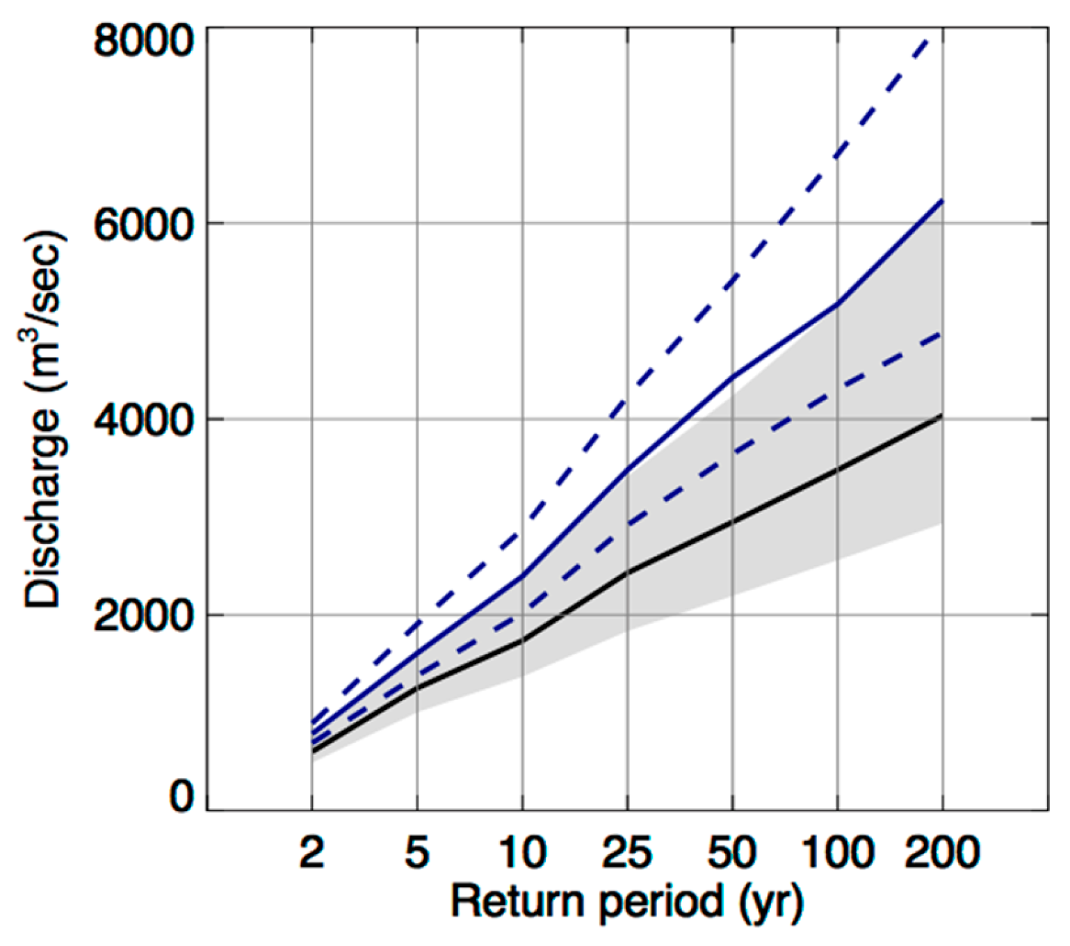
4.3. Changes in the 100-yr Flood Estimates and Their Sensitivity to Availability of Information

It is of particular interest in this study to evaluate the results of the previous analysis for the 100-yr flood return period, given its importance in engineering design.

Table 4. Differences in the estimation of the 100-yr flood and their 95% confidence intervals over the periods 1960–2009 and 1960–2099 at the selected bridges.

100 yr-Flood (5%, Median, 95%)
Basin	1960–2009	1960–2099	Difference (%)
Cedar River: US 20 in Waterloo (05464000)	2378, 3219, 4884	4004, 4915, 6266	68, 52, 28
Cedar River: US 151 in Cedar Rapids (05464500)	2558, 3480, 5150	4306, 5173, 6705	68, 48, 30
Cedar River: I-80 near West Branch (05465000)	2607, 3514, 5218	4332, 5196, 6773	66, 47, 29
Skunk River: US 30 in Ames (05471000)	444, 635, 1019	652, 820, 1075	46, 29, 5
Skunk River: I-35 south of Ames (05471000)	466, 665, 1070	676, 836, 1105	44, 25, 3
Skunk River: I-80 in Colfax (05471050)	532, 738, 1168	793, 995, 1310	49, 34, 12

summarizes the changes that could experience the 100-yr flood between 2009 and 2099 at the six catchments of this study. The results show that the median of the 100-yr flood could increase between 47% and 52% in the catchments of the Cedar River, and between 25% and 34% for the South Skunk River. The upper and lower confidence intervals of these estimates could increase as well, as reported in Table 4. Although the results obtained at the Cedar River show an inverse relationship between the upstream area and the change in the median of the 100-yr flood, it would require this kind of analysis at basins of multiple scales to produce a statement about the relationship of these two variables.

In order to provide a context for the magnitude of the changes of the 100-yr flood it was performed a sensitivity analysis for the estimator with respect to the selected period of analysis and the record length. Additionally, it was studied the sensitivity of the 100-yr flood assessment to the amount of information that is used for its estimation.

In Figure 7 we calculated the 100-yr flood and their 95% confidence intervals for every year between 2000 and 2099, using a growing window, as described in Section 3.5. For example, for the year 2000, the 100-yr flood is estimated as the median of the 19 values of 100-yr flood estimates using data from 1960 to 1999 (40 years of data); in 2001 using data from 1960 to 2000 (41 years of data), etc. The 100-yr flood increases gradually, without exhibiting drastic changes, as new data is included for the analysis. The spread of the uncertainty envelopes remains more-or-less constant. Moreover, these envelopes could tend to be narrower as more data is used because the reduction of the standard deviation of the estimates.

The study also shows the sensitivity of the estimation of the 100-yr flood to the selected period of analysis by using portions of the available information. In Figure 8 was calculated the 100-yr flood and their 95% confidence intervals for every year between 2000 and 2099, using only the most recent 40 years of data, as described in the second experiment of Section 3.5. For example, for the year 2000, the 100-yr flood is estimated as the median of the 19 values of 100-yr flood estimates using data from 1960 to 1999; for 2001, using data from 1961 to 2000, etc. The same procedure is applied for the 5% and 95% confidence intervals. When using this approach, estimates are very sensitive to the extreme values contained in this relatively short amount of available data (40 years), and in consequence the metric sometimes exhibits large increases and decreases over the time, as well as their confidence intervals. This effect is especially notable between 2050 and 2055, where one can see how the peaks in the upper confidence intervals increases and decreases drastically in a short period of time.

5. Discussion

The aim of this study on hydrological climate change projections is to evaluate procedures for accuracy of data they produce, their strengths and weaknesses, and veracity of stated and unstated assumptions. The simulation data flow involves a series of simulation systems, each with their own assumptions and sensitivity to data input quality. The simulation chain starts with global climate model simulations-based upon multiple scenarios of future (unknowable) human greenhouse gas emissions, proceeds with a single downscaling method to generate rainfall on 1/8th degree grid with daily increment, and completes with hydrological modeling. The output is simulated discharge projections that are used as input to flood frequency analysis. The uncertainty evaluation is focused on the sensitivity to the assumption of non-stationarity, length of data series, and the spatio-temporal resolution of the downscaled rainfall data.

Even though the choice of downscaling method is known to create variability in discharge projections [50], a single credible method can be justified or several methods can be inter-compared systematically if an error analysis is conducted with precipitation measurements to establish the minimum spatial and temporal resolution needed for accurate streamflow simulation. For these Iowa study basins (500–20,000 km²), peak annual streamflow is accurately simulated by rainfall data on 1/8th degree grid with daily increment. Downscaled data (or high-resolution global climate model data) must, at minimum, reproduce rainfall statistics at this resolution to avoid systematic error in simulation of peak annual flow.

Climate projection simulations do not reproduce historical rainfall sequences, so that care must be taken when applying the minimum engineering standard for acceptable climate simulations, namely, reproducibility of historical observations [51]. For these Iowa study basins, a collection of 19 downscaled climate projections was used to evaluate the variability of annual peak flow simulations and estimated projected discharge quantiles to rainfall sequence. Systematic error was evaluated for quantile estimates by comparing historical streamflow data to median of projected discharge obtained with the model forced with climate data for a common period (1960–2009). Sensitivity to the length of the common period is not explored, though it does merit exploration. Furthermore, uncertainty is quantified with confidence intervals. The 95th and 5th percentiles of confidence intervals from streamflow measurement and the median values of discharge derived from climate projection are compared. The choice of median values is subjective and was used as a means to communicate a representative value of the discharge projections; however, several methods for uncertainty quantification exist and a standard procedure has not been established. The comparison quantifies the uncertainty from using a short data series in measurements and the combined uncertainty in climate projection data from short data series and alternative rainfall sequence. Neither substantial systematic error nor substantially larger uncertainty from rainfall sequence was found.

Standard procedures for flood frequency assessment assume stationarity (Bulletin 17B) but it does not specify whether stationarity must be adhered to for all moments of the data distribution or whether the nonstationarity must present itself as gradual, abrupt, or asymptotic change. The time series of simulated annual peaks were analyzed statistically for trend. Seven of out nineteen series showed statistical evidence of trend in the mean. A more comprehensive future study requires proposing an approach for flood frequency analysis considering nonstationary [49,52,53].

6. Conclusions

The proposed methodology allowed us to make an assessment of how flow values for different return periods could change during the 21st century. Due to climate change, by the end of the century, the magnitude of the flow values for return periods between 2 and 200 years could be very similar to the values of the upper confidence interval from historical streamflow during 1960 to 2009. It was also found that by the end of the current century, the 100-yr flood could increase between 47% and 52% in the catchments of Cedar River and increase between 25% and 34% in the catchments of South Skunk River in Iowa. The number of validation sites used in this study are not sufficient for claiming that the change in the 100-yr flood scales with the upstream area. This topic is included in our agenda for future research. It was found also that the assessment of the change in the 100-yr flood is very sensitive to the amount historical information used to compute this metric.

The authors conclude with several recommendations. Though climate scientists have placed moderate confidence in “broad-scale features of precipitation as simulated by the climate models” outside of the Tropics, several layers of analysis are required to have confidence in engineering practice.

• Historical measurements should be used to identify minimum spatio-temporal scales needed to reproduce with acceptable accuracy the historical rainfall distributions and streamflow data.
• The use of multiple climate models and future scenarios is recommended even though it may increase substantially the computational expense and require capacity building to enable data delivery and processing. Future work include exploring the results of applying the methodologies presented in this study over CMIP5 and CMIP6 datasets.
• Engineers should develop standards for non-stationarity that clarify the importance of abruptness and permanence as well as whether these are relevant for all moments of distributions.
• The use of confidence intervals is recommended as a means to compare scales of uncertainty at least until standard procedure for uncertainty integration is developed.
• Including all the available information of projected discharges into flood frequency analysis procedures is recommended, instead of using a limited amount of projected data.

References

1. IPCC Climate The Physical Science Basis. Working Group I Contribution to the Fifth Assessment Report of the Intergovernmental Panel on Climate Change; Cambridge University Press: Cambridge, UK; New York, NY, USA, 2013; p. 1535. [Google Scholar]
2. Doocy, S.; Daniels, A.; Murray, S.; Kirsch, T.D. The Human Impact: a Historical Review of Events and Systematic Literature Review. PLoS Curr. Disasters 2013, 1, 1–32. [Google Scholar] [CrossRef]
3. Marx, P.; Baer, M. The Potential Impacts of Climate Change on Transportation; National Research Council: Washington, DC, USA, 2002. [Google Scholar]
4. Karl, T.R.; Melillo, J.M.; Peterson, T.C. Global climate change impacts in the United States; Cambridge University Press: Cambridge, UK, 2009; Volume 54, ISBN 0521144078. [Google Scholar]
5. Wuebbles, D.; Meehl, G.; Hayhoe, K.; Karl, T.R.; Kunkel, K.; Santer, B.; Wehner, M.; Colle, B.; Fischer, E.M.; Fu, R.; et al. CMIP5 climate model analyses: Climate extremes in the United States. Bull. Am. Meteorol. Soc. 2014, 95, 571–583. [Google Scholar] [CrossRef]
6. Nemry, F.; Demirel, H. Impacts of Climate Change on Transport: A Focus on Road and Rail Transport Infrastructures. JRC72217; Publications Office: Luxembourg, 2012; ISBN 978-92-79-27037-6. [Google Scholar]
7. Alfieri, L.; Burek, P.; Feyen, L.; Forzieri, G. Global warming increases the frequency of river floods in Europe. Hydrol. Earth Syst. Sci. 2015, 19, 2247–2260. [Google Scholar] [CrossRef] [Green Version]
8. Madsen, H.; Lawrence, D.; Lang, M.; Martinkova, M.; Kjeldsen, T.R. Review of trend analysis and climate change projections of extreme precipitation and floods in Europe. J. Hydrol. 2014, 519, 3634–3650. [Google Scholar] [CrossRef] [Green Version]
9. Rojas, R.; Feyen, L.; Watkiss, P. Climate change and river floods in the European Union: Socio-economic consequences and the costs and benefits of adaptation. Glob. Environ. Chang. 2013, 23, 1737–1751. [Google Scholar] [CrossRef]
10. Mallakpour, I.; Villarini, G. The changing nature of flooding across the central United States. Nat. Clim. Chang. 2015, 5, 250–254. [Google Scholar] [CrossRef]
11. Milly, P.; Wetherald, R.T.; Dunne, K.A.; Delworth, T.L. Increasing risk of great floods in a changing climate. Nature 2002, 415, 514–517. [Google Scholar] [CrossRef] [PubMed]
12. Villarini, G.; Smith, J.A.; Baeck, M.L.; Krajewski, W.F. Examining Flood Frequency Distributions in the Midwest U.S. J. Am. Water Resour. Assoc. 2011, 47, 447–463. [Google Scholar] [CrossRef]
13. Aich, V.; Liersch, S.; Vetter, T.; Huang, S.; Tecklenburg, J.; Hoffmann, P.; Koch, H.; Fournet, S.; Krysanova, V.; Müller, E.N.; et al. Comparing impacts of climate change on streamflow in four large African river basins. Hydrol. Earth Syst. Sci. 2014, 18, 1305–1321. [Google Scholar] [CrossRef] [Green Version]
14. Parr, D.; Wang, G.; Ahmed, K.F. Hydrological changes in the U.S. Northeast using the Connecticut River Basin as a case study: Part 2. Projections of the future. Glob. Planet. Chang. 2015, 133, 167–175. [Google Scholar] [CrossRef]
15. Raje, D.; Priya, P.; Krishnan, R. Macroscale hydrological modelling approach for study of large scale hydrologic impacts under climate change in Indian river basins. Hydrol. Process. 2014, 28, 1874–1889. [Google Scholar] [CrossRef]
16. Wu, C.; Huang, G.; Yu, H.; Chen, Z.; Ma, J. Impact of Climate Change on Reservoir Flood Control in the Upstream Area of the Beijiang River Basin, South China. J. Hydrometeorol. 2014, 15, 2203–2218. [Google Scholar] [CrossRef]
17. Lespinas, F.; Ludwig, W.; Heussner, S. Hydrological and climatic uncertainties associated with modeling the impact of climate change on water resources of small Mediterranean coastal rivers. J. Hydrol. 2014, 511, 403–422. [Google Scholar] [CrossRef]
18. López-Moreno, J.I.; Zabalza, J.; Vicente-Serrano, S.M.; Revuelto, J.; Gilaberte, M.; Azorin-Molina, C.; Morán-Tejeda, E.; García-Ruiz, J.M.; Tague, C. Impact of climate and land use change on water availability and reservoir management: Scenarios in the Upper Aragón River, Spanish Pyrenees. Sci. Total Environ. 2014, 493, 1222–1231. [Google Scholar] [CrossRef] [PubMed]
19. Reynolds, L.V.; Shafroth, P.B.; LeRoy Poff, N. Modeled intermittency risk for small streams in the Upper Colorado River Basin under climate change. J. Hydrol. 2015, 523, 768–780. [Google Scholar] [CrossRef]
20. Tofiq, F.A.; Guven, A. Prediction of design flood discharge by statistical downscaling and General Circulation Models. J. Hydrol. 2014, 517, 1145–1153. [Google Scholar] [CrossRef]
21. Kingston, D.G.; Taylor, R.G. Sources of uncertainty in climate change impacts on river discharge and groundwater in a headwater catchment of the Upper Nile Basin, Uganda. Hydrol. Earth Syst. Sci. 2010, 14, 1297–1308. [Google Scholar] [CrossRef] [Green Version]
22. Kingston, D.G.; Thompson, J.R.; Kite, G. Uncertainty in climate change projections of discharge for the Mekong River Basin. Hydrol. Earth Syst. Sci. 2011, 15, 1459–1471. [Google Scholar] [CrossRef]
23. Cameron, D.; Beven, K.; Naden, P. Flood frequency estimation by continuous simulation under climate change (with uncertainty). Hydrol. Earth Syst. Sci. 2000, 4, 393–405. [Google Scholar] [CrossRef]
24. Quintero, F.; Sempere-Torres, D.; Berenguer, M.; Baltas, E. A scenario-incorporating analysis of the propagation of uncertainty to flash flood simulations. J. Hydrol. 2012, 460–461, 90–102. [Google Scholar] [CrossRef]
25. Stoner, A.M.K.; Hayhoe, K.; Yang, X.; Wuebbles, D.J. An asynchronous regional regression model for statistical downscaling of daily climate variables. Int. J. Climatol. 2013, 33, 2473–2494. [Google Scholar] [CrossRef]
26. Hayhoe, K. Development and dissemination of a high-resolution national climate change dataset. Final Rep. United States Geol. Surv. USGS G10AC00248. Available online: https//nccwsc. usgs. gov/displayproject/5050cc22e4b0be20bb30eacc/4f833ee9e4b0e84f608680df (accessed on 8 October 2014).
27. Dixon, K.W.; Lanzante, J.R.; Nath, M.J.; Hayhoe, K.; Stoner, A.; Radhakrishnan, A.; Balaji, V.; Gaitán, C.F. Evaluating the stationarity assumption in statistically downscaled climate projections: Is past performance an indicator of future results? Clim. Chang. 2016, 135, 395–408. [Google Scholar] [CrossRef]
28. Veilleux, A.G.; Cohn, T.A.; Flynn, K.M.; Mason, R.R., Jr.; Hummel, P.R. Estimating Magnitude and Frequency of Floods Using the PeakFQ Program; U.S. Geological Survey: Reston, VA, USA, 2006.
29. U.S. Water Resources Council. Guidelines for Determining Flood Flow Frequency; Bull. 17B Reston of the Hydrology Subcommittee; U.S. Geological Survey, Office of Water Data Coordination: Reston, Virginia, 1982; p. 182. [Google Scholar]
30. Meehl, G.A.; Covey, C.; Delworth, T.; Latif, M.; McAvaney, B.; Mitchell, J.F.B.; Stouffer, R.J.; Taylor, K.E. The WCRP CMIP3 multimodel dataset: A new era in climatic change research. Bull. Am. Meteorol. Soc. 2007, 88, 1383–1394. [Google Scholar] [CrossRef]
31. Lin, Y.; Mitchell, K.E. The NCEP Stage II/IV hourly precipitation analyses: Development and applications. In Proceedings of the 19th Conference Hydrology, San Diego, CA, USA, 9–13 January 2005; pp. 2–5. [Google Scholar]
32. Krajewski, W.F.; Ceynar, D.; Demir, I.; Goska, R.; Kruger, A.; Langel, C.; Mantilllla, R.; Niemeier, J.; Quintero, F.; Seo, B.C.; et al. Real-time flood forecasting and information system for the state of Iowa. Bull. Am. Meteorol. Soc. 2017, 98, 539–554. [Google Scholar] [CrossRef]
33. Quintero, F.; Krajewski, W.F.; Mantilla, R.; Small, S.; Seo, B.-C. A Spatial–Dynamical Framework for Evaluation of Satellite Rainfall Products for Flood Prediction. J. Hydrometeorol. 2016, 17, 2137–2154. [Google Scholar] [CrossRef]
34. Mantilla, R.; Gupta, V.K. A GIS numerical framework to study the process basis of scaling statistics in river networks. IEEE Geosci. Remote Sens. Lett. 2005, 2, 404–408. [Google Scholar] [CrossRef]
35. Ayalew, T.B.; Krajewski, W.F. Effect of River Network Geometry on Flood Frequency: A Tale of Two Watersheds in Iowa. J. Hydrol. Eng. 2017, 22, 6017004. [Google Scholar] [CrossRef]
36. Ayalew, T.B.; Krajewski, W.F.; Mantilla, R. Analyzing the effects of excess rainfall properties on the scaling structure of peak discharges: Insights from a mesoscale river basin. Water Resour. Res. 2015, 51, 3900–3921. [Google Scholar] [CrossRef]
37. Ayalew, T.B.; Krajewski, W.F.; Mantilla, R. Exploring the Effect of Reservoir Storage on Peak Discharge Frequency. J. Hydrol. Eng. 2013, 18, 1697–1708. [Google Scholar] [CrossRef]
38. Ayalew, T.B.; Krajewski, W.F.; Mantilla, R. Connecting the power-law scaling structure of peak-discharges to spatially variable rainfall and catchment physical properties. Adv. Water Resour. 2014, 71, 32–43. [Google Scholar] [CrossRef]
39. Ayalew, T.B.; Krajewski, W.F.; Mantilla, R. Insights into Expected Changes in Regulated Flood Frequencies due to the Spatial Configuration of Flood Retention Ponds. J. Hydrol. Eng. 2015, 20, 4015010. [Google Scholar] [CrossRef]
40. Ayalew, T.B.; Krajewski, W.F.; Mantilla, R.; Small, S.J. Exploring the effects of hillslope-channel link dynamics and excess rainfall properties on the scaling structure of peak-discharge. Adv. Water Resour. 2014, 64, 9–20. [Google Scholar] [CrossRef]
41. ElSaadani, M.; Krajewski, W.F. A Time-Based Framework for Evaluating Hydrologic Routing Methodologies Using Wavelet Transform. J. Water Resour. Prot. 2017, 9, 723–744. [Google Scholar] [CrossRef]
42. Gupta, V.K.; Ayalew, T.B.; Mantilla, R.; Krajewski, W.F. Classical and generalized horton laws for peak flows in rainfall-runoff events. Chaos 2015, 25. [Google Scholar] [CrossRef] [PubMed]
43. Seo, B.-C.C.; Cunha, L.K.; Krajewski, W.F. Uncertainty in radar-rainfall composite and its impact on hydrologic prediction for the eastern Iowa flood of 2008. Water Resour. Res. 2013, 49, 2747–2764. [Google Scholar] [CrossRef]
44. Eash, D.A.; Barnes, K.K.; Veilleux, A.G. Methods for Estimating Annual Exceedance-Probability Discharges for Streams in Iowa, Based on Data through Water Year 2010; Scientific Investigations Report 2013–5086; USGS: Iowa City, IA, USA, 2013.
45. Kendall, M. Rank Correlation Methods; Hodder Arnold: London, UK, 1995; Volume 3, ISBN 9780852641996. [Google Scholar]
46. Mann, H.B. Nonparametric Tests Against Trend. Econometrica 1945, 13, 245. [Google Scholar] [CrossRef]
47. McLeod, A.A.I. Package “Kendall”. R Packag. 2011. Available online: https://cran.r-project.org/web/packages/Kendall/index.html (accessed on 2 Feburary 2018).
48. Koutsoyiannis, D.; Montanari, A. Meurtre par imprudence de concepts scientifiques: Le cas de la stationnarité. Hydrol. Sci. J. 2015, 60, 1174–1183. [Google Scholar] [CrossRef]
49. Serinaldi, F.; Kilsby, C.G.; Lombardo, F. Untenable nonstationarity: An assessment of the fitness for purpose of trend tests in hydrology. Adv. Water Resour. 2018, 111, 132–155. [Google Scholar] [CrossRef]
50. Camici, S.; Brocca, L. Impact of Climate Change on Flood Frequency Using Different Climate Models and Downscaling Approaches. J. Hydrol. 2013, 19, 1–15. [Google Scholar] [CrossRef]
51. Wood, A.W.; Leung, L.R.; Sridhar, V.; Lettenmaier, D.P. Hydrologic implications of dynamical and statistical approaches to downscaling climate model outputs. Clim. Chang. 2004, 62, 189–216. [Google Scholar] [CrossRef]
52. Gilroy, K.L.; McCuen, R.H. A nonstationary flood frequency analysis method to adjust for future climate change and urbanization. J. Hydrol. 2012, 414–415, 40–48. [Google Scholar] [CrossRef]
53. Villarini, G.; Smith, J.A.; Serinaldi, F.; Bales, J.; Bates, P.D.; Krajewski, W.F. Flood frequency analysis for nonstationary annual peak records in an urban drainage basin. Adv. Water Resour. 2009, 32, 1255–1266. [Google Scholar] [CrossRef]
Figure 1. Cedar River Basin (larger area on the right) and South Skunk River Basin (smaller area on the left) watershed locations used for this study.
Hydrology 05 00019 g001
Figure 2. Schematics of the processes represented by the hydrologic model.
Hydrology 05 00019 g002
Figure 3. Comparison of hydrographs obtained using hourly fine-resolution radar rainfall (gray line) and daily coarse-resolution rainfall (red line). The dates correspond to the spring of 2013.
Hydrology 05 00019 g003
Figure 4. Projected annual peak flows in the bridge of US 151 in Cedar River at Cedar Rapids.
Hydrology 05 00019 g004
Figure 5. Comparison of flood frequency analysis using Peak FQ in the period 1960–2009, with the observed annual peak flows (left panel) and the median of the 19 simulated flood projections (right panel) in Cedar River at Cedar Rapids.
Hydrology 05 00019 g005
Figure 6. The black solid line and shaded area represent the estimated values and 5–95% confidence intervals of flows for different return periods obtained from the 19 climate projections in the period 1960–2009 in Cedar River at Cedar Rapids. The solid and dashed blue lines are the same for the period 1960–2099.
Hydrology 05 00019 g006
Figure 7. The black solid line is the median of the 19 values of 100-yr flood estimates using the data from a growing time window starting with 40 years in the year 2000 and increments of one year. The shaded area represents the 95% confidence intervals of the estimates.
Hydrology 05 00019 g007
Figure 8. The black solid line is the median of the 19 values of 100-yr flood estimates using the data from a fixed moving time window of 40 years in the past. The shaded area represents the 95% confidence intervals of the estimates.
Hydrology 05 00019 g008