A Simplistic Approach for Assessing Hydroclimatic Vulnerability of Lakes and Reservoirs with Regulated Superficial Outflow

Abstract

This study proposes a simplistic model for assessing the hydroclimatic vulnerability of lakes/reservoirs (LRs) that preserve their steady-state conditions based on regulated superficial discharge (Q_d) out of the LR drainage basin. The model is a modification of the Bracht-Flyr et al. method that was initially proposed for natural lakes in closed basins with no superficial discharge outside the basin (Q_d = 0) and under water-limited environmental conditions {mean annual ratio of potential/reference evapotranspiration (ET_o) versus rainfall (P) greater than 1}. In the proposed modified approach, an additional Q_d function is included. The modified model is applied using as a case study the Oreastiada Lake, which is located inside the Kastoria basin in Greece. Six years of observed data of P, ET_o, Q_d, and lake topography were used to calibrate the modified model based on the current conditions. The calibrated model was also used to assess the future lake conditions based on the future climatic projections (mean conditions of 2061-2080) derived by 19 general circulation models (GCMs) for three cases of climate change (three cases of Representative Concentration Pathways: RCP2.6, RCP4.5 and RCP8.5). The modified method can be used as a diagnostic tool in water-limited environments for analyzing the superficial discharge changes of LRs under different climatic conditions and to support the design of new management strategies for mitigating the impact of climate change on (a) flooding conditions, (b) hydroelectric production, (c) irrigation/industrial/domestic use and (d) minimum ecological flows to downstream rivers.

1. Introduction

Lakes and reservoirs are important assets due to the high value of ecosystem services that they provide [1,2,3,4]. If the worst predictions of general circulation models (GCMs) about climate change become true, then lakes/reservoirs (LRs) will hardly manage to maintain their current conditions not only in terms of quantity but also of quality [5,6,7,8,9]. Under such conditions, the local authorities will face great challenges for setting strict measures able to preserve and restore the conditions of LRs [10,11,12,13] especially in regions which have been identified as climate change hot spots such as the Mediterranean Basin [14].

The hydrological models are important tools for assessing the water balance components that regulate the water volume of LRs and can assist the design of water management strategies. Depending on the modelling purposes and the specific cases, different types of models and different levels of model complexities can be selected, starting from extremely data demanding and complex models such as MIKE SHE [15,16], GSFLOW [17], WATLAC [18], SMS [19], QGIS-SWAT [20], or using simpler methods such as those provided by Bracht-Flyr et al. [21], Yang et al. [22] and others.

A simple method for analyzing the effect of climate conditions on LRs is the simplistic hydroclimatic lake classification model provided by Bracht-Flyr et al. [21]. The method is applied for water-limited environments (mean annual potential evapotranspiration greater than precipitation) under steady-state conditions and takes into account the mean annual precipitation, mean annual potential evapotranspiration and an empirical factor that describes the effect of the ratio between the terrestrial area of the basin that drains to the lake A_B versus the area of the lake A_L (A′ ratio = A_B/A_L). The method also assumes that the total lake basin A_T (A_T = A_B+A_L) follows the Budyko hypothesis [23,24], which postulates that the mean annual actual evapotranspiration of A_T asymptotically approaches the mean annual precipitation P as the climate gets drier. A basic advantage of the method is that has low data requirements, but its main limitation is that it can be used only for closed lake basins. This is a basic problem since in many cases LRs present regulated superficial discharge of water outside the drainage basin, and for this reason the aforementioned method requires adaptations.

The aim of the study is to propose a modification of Bracht-Flyr et al. [21] hydroclimatic model that considers regulated superficial discharge of water outside the drainage basin of the LR. The new modified model was applied for a case study in Greece (Orestiada Lake in Kastoria basin) for analyzing the current conditions, while it was also used for analyzing the hydroclimatic vulnerability of the lake under climate change considering the predictions of 19 general circulation models for three climate change scenarios RCP2.6, RCP4.5 and RCP8.5.

2. Materials and Methods

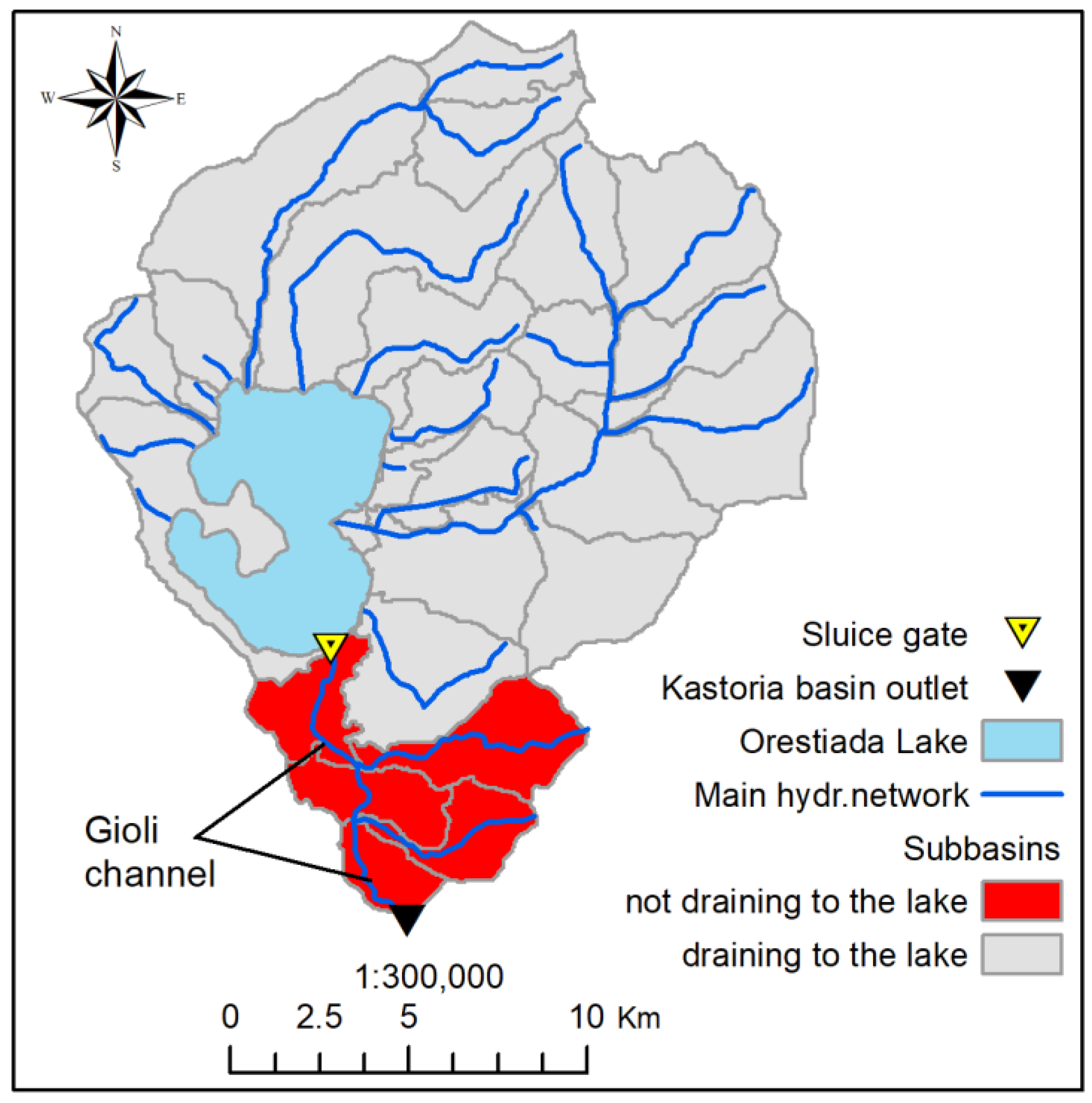
2.1. Study Site

The study area is the Orestiada Lake of the Kastoria hydrologic basin in northwestern Greece (40°30′45″N; 21°18′10″E) (Figure 1a). The maximum allowed lake surface elevation (LSE) is at 628.19 m above sea level (a.s.l.) with a maximum lake depth of ~9.1 m. Values above the maximum LSE can flood the residential areas around the lake, especially the city of Kastoria, which is at the eastern coast of the lake. For this reason, at the southern coast of the lake, water is discharged through a sluice gate to Gioli channel (Figure 1a). The bed and the upper edge of the sluice gate is at 624.95 and 627.45 m (a.s.l.), respectively. The end of Gioli channel is the final outlet of Kastoria basin and it is connected to Aliakmon river basin (Figure 1a) [25,26]. The local lake management authorities follow a program of water discharge in order to maintain a secure lake surface elevation at ~627 m (a.s.l.), which is accomplished by opening for a few days per month (~2 days per month on average) the sluice gate with a mean approximate rate of discharge ~2-3 m³/s. The water discharge from the lake satisfies also other purposes such as:

• improvement of lake water quality by using the inflow of cooler and denser water for flushing out the warmer lake water [27,28,29]. In this way, a reduction of primary production rates is accomplished, which is necessary because the lake is currently classified as eutrophic with a tendency to hypertrophication [27,30,31].
• partial water contribution to Aliakmon river (Figure 1a) for preserving its minimum ecological flow and for the production of hydropower by hydroelectric dams at its downstream sections.

The spatial variation of mean annual precipitation and temperature of Kastoria basin is given in Figure 1b,c, respectively [32]. The basin climate is classified as Cfb for the lowlands and Dfb for the uplands at the northern area according to the revised Köppen Geiger classification system of Peel et al. [33]. The coverage of land uses in the study area according to Corine Land Cover 2012 [34] database is approximately 36.4% agricultural lands (AGRI), 17.5% forests (FOR), 9.7% water bodies (WAT), 34.1% scrub and/or herbaceous vegetation associations (SHVEG) and 2.3% artificial surfaces and urban fabric (ARTS) (Figure 1d). The coverage of soil texture classes in the study area consists of Loamy Sand (3.9%), Sandy Loam (47.3%), (Loam 9.6%), Sandy Clay Loam (4.7%), (Clay 34.9%) according to the ESDB-ESDAC soil database [35,36] with sand increasing with altitude and the clayey soils dominating to the lowlands areas around the lake.

2.2. Data

The data used for the implementation of this study are the daily minimum, maximum, mean temperature and precipitation data from the Kastoria meteorological station (632 m, 40°30′38″N; 21°15′15″E) for the period 1/5/2012–31/4/2018 (Figure 2a,b) and the variation of lake surface elevation (LSE) (Figure 2c). This period corresponds to 6 full years with starting date the 1st of May for each year. For the specific period, the mean annual superficial discharge Q_d of the lake to Gioli channel through the sluice gate was estimated at 5.6 million m³/year (based on records of the Environmental and Spatial Planning Agency of Western Macedonia Prefecture, Department of Environment and Hydroeconomy).

Additional GIS datasets and databases used for this study include:

• The digital elevation model of the Kastoria basin obtained by the EU-DEM v1.1 database [37] with a spatial resolution of 25 m (Figure 1a).
• The bathymetry map of Orestiada lake designed for reference LSE = 628.00 m a.s.l. with isolines of 0.5 m depth [38] (Figure 1e).
• The average monthly climate data for minimum, mean, maximum temperature and precipitation of the recent past (1970-2000, WorlClim Version 2 database) and the respective parameters based on 19 general circulation models (GCMs) for three scenarios (RCP2.6, RCP4.5 and RCP8.5 according to IPCC/CMIP5) of future climate conditions (mean conditions of 2061-2080 period) derived from the WorldClim Version 1 database [39] (

  Table 1. Climatic data in raster format of 30 arc-sec (~1 km²) based on 19 GCMs for the three climate change scenarios (RCP2.6, RCP4.5 and RCP8.5) according to IPCC5/CMIP5 (WorldClim database [39]).

  No.	GCM	Code	RCP2.6 (n = 15)	RCP4.5 (n = 19)	RCP8.5 (n = 17)
  1	ACCESS1-0	AC	NA1	√	√
  2	BCC-CSM1-1	BC	√	√	√
  3	CCSM4	CC	√	√	√
  4	CESM1-CAM5-1-FV2	CE	NA	√	NA
  5	CNRM-CM5	CN	√	√	√
  6	GFDL-CM3	GF	√	√	√
  7	GFDL-ESM2G	GD	√	√	NA
  8	GISS-E2-R	GS	√	√	√
  9	HadGEM2-AO	HD	√	√	√
  10	HadGEM2-CC	HG	NA	√	√
  11	HadGEM2-ES	HE	√	√	√
  12	INMCM4	IN	NA	√	√
  13	IPSL-CM5A-LR	IP	√	√	√
  14	MIROC-ESM-CHEM	MI	√	√	√
  15	MIROC-ESM	MR	√	√	√
  16	MIROC5	MC	√	√	√
  17	MPI-ESM-LR	MP	√	√	√
  18	MRI-CGCM3	MG	√	√	√
  19	NorESM1-M	NO	√	√	√

  ¹ NA: not available in WorldClim database.

  ). The datasets are in raster form with spatial resolution of 30 arc-sec (~1 km²). The WorldClim database also provides the results of RCP6.0 scenario from the respective GCMs, but it was not used because it showed very small differences with the RCP4.5 for the study area.
• The local revised coefficients of Hargreaves and Samani equation [40] provided by Aschonitis et al. [41] were also used for achieving equivalent estimations of reference crop evapotranspiration, ET_o, with the complete formula of ASCE/FAO-56 method for short grass [42,43]. The revised coefficients have been produced based on the WorldClim database and they are provided in raster format with 30 arc-sec (~1 km²) spatial resolution [41].

2.3. Method for Analyzing the Hydroclimatic Vulnerability of a Lake/Reservoir

2.3.1. Case 1: No Outflows Outside the Drainage Basin of the Lake, Original Method of Bracht-Flyr et al.

The hydroclimatic model of Bracht-Flyr et al. [21] considers a simplified water balance for lakes assuming steady-state conditions. According to this model, the general mean annual water balance of a lake for a multiyear period is described by:

$$\mathsf{\Delta }{V}_{\mathrm{L}}=A_{\mathrm{L}}\left(P_{\mathrm{L}}-E_{\mathrm{L}}\right)+R_{\mathrm{B}}{A}_{\mathrm{B}}+G_{\mathrm{in}}-G_{\mathrm{out}}$$

(1)

where ΔV_L is the net annual change in the lake volume (L³), A_L is the lake surface area (L²), P_L is the mean annual precipitation over the lake (L), E_L is the mean annual evaporation from the lake (L), R_B is the mean annual runoff/recharge generated by the terrestrial area of the basin that drains to the lake (L), A_B is the contributing basin area that drains to the lake (L²), and G_in, G_out are the mean annual incoming and outgoing groundwater fluxes to and from the lake (L³), respectively. Assuming that an equilibrium condition is attained between all the inflows and outflows from the lake volume (ΔV_L≈0) and that a net groundwater transfer is negligible (G_in≈G_out), Equation (1) is simplified according to the following:

$$A_{\mathrm{L}}\left(P_{\mathrm{L}}-E_{\mathrm{L}}\right)+R_{\mathrm{B}}{A}_{\mathrm{B}}=0$$

(2a)

$$A^{\prime }=\frac{A_{\mathrm{B}}}{A_{\mathrm{L}}}=\frac{E_{\mathrm{L}}-P_{\mathrm{L}}}{R_{\mathrm{B}}}$$

(2b)

where A′ is the ratio of basin surface that drains to the lake versus the lake surface. The R_B parameter is described by the following equation [21,44]:

$$R_{\mathrm{B}}=P_{\mathrm{B}}\left[1-f_1\left(\mathsf{\Phi },{\mathsf{\omega }}_1\right)\right]$$

(3a)

where

$$\mathsf{\Phi }=\frac{E_{\mathrm{p}\mathrm{B}}}{P_{\mathrm{B}}}$$

(3b)

$$f_1\left(\mathsf{\Phi },{\mathsf{\omega }}_1\right)=\frac{1+{\mathsf{\omega }}_1\mathsf{\Phi }}{1+{\mathsf{\omega }}_1\mathsf{\Phi }+{\mathsf{\Phi }}^{-1}}$$

(3c)

where E_pB and P_B are the mean annual potential evapotranspiration and precipitation (L) of the basin surface that drains to the lake and ω₁ is an empirical factor that represents the effects of soil and land use that both regulate real evapotranspiration. f₁(Φ,ω₁) is an asymptotic function that ranges between 0-1.

Bracht-Flyr et al. [21] made the assumption of uniform climate conditions in the whole basin of the lake and provided the following simplified form:

$$\frac{A_{\mathrm{B}}}{A_{\mathrm{L}}}=\frac{E_{\mathrm{p}}-P}{P\left[1-f_1\left(\mathsf{\Phi },{\mathsf{\omega }}_1\right)\right]}={A_1}^{\prime }$$

(4a)

where

$$\mathsf{\Phi }=\frac{E_{\mathrm{p}}}{P}$$

(4b)

where E_p and P are the mean annual potential evapotranspiration and precipitation (L) of the whole basin (including the lake), respectively. Equation (4) works only for water-limited conditions (Φ≥1) and not for energy limited ones (Φ < 1). In the second case, the formation of a lake under a stationary climate would be permanent and solely controlled by topography for maintaining constant dimensions [21]. For steady-state conditions, it is easy to estimate the ω₁ parameter using available climatic data of the basin and using the current A_B/A_L ratio.

The function f₁ (Equation (3c)) is a Budyko-type function [23,24] and describes the term ET_a/P, where ET_a is the mean annual actual evapotranspiration [21,44,45], which is given by the following equation:

$$E{T}_{\mathrm{a}}=P\cdot f_1\left(\mathsf{\Phi },{\mathsf{\omega }}_1\right)$$

(5)

The ω₁ value can vary depending on the soil type, land use and the method used for estimating potential evapotranspiration [44,45,46]. Zhang et al. [46] noted that ω₁ is a lumped factor that represents the integrated effect of multiple basin processes and land cover conditions on evapotranspiration.

Assuming that the basin features (e.g., land uses, soil properties, etc.) that regulate ω₁ value remain constant (i.e., ω₁ remains constant in the future), then the changes in the term A′ using climatic data derived from GCMs for different future climate projections can be assessed.

The approach of Bracht-Flyr et al. [21] is interesting and constitutes a useful tool for types of analysis as the aforementioned one, but there are some aspects in the methodology that need to be clarified. For example, the initial assumption that was made for model building was that the system is closed (Equation (1)) while for building the final empirical model of Equations (4) and (5), other additional assumptions were made (e.g., uniform evapotranspiration in the whole A_T, Budyko-type of real evapotranspiration described by Equation (5). If we consider that there are no other factors that extract water from the A_T basin and that the initial assumption of closed system is still valid, then the final water balance under steady-state conditions for the A_T area should simply be described as P-ET_a = 0. In this case, and under a water limited environment (Φ>1), the Budyko-type function of ET_a (Equation (5)) requires a value of ω₁→+∞ for achieving P-ET_a≈0. Thus, in a theoretical steady-state and water-limited environment (Φ>1) of a closed lake basin with 100% natural landscape and water losses only by evapotranspiration, it is expected ω₁→+∞. The above indicate that a lake basin system where the ET_a is described by Equation (5) with a regular ω₁ value (e.g., <10) [45,46], cannot support the initial assumption of a closed system because P-ET_a will be always >0, which consequently means that there are additional water extraction factors for preserving the system under steady state conditions.

Based on the above, if we consider that the initial assumption of “closed system” is violated because (a) it is more probable other factors of water extraction exist and (b) the Budyko-type of real evapotranspiration is valid based on a regular ω₁ value (i.e., not reaching +∞), then the final water balance under steady conditions in the A_T basin should be described by:

$$P-E{T}_{\mathrm{a}}-Q_{\mathrm{m}}=0$$

(6a)

$$Q_{\mathrm{m}}=P-E{T}_{\mathrm{a}}$$

(6b)

where Q_m is the annual amount of water extraction (L) from the system of A_T basin by factors not related to ET_a (e.g., groundwater recharge outside the A_T, net industrial/domestic water consumption inside the A_T without return flows etc). Violating the initial assumption of closed system affects also the ω₁ value because the larger Q_m is, the smaller ω₁ will be.

2.3.2. Case 2: Outflows Outside the Drainage Basin of the Lake (Modified Method)

In many LRs, as in the case of Orestiada Lake, steady-state conditions may be preserved because water is superficially discharged outside the A_T area (e.g., typical case of a reservoir with hydroelectric dam, where water is discharged for energy production or a reservoir used for irrigating downstream areas). In such cases, Equation (4) can be modified as follows using an additional factor f₂ according to the following:

$$\frac{A_{\mathrm{B}}}{A_{\mathrm{L}}}=\frac{E_{\mathrm{p}}-P}{P\left[1-f_1\left(\mathsf{\Phi },{\mathsf{\omega }}_1\right)-f_2\left(\mathsf{\Phi },{\mathsf{\omega }}_2\right)\right]}=A^{\prime }$$

(7)

where

$$Q_{\mathrm{d}}=P\cdot f_2\left(\mathsf{\Phi },{\mathsf{\omega }}_2\right)$$

(8a)

$$f_2\left(\mathsf{\Phi },{\mathsf{\omega }}_2\right)=1-\frac{1+{\mathsf{\omega }}_2\mathsf{\Phi }}{1+{\mathsf{\omega }}_2\mathsf{\Phi }+{\mathsf{\Phi }}^{-1}}$$

(8b)

where Q_d is the mean annual amount of water (L) that superficially discharges outside the A_T area for maintaining steady state conditions of the LR, and ω₂ is the coefficient that regulates the rate of superficial discharge. The f₂(Φ,ω₂) is also an asymptotic function that ranges between 0-1 but with inverted shape compared to f₁(Φ,ω₁), which denotes that the higher is the ET_a and Φ, the lower will be the Q_d. If the mean annual values of Q_d, E_p, P and A′ are known for a relatively large period of years then Equation (8a) can be used for estimating ω₂ and Equation (7) for estimating ω₁ using ω₂. We have to note that any abstraction or water outflow from the lake that returns to A_T (e.g., using lake water for irrigation inside A_T) is not considered in the Q_d.

Moreover, an additional modification was made by substituting the term of mean annual potential evapotranspiration E_p with the term of mean annual reference evapotranspiration ET_o in Φ calculation (i.e., Φ = ET_o/P) of Equations (7) and (8). The ET_o is calculated by the formula of Hargreaves and Samani [40]:

$$E{T}_{\mathrm{o},\mathrm{d}}=c_{\mathrm{hs}2}\cdot \left(T_{\mathrm{mean}}+17.8\right)\cdot \frac{R_{\mathrm{a}}}{\mathsf{\lambda }}\cdot {\left(TD\right)}^{0.5}$$

(9)

where ΕΤ_ο,d is the reference evapotranspiration (mm d⁻¹), R_a is the daily extraterrestrial radiation (MJ m⁻²), λ is the latent heat of vaporization (2.45 MJ kg⁻¹), T_mean is the mean daily temperature estimated as the average value of maximum and minimum daily temperature (°C), TD is the difference between maximum and minimum daily temperature (°C) and c_hs2 is a recalibrated coefficient that corrects the original Hargreaves-Samani equation in order to be equivalent to ASCE/FAO-56 method for short reference crop [42,43]. The original value of c_hs2 is 0.0023, while the local recalibrated c_hs2 values for any place of the world can be obtained by Aschonitis et al. [41].

Using the climate conditions of a relatively large period of years where the LR is under steady-state conditions due to superficial outflows outside the A_T (meaning that Q_d, ET_o, P and A′ are known parameters), then ω₂ is estimated after re-arranging the parameters of Equation (8a) as follows:

$$\frac{1+{\mathsf{\omega }}_2\mathsf{\Phi }}{1+{\mathsf{\omega }}_2\mathsf{\Phi }+{\mathsf{\Phi }}^{-1}}=1-\frac{Q_{\mathrm{d}}}{P}$$

(10a)

$${\mathsf{\omega }}_2=\frac{\mathsf{\Phi }-\mathsf{\Phi }\cdot X-X}{{\mathsf{\Phi }}^2\left(X-1\right)}$$

(10b)

where

$$X=1-\frac{Q_{\mathrm{d}}}{P}$$

(10c)

Using the estimated ω₂ from Equation (10b), ω₁ can also be estimated after re-arranging the parameters of Equation (7) as follows:

$$\frac{1+{\mathsf{\omega }}_1\mathsf{\Phi }}{1+{\mathsf{\omega }}_1\mathsf{\Phi }+{\mathsf{\Phi }}^{-1}}=\frac{1+{\mathsf{\omega }}_2\mathsf{\Phi }}{1+{\mathsf{\omega }}_2\mathsf{\Phi }+{\mathsf{\Phi }}^{-1}}-\frac{E{T}_o-P}{P\cdot A^{\prime }}$$

(11a)

$${\mathsf{\omega }}_1=\frac{\mathsf{\Phi }-\mathsf{\Phi }\cdot Y-Y}{{\mathsf{\Phi }}^2\left(Y-1\right)}$$

(11b)

where

$$Y=\frac{1+{\mathsf{\omega }}_2\mathsf{\Phi }}{1+{\mathsf{\omega }}_2\mathsf{\Phi }+{\mathsf{\Phi }}^{-1}}-\frac{E{T}_o-P}{P\cdot A^{\prime }}$$

(11c)

where Equations (10) and (11) are valid for Φ = ΕΤ_ο/P>1, P≠0, X≠1 and Y≠1. The rule Y≠1 denotes that Q_d is always ≠0. For Q_d = 0 the original Bracht-Flyr et al. [21] method should be used.

Using the same assumptions of Section 2.3.1. for deriving Equation (6), the final water balance under steady conditions in the A_T basin for Q_d≠0 is described by:

$$P-E{T}_{\mathrm{a}}-Q_{\mathrm{d}}-Q_{\mathrm{m}}=0$$

(12a)

$$Q_{\mathrm{m}}=P-E{T}_{\mathrm{a}}-Q_{\mathrm{d}}$$

(12b)

where Q_m is the annual amount of water extraction (L) from the system of A_T basin by other factors not related to Q_d and ET_a (e.g., groundwater recharge outside the A_T, net industrial/domestic water consumption inside the A_T without return flows etc).

2.3.3. Estimating LR Conditions under the Effects of Climate Change

The modified method (Equations (7)–(12)) allows evaluating the LR conditions under climate change considering that a) any changes in future soil and land use management or other basin characteristics do not alter the ω₁ value and b) Q_d is always ≠ 0 and the Q_d rates are defined by the future P and Φ considering a stable shape of f₂ function (i.e., ω₂ remains constant). For example, in the case of Orestiada Lake, it is assumed that outflow continues to exist with Q_d rates regulated by Equstion 8a despite the fact that LSE may fall below the bed elevation of the sluice gate. Under such conditions, the final A_B/A_L ratio is equal to A′ (Equation (7)) considering that lake water is pumped and guided to Gioli channel in order to preserve the outflow for improving lake water quality, the minimum ecological flow and the hydropower production of Aliakmon river as described in the “Study site” section (pumping water from Orestiada Lake to Gioli channel could be a realistic case if we consider a similar effect of climate change on the whole Aliakmon river basin). The aforementioned strategy is denoted as “strategy S1” and the results of A′ lake volume V_L, superficial outflow Q_d, real evapotranspiration ET_a and other extractions Q_m of the final steady state conditions are symbolized as A_S1′, V_L,_S1, Q_d,S1, ET_a,S1, and Q_m,S1, respectively.

Taking into account the results of the aforementioned procedure, any deviation from the current climate conditions could indicate what the final expected steady-state conditions (A_S1′, V_L,_S1, Q_d,S1, ET_a,S1, and Q_m,S1) will be even before they occur. This allows designing alternative strategies for the volume preservation of LR based on the estimated Q_d,S1 under climate change. For example, the estimated Q_d,S1 can be returned to LR (in reality Q_d,S1 is just calculated but it is not discharged) for restoring LR’s volume at any time, even before V_L,S1 reaches its final steady-state condition. If we set a minimum threshold value of lake volume (V_L,th) for which S1 strategy should stop and the estimated Q_d,S1 should return to/remain in LR (denoted as Strategy S2) then we can estimate a respective minimum time in years that is required for restoring LR volume to the initial conditions as follows:

$$t_{\mathrm{S}2}=\frac{V_{\mathrm{L},0}-V_{\mathrm{L},\mathrm{th}}}{Q_{\mathrm{d},\mathrm{S}1}}\mathrm{for}{V}_{\mathrm{L},0}>V_{\mathrm{L},\mathrm{S}1}$$

(13a)

$$t_{\mathrm{S}2}=0\mathrm{for}{V}_{\mathrm{L},0}\le V_{\mathrm{L},\mathrm{S}1}$$

(13b)

where t_S2 is the minimum time (years) that it is required for restoring LR volume to V_L,0 from V_L,th condition, V_L,0 is the LR volume at the initial/current conditions (L³), V_L,th is the minimum threshold value of lake volume (L³) for which S1 strategy should stop and Q_d,S1 should return to/remain in the lake. Q_d,S1 is expressed in volume units (L³) in Equation (13a). The term “minimum time” for t_S2 is used because at the initiation of S2 strategy, the lake volume is not at steady state conditions and still declines until reaching V_L,S1 (case of Equation (13a)). Thus, the annual Q_d,S1 are added to an initial volume which continues declining. Thus, the real time for LR volume recovery is expected to be longer. In this study, as V_L,th was set the lake volume that corresponds to LSE at the bed of the sluice gate while V_L,0 corresponds to the mean volume of Orestiada Lake during the period 1/5/2012-31/4/2018 (i.e., current conditions).

2.4. Linking A′ Parameter to Lake Water Volume

The lake area, A_L, and the lake water volume, V_L, can be estimated for different lake surface elevations when the bathymetry of LR is known. A_B and A′ parameter (A_B/A_L ratio) can also be estimated for each LSE value when the total area A_T (A_T = A_B+A_L) of the basin is known. Thus, each value of LSE can be linked to specific values of A_L, A_B, A′ and V_L.

In this study, the isolines of bathymetry of Orestiada Lake were used to develop a triangulated irregular network (TIN) of the lake bed. The TIN was used to determine the lake surface A_L and volume V_L for different values of LSE using the tool {SurfaceVolume} from 3D Analyst toolbox of Arc-GIS 10.1 (ESRI). The Arc-Hydro module of ArcSWAT model [47] was also used to delineate the total area of Kastoria basin that drains to Orestiada lake including the lake (i.e., A_T). The known value of A_T and the values of A_L for different LSEs were used to calculate the respective A_B and A′ values. In this way, the A′ values were linked to V_L for different LSEs.

2.5. Using Meteorological Stations as Descriptors of the Whole Basin Climate

There are various methods (e.g., Thiessen polygons, interpolation methods, temperature, rainfall gradients, etc.) for deriving the mean annual P and ET_o for basins that have a good number and distribution of meteorological stations. On the other hand, there are basins that may not have an adequate number of stations and especially basins with large portions of non-accessible mountainous areas where meteorological stations usually do not exist. In such cases, the derivation of the mean annual P and ET_o of the basin from a few stations may not be representative for the whole basin. One solution to this problem is to use gridded climatic data that have been produced by GCMs and advanced interpolation methods that take into account topographic characteristics for achieving finer grid resolutions (e.g., such gridded data are those provided by WorldClim database, e.g., Figure 1b,c). The average pixels’ value of the WorldClim gridded mean monthly data of precipitation, maximum and minimum temperature of recent past (1970-2000) and future climate scenarios (Table 1) were extracted from the polygon that corresponds to A_T. The respective values were also extracted from the specific pixel that corresponds to the meteorological station of Kastoria (Figure 1a). Thus, twelve mean monthly values of precipitation, maximum and minimum temperature from the grids of the 51 simulation scenarios of GCMs (Table 1) plus the case of the (1970-2000) (52 cases × 12 months for each parameter) were extracted for the position of the station and for the whole A_T basin. These values were used through regression analysis to develop three linear functions (g₁, g₂, g₃) that calculate the mean monthly values of T_max,T, T_min,T and P_T of the drainage basin (defined by A_T) using the respective parameters from the position of Kastoria station, respectively:

$$T_{\max ,\mathrm{T}}=g_1\left(T_{\max ,\mathrm{S}}\right),T_{\min ,\mathrm{T}}=g_2\left(T_{\min ,\mathrm{S}}\right),P_{\mathrm{T}}=g_3\left(P_{\mathrm{S}}\right)$$

(14)

where P_S, T_max,S, T_min,S are the mean monthly precipitation, maximum and minimum temperature at the position of the Kastoria meteorological station, and P_T, T_max,T, T_min,T are the mean monthly precipitation, maximum and minimum temperature of the A_T basin.

The calibrated Equation (14a)–(14c) were finally used to convert the observed data of monthly P_S, T_max,S, T_min,S of the station for the period 1/5/2012–31/4/2018 to the respective mean values of the A_T basin. These values were further used to calculate ET_o with Equation (9) and Φ of A_T for the respective period. We have to note that mean temperatures are calculated as the average of minimum and maximum temperature in all cases.

3. Results

3.1. Bathymetry, Lake Volume, and A′ Parameter for Different Lake Surface Elevations (LSEs)

The TIN surface of Orestiada lake bed was created taking into account the 0.5 m isolines of bathymetry (Figure 1e). The TIN was used to determine the lake surface A_L and volume V_L for different values of LSE (

Table 2. Lake surface A_L, lake volume V_L, basin area that drains to the lake A_B, A_B/A_L and mean depth of the lake for different values of lake surface elevation (LSE) considering A_T = 272.48 km² (grey zone plus the lake in Figure 3).

LSE (m a.s.l.)	Fall from Reference Elevation (m)	AL (km2)	VL (m3 × 106)	AB (km2)	A′	Mean Depth (m)
628.0	0	30.777	113.413	241.706	7.8535	3.68
627.5	−0.5	28.455	98.653	244.027	8.5759	3.47
627.0	−1	27.175	84.748	245.307	9.0269	3.12
626.5	−1.5	26.079	71.436	246.404	9.4484	2.74
626.0	−2	25.024	58.661	247.458	9.8888	2.34
625.5	−2.5	23.867	46.439	248.615	10.417	1.95
625.0	−3	22.305	34.898	250.178	11.216	1.56
624.5	−3.5	19.755	24.365	252.727	12.793	1.23
624.0	−4	15.677	15.464	256.806	16.381	0.99
623.5	−4.5	11.493	8.600	260.990	22.709	0.75
623.0	−5	5.968	4.060	266.515	44.657	0.68
622.5	−5.5	2.834	1.889	269.649	95.158	0.67
622.0	−6	1.300	0.848	271.182	208.58	0.65
621.5	−6.5	0.514	0.352	271.969	529.61	0.69
621.0	−7	0.269	0.163	272.214	1012.6	0.61
620.5	−7.5	0.133	0.060	272.349	2043.1	0.45
620.0	−8	0.046	0.013	272.436	5866.7	0.29
619.5	−8.5	0.006	0.001	272.476	43072.4	0.20

).

The Arc-Hydro module delineated the total area of Kastoria basin (308.6 km²) and created 26 subbasins from which 21 drain to the lake while 5 drain directly to Gioli channel at the southern part of the lake towards the outlet of the Kastoria basin (Figure 3). The total area A_T of the 21 subbasins that drain to the lake (including the area of the lake) was estimated A_T = 272.48 km². Thus, using the value of A_T, the values of A_B and A′ were estimated based on the respective values of A_L for different LSEs (Table 2).

3.2. Estimating ω₁ and ω₂ for the Current Period (1/5/2012–31/4/2018)

The WorldClim gridded mean monthly data of precipitation, maximum and minimum temperature of recent past (1970–2000) and future climate scenarios (Table 1) were extracted (a) from the total basin of A_T = 272.48 km² (mean value of pixels in the basin) and (b) from the specific pixel that corresponds to the meteorological station of Kastoria (Figure 1a). Thus, 52 × 12 pairs of (T_max,T, T_max,S), (T_min,T, T_min,S) and (P_T, P_S) were developed in order to calibrate the functions g₁, g₂ and g₃ (Equations (14a)–(14c)) through linear regression. The g₁, g₂ and g₃ functions were the following T_max,T = 0.99T_max,S-1.128 with R² = 0.99, T_min,T = 0.988T_min,S -1.063 with R² = 0.99 and P_T = 0.928P_S + 3.515 with R² = 0.99.

The monthly T_max,T, T_min,T and P_T of the A_T basin for the study period 1/5/2012–31/4/2018 were estimated based on the calibrated g₁, g₂ and g₃ functions and using the respective monthly observed data of T_max,S, T_min,S and P_S of Kastoria station. The monthly T_max,T and T_min,T of the A_T basin were also used to estimate the monthly Hargreaves-Samani ET_o values (Equation (9)) of the basin using c_hs2 = 0.002087 (average c_hs2 value of pixels included in A_T) from the database of Aschonitis et al. [41]. Finally, the mean annual P and ET_o of the A_T for the 2012-2018 period were estimated at 701 and 968 mm per year, respectively. The mean observed superficial discharge to Gioli channel of the respective period was 5.6 million m³/year, which corresponds to Q_d = 20.6 mm per year. The mean LSE of the study period was 626.99 m, which corresponds to A′ = 9.06 and V_L = 84.61 million m³ (estimated based on linear regressions between sequential values of Table 2). Using the mean annual values of P = 701 mm, ET_o = 968 mm, Φ = ET_o/P = 1.381, Q_d = 20.6 mm and A′ = 9.06, the ω₂ value was found equal to 16.56 according to Equation (10c). Using this ω₂ value, the ω₁ value was found equal to 6.09 according to Equation (11c). Using Equation (5), the mean annual real evapotranspiration ET_a of the studied period was found equal to 651 mm while Q_m was estimated equal to 29.4 mm per year according to Equation (12b) (equivalent to 8.1 million m³ per year).

The responses of f₁ (Equation (3c)) and f₂ (Equation (8b)) functions versus Φ using the ω₁ = 6.09 and ω₂ = 16.56 are given in Figure 4. For comparative purposes, Figure 4 also includes the response of f₁ using ω₁ = 0.1 for basins with sandy soils and sparse vegetation (case of basin from Nebraska Sand Hills, USA [45]), ω₁ = 2.55 for grass-covered basins (75% grass-covered), ω₁ = 2.84 for forest-covered basins (75% tree-covered) (both values are from Australian basins of the east coast [46]) and ω₁ = 5.0 (a case that was observed in [45,46]).

3.3. Estimating A′ and Respective Lake Volumes based on Climate Change Scenarios and Water Management Strategies

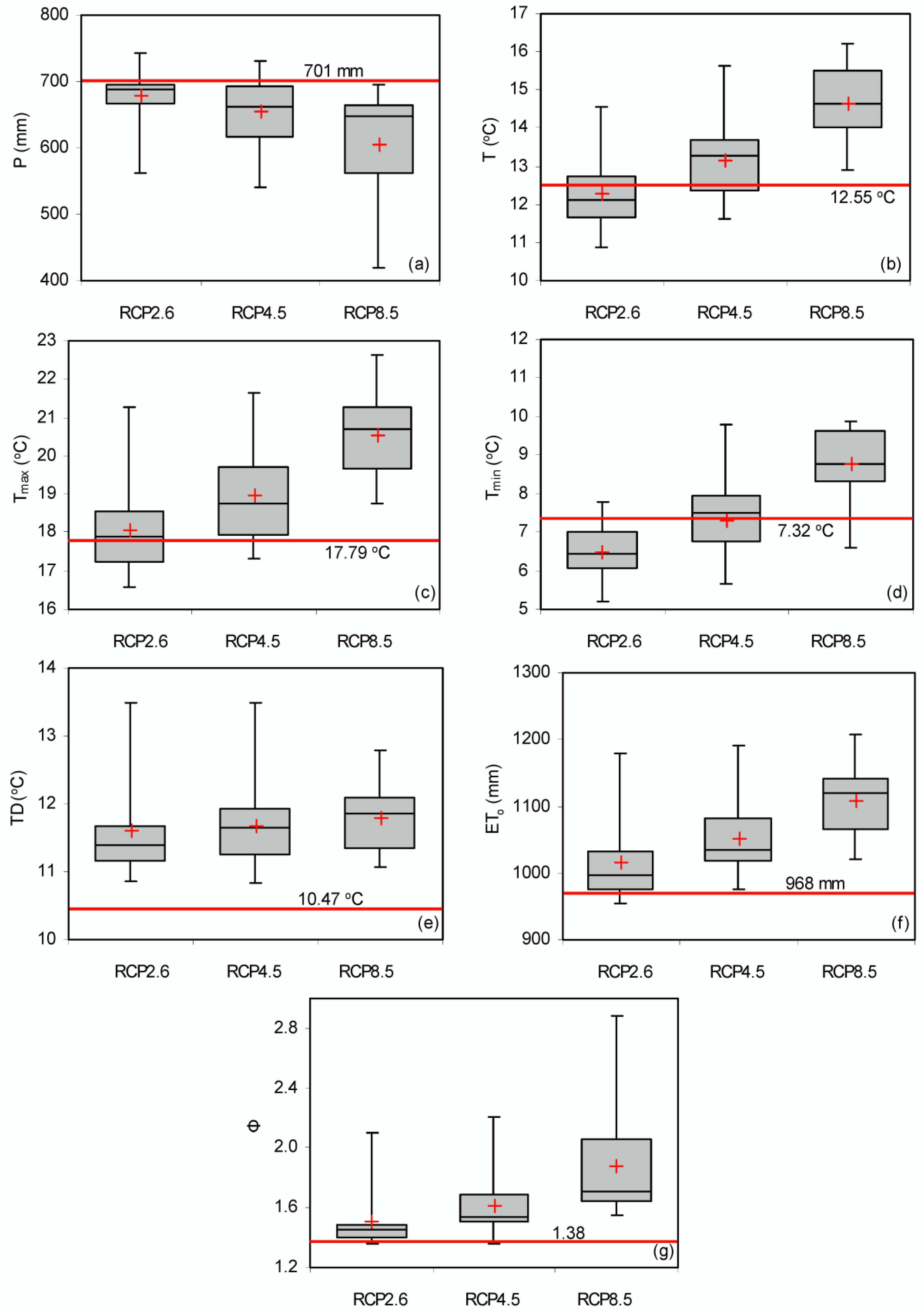
3.3.1. Trends of Climate in the A_T of Orestiada Lake according to GCMs for Different Climate Change Scenarios

The box-whisker plots of mean annual values of P, T, T_max, T_min, TD, ET_o and Φ = ET_o/P of GCMs for each climate change scenario (RCP2.6, RCP4.5, RCP8.5) are given in Figure 5a–g, respectively. For comparison purposes, the current mean annual values of the aforementioned parameters for the period 1/5/2012–31/4/2018 are also given as red lines in Figure 5a–g. The mean trends of P, T, T_max, T_min, TD, ET_o and Φ of GCMs for each climate change scenario (red crosses in Figure 5a–g) were compared with the mean annual conditions of the period 1/5/2012–31/4/2018 (red lines) in order to evaluate the percent changes from current conditions (

Table 3. Maximum negative, average, standard deviation and maximum positive % of changes in mean annual values of P, T, T_max, T_min, TD, ET_o, Φ, V_L,S1, Q_d,S1, ET_a,S1 and Q_m,S1 estimated based on the GCMs for RCP2.6, RCP4.5, RCP8.5 in comparison to the respective mean annual values of the period 1/5/2012-31/4/2018.

Parameter	% Change	RCP2.6	RCP4.5	RCP8.5	Parameter	% Change	RCP2.6	RCP4.5	RCP8.5
P	Max.neg.	−19.8%	−22.8%	−40.3%	Φ	Max.neg.	−1.8%	−1.8%	12.0%
	Average	−3.1%	−6.5%	−13.7%		Average	9.2%	17.2%	36.0%
	St.dev.	5.9%	7.6%	11.9%		St.dev.	13.5%	14.2%	26.1%
	Max.pos.	6.1%	4.1%	−0.9%		Max.pos.	51.8%	59.7%	109.2%
T	Max.neg.	−13.2%	−7.3%	2.7%	VL,S1	Max.neg.	−95.7%	−96.2%	−98.6%
	Average	−2.2%	4.7%	16.7%		Average	−52.8%	−75.6%	−90.3%
	St.dev.	7.6%	8.7%	8.4%		St.dev.	33.6%	26.2%	5.6%
	Max.pos.	15.8%	24.5%	29.3%		Max.pos.	26.1%	25.3%	−79.8%
Tmax	Max.neg.	−6.8%	−2.7%	5.5%	Qd,S1	Max.neg.	−63.9%	−68.5%	−85.7%
	Average	1.6%	6.6%	15.5%		Average	−14.4%	−27.3%	−46.3%
	St.dev.	7.1%	7.1%	6.8%		St.dev.	18.2%	18.7%	20.2%
	Max.pos.	19.6%	21.7%	27.2%		Max.pos.	10.5%	8.3%	−23.8%
Tmin	Max.neg.	−29.1%	−22.7%	−9.9%	ETa,S1	Max.neg.	−16.5%	−19.4%	−36.9%
	Average	−11.5%	−0.2%	19.5%		Average	−2.3%	−4.9%	−11.3%
	St.dev.	9.5%	13.3%	13.2%		St.dev.	5.0%	6.9%	11.3%
	Max.pos.	6.5%	33.5%	35.0%		Max.pos.	5.9%	4.6%	1.1%
TD	Max.neg.	3.8%	3.4%	5.7%	Qm,S1	Max.neg.	−61.10%	−65.88%	−83.99%
	Average	10.8%	11.4%	12.7%		Average	−13.53%	−25.53%	−43.90%
	St.dev.	6.5%	5.8%	5.0%		St.dev.	17.23%	17.90%	20.17%
	Max.pos.	28.8%	28.8%	22.3%		Max.pos.	9.73%	7.54%	−22.05%
ETo	Max.neg.	−1.5%	0.7%	5.3%
	Average	5.0%	8.7%	14.5%
	St.dev.	6.2%	5.8%	5.6%
	Max.pos.	21.7%	23.2%	24.8%

). The individual values for each GCM and climatic scenario that were used for creating the box-whisker plots of Figure 5a–g are given in the Supplementary Materials (Table S1).

The worst-case scenario of climate change was the one provided by the GFDL-CM3 (no.6 code GF in Table 1) for RCP8.5 where P showed a decrease of 283 mm (-40.3%), T showed an increase of 3.68 °C (+29.3%), T_max showed an increase of 4.84 °C (+27.2%), T_min showed an increase of 2.51 °C (+34.3%), TD showed an increase of 2.33 °C (+22.3%), ET_o showed an increase of 240 mm (+24.8%), while Φ was more than double, showing an increase of 109.2%, in comparison to the mean annual conditions of 1/5/2012–31/4/2018.

3.3.2. Effects of S1 and S2 Strategy on Orestiada Lake Conditions under Different Climate Change Scenarios

The final mean annual A_S1′ and Q_d,S1 of Orestiada lake and the ET_a,S1 and Q_m,S1 of A_T basin under the effects of S1 strategy and climate change were estimated by Equations (5), (7), (8a) and (12b), respectively, taking into account ω₁ = 6.09 and ω₂ = 16.56, and the future conditions defined by the GCMs of each future climate change scenario (Figure 5a–g, Table S1). The Q_d,S1 (mm) and Q_m,S1 (mm) values were converted to (m³ × 10⁶ per year) considering A_T = 272.48 km². The final A_S1′values were also expressed as lake volumes V_L,S1 (m³ × 10⁶) using Table 2 (through linear regression between 0.5 m intervals). The box-whisker plots of A_S1′, V_L,S1, Q_d,S1, ET_a,S1 and Q_m,S1 estimations according to S1 strategy for the climate projections of GCMs based on the three RCP scenarios are given in Figure 6a–e, respectively. For comparison purposes, the current mean annual values of the aforementioned parameters for the period 1/5/2012–31/4/2018 are also given as red lines in Figure 6a–e. The mean trends of V_L,S1, Q_d,S1, ET_a,S1 and Q_m,S1 of GCMs for each climate change scenario (red crosses in Figure 6b–e) were compared with the mean annual conditions of the period 1/5/2012–31/4/2018 (red lines) in order to evaluate the % changes from current conditions (Table 3). The individual values for each GCM and climatic scenario that were used for creating the box-whisker plots of Figure 6a–e are given in the Supplementary Materials (Table S2).

As regards the S2 strategy, the minimum time t_S2 for restoring the volume of LR was estimated taking into account that the mean annual lake volume for the current conditions of the period 1/5/2012-31/4/2018 is V_L,0 = 84.61 m³ × 10⁶ and that the lake volume that corresponds to the bed elevation of the sluice gate (LSE = 624.95 m a.s.l.) is V_L,th = 33.2 m³ × 10⁶. The box-whisker plots of t_S2 values for each RCP scenario are given in Figure 6f and Table S2.

Some interesting observations from the analysis of S1 and S2 strategies are the following:

• there were 2 GCM cases (no.9 HD for RCP2.6 and no.5 CN for RCP4.5) out of the 51 (all cases of the three scenarios) where the final V_L,S1 was greater than mean annual value V_L,0 of the period 1/5/2012-31/4/2018 (i.e., wetter future climatic conditions compared to the current ones). Thus, for these two cases, the t_S2 is 0 according to Equation (13b) for S2 strategy.
• 53.3% of GCM cases for RCP2.6, 94.7% of GCM cases for RCP4.5 and 100% of GCM cases for RCP8.5 showed V_L,S1<V_L,th (i.e., final lake volumes smaller than the volume that corresponds to the bed elevation of the sluice gate).

4. Discussion

4.1. Violation of the Assumption for Negligible Net Groundwater Transfer or Other Types of Outflows

Both the original (Equation (4)) and the modified method (Equation (7)) are based on the simplistic formula of Equation (2), which was built considering a negligible net groundwater transfer (G_in≈G_out). In both cases, this assumption was finally violated in order to close the water budget using Equations (6) and (12), respectively, considering additional terms for describing outflows outside the lake basin. This element could be considered to be a problem in the theoretical background but in reality it is not because the concept behind the formation of both models is (a) first to derive a simplistic formula as a base (i.e., Equation (2)) for building the models and (b) to introduce the terms f₁ and f₂ that convert Equation (2) to two semi-empirical models (Equation (4) or Equation (7)), which in reality are non-linear functions where their coefficients are calibrated. Thus, the two final semi-empirical models (Equations (4) and (7)) indirectly include the groundwater or other types of inflows-outflows (if they exist) because they are calibrated with actual data that may include such effects.

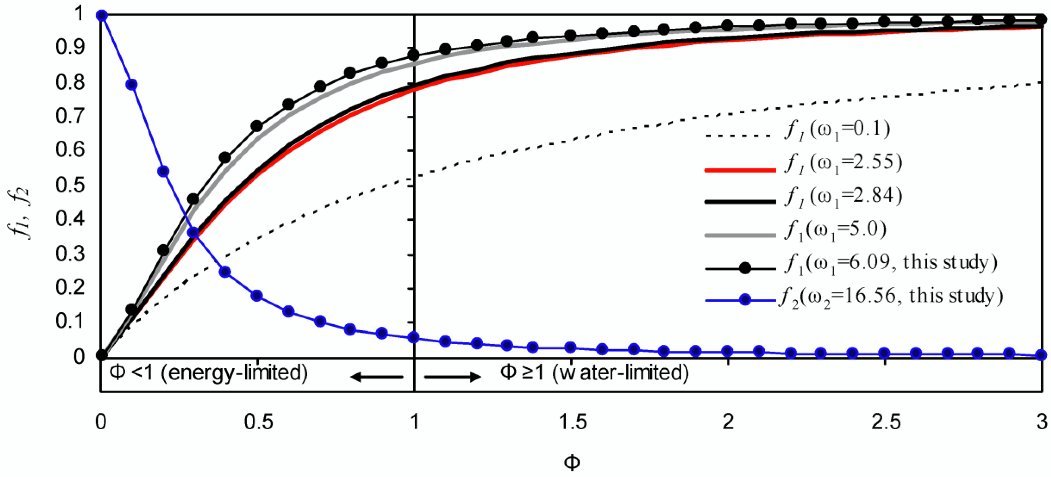
4.2. Validity of ω₁ in the Budyko Hypothesis and Justification of Q_m based on Local Factors

The validity of the final estimated steady-state water balance (Equations (6a) and (12a)) requires evaluation of the individual parameters (P, ET_a, Q_d, Q_m) based on expert judgement (especially the case of ET_a and Q_m parameters). The accuracy of mean P in A_T can be evaluated based on the availability, spatial distribution and accuracy of means that measure meteorological parameters, while Q_d purely depends on the authorities that manage the superficial outflows. On the other hand, ET_a and Q_m parameters are the parameters with the higher uncertainty and can be evaluated through indirect observations.

As regards ET_a, the estimated ω₁ = 6.09 based on the current conditions (1/5/2012–31/4/2018) may seem quite high but it is not unrealistic since similar values have been already observed in other studies [45,46]. Taking into account Figure 4, it is observed that for Φ = 1.38 (mean annual Φ of 1/5/2012–31/4/2018 for the study area), the f₁ for a sandy soil with sparse vegetation is f₁(ω₁ = 0.1) = 0.61, for a grass-covered basin is f₁(ω₁ = 2.55) = 0.86, for a forest-covered basin is f₁(ω₁ = 2.84) = 0.87 while for f₁(ω₁ = 6.09) = 0.928. These values indicate that for the same amount of P, the conditions of our study area would provide 34.3% higher ET_a from a respective basin covered with sandy soil and sparse vegetation, 7.3% higher ET_a from a respective mostly grass-covered basin, and 6.3% higher ET_a from a respective mainly forest-covered basin. These differences can be considered realistic and justifiable due to the following combined reasons:

• the lake covers ~10% of the A_T (Figure 3) where evaporation is non-limited and approximates ET_o [42]. Thus, the high percentage coverage of the lake in the A_T could be a basic factor that leads to a high value of ω₁.
• another reason of the high ω₁ value can also be the high percent (~30%) of agricultural land in the A_T area (Figure 1d). Summer irrigated crops and especially those in water limited environments (Φ>1) receive irrigation water for achieving maximum evapotranspiration rates during the summer period of low rainfall. In A_T area, the % of irrigated land is ~9.8% considering the agriculture statistics of Kastoria, Vitsi, Makethnon and Agioi Anargyroi municipalities [48], which are inside A_T. The rest winter non-irrigated crops (~20.2%) increase the water availability for their own evapotranspiration demands because they act as cover crops that can reduce runoff especially in areas of higher slopes [49,50]. Thus, the contribution of agricultural lands and especially of irrigated ones in the A_T, could also be a basic factor that leads to a higher value of ω₁.

Considering the above, the estimated ET_a rates by Equation (5) using ω₁ = 6.09 have a realistic base at least for the current conditions. As concern the future conditions, which predict smaller lake areas/volumes due to higher evapotranspiration and lower rainfall, we can assume that any possible reduction of ω₁ that could occur due the reduction of lake evaporative surface can be counterbalanced by the higher lake evaporation rates due to the shallower and warmer waters and by the higher evapotranspiration rates of irrigated agricultural lands due to the increase of temperature. The general reduction of ET_a of the whole A_T (Figure 5d) due to ET_o increase and P decrease can be justified by the fact that the available water for evapotranspiration will be reduced for the natural non-aquatic landscape and non-irrigated agricultural land that cover more than 80% of the A_T area.

The domestic water use and groundwater outflow are the two main factors that regulate the existence and rate of Q_m parameter. The local domestic water consumption is supplied from both ground and surface waters, while all the domestic wastewater goes to the wastewater treatment plant (WWTP) of Kastoria, which is near the Gioli channel. All the treated water is discharged to Gioli channel, thus the return flow to A_T by domestic water consumption is almost null. According to UNEP/MAP [51], the WWTP of Kastoria treated 5640 m³/d (equivalent to annual amount of 2.058 m³ × 10⁶ or 7.55 mm based on A_T). Considering the above, it is understood that a minimum amount of 7.55 mm per year is extracted from A_T system through domestic water consumption due to null return flows. Considering that the mean annual Q_m of the 2012–2018 period was 8.01 m³ × 10⁶ (or 29.4 mm) according to Equation (12b), indicates that the domestic water consumption is approximately 25.7% of the current Q_m. The rest part of Q_m (5.95 m³ × 10⁶ or 21.85 mm) is assumed to be loss of water through groundwater flow from the A_T area (lake and grey areas in Figure 3) towards to the drainage areas of Gioli channel (red areas in Figure 3) and consequently to the watershed of Aliakmon river. If we consider a constant domestic water consumption in the future then all the future estimated changes in Q_m,S1 (Figure 6e) are associated with changes in groundwater outflows from the A_T system.

4.3. Practical Meaning of S1 and S2 Strategies

It is possible to argue that there are practical uncertainties regarding the assumptions behind the S1 and S2 strategies. For example in S1, there is always outflow unless the lake dries up, which may indicate a non-sustainable approach for preserving the LR. These two strategies have three practical uses:

(a)

In some LRs, management protocols require the maintenance of minimum outflows, perhaps to support irrigation, electric production, and preservation of ecological flows for protecting important downstream aquatic habitats (e.g., deltas) that host valuable species diversity. Stopping the outflow may also lead to more severe implications to the downstream environments. For example, if the outflow of LR supplies a river that goes to the sea, then stopping the upstream outflow may lead to disturbance of the transition/mixing zone (brackish water) at the outlet/delta, allowing sea water to intrude in the river and in coastal aquifers [52,53]. Thus, the S1 scenario can be used as a decision support and management tool that allows providing estimations of lake dimensions and outflows that can be used to evaluate the sustainability of the whole system (lake basin and downstream areas).

(b)

The S1 scenario can also be used even when the local conditions allow cessation of the surface discharge for preserving the LR. In this case, S1 is used to evaluate lake dimensions and surface discharge based on specific climate conditions and then the results are used in S2 scenario. In reality, S2 is a mathematical trick where the surface discharge is estimated by S1 but never goes out of the system either because the surface discharge stops or because an equivalent amount of water returns to the lake. The second case is very important since it can support management plans for preserving the LR and its downstream outflows by returning equivalent amounts of water by another source (e.g., by diverting a river of another basin to lake basin) [54,55].

(c)

In S2 strategy, t_S2 (Equation (13) has an alternative absolute physical meaning, which is the time needed to save water equal to the amount V_L,0−V_L,th by setting Q_d = 0.

5. Conclusions

The overall analysis and the provided results of the modified Bracht-Flyr et al. (2013) methodology showed that it can provide (a) a simple evaluation of the mean annual A_B/A_L ratio of an LR with regulated superficial outflow and (b) a water balance of the A_T area that hosts the LR, considering steady state conditions based on the mean climatic conditions of the current studied period but also for the future climate projections of GCMs. The results of the modified method showed that it can be used as a diagnostic tool for analyzing the response of LRs with superficial regulated discharges and to support the design of new LR management strategies for mitigating the impact of climate change. The use of the modified method is proposed for LRs that discharge water outside their drainage basin for supporting necessary purposes such as flooding prevention, hydroelectric production, irrigation/industrial/domestic use and preservation of minimum ecological flows of downstream rivers. Future studies could focus on improvements of the original and modified methodologies in order to be applicable for energy-limited environments (Φ < 1), while in the case of the modified methodology (where ω₁ is calibrated based on ω₂ for Q_d ≠ 0) a procedure for direct predictions of A′ under steady-state conditions based on different climatic conditions assuming Q_d = 0 is also required.

References

1. Wilson, M.A.; Carpenter, S.R. Economic valuation of freshwater ecosystem services in the United States: 1971–1997. Ecol. Appl. 1999, 9, 772–783. [Google Scholar] [CrossRef]
2. Schallenberg, M.; de Winton, M.D.; Verburg, P.; Kelly, D.J.; Hamill, K.D.; Hamilton, D.P. Ecosystem services of lakes. In Ecosystem Services in New Zealand—Conditions and Trends; Dymond, J.R., Ed.; Manaaki Whenua Press: Lincoln, New Zealand, 2013; pp. 203–225. [Google Scholar]
3. Yasarer, L.M.W.; Sturm, B.S.M. Potential impacts of climate change on reservoir services and management approaches. Lake Reserv. Manag. 2016, 32, 13–26. [Google Scholar] [CrossRef]
4. Wong, C.P.; Jiang, B.; Bohn, T.J.; Lee, K.N.; Lettenmaier, D.P.; Ma, D.; Ouyang, Z. Lake and wetland ecosystem services measuring water storage and local climate regulation. Water Resour. Res. 2017, 53, 3197–3223. [Google Scholar] [CrossRef] [Green Version]
5. Mooij, W.M.; Hülsmann, S.; De Senerpont Domis, L.N.; Nolet, B.A.; Bodelier, P.L.E.; Boers, P.C.M.; Dionisio Pires, L.M.; Gons, H.J.; Ibelings, B.W.; Noordhuis, R.; et al. The impact of climate change on lakes in the Netherlands: A review. Aquat. Ecol. 2005, 39, 381–400. [Google Scholar] [CrossRef]
6. Moss, B. Cogs in the endless machine: Lakes, climate change and nutrient cycles: A review. Sci. Total Environ. 2012, 434, 130–142. [Google Scholar] [CrossRef] [PubMed]
7. Zhang, C.; Lai, S.; Gao, X.; Liu, H. A review of the potential impacts of climate change on water environment in lakes and reservoirs. Hupo Kexue/J. Lake Sci. 2016, 28, 691–700. [Google Scholar] [CrossRef] [Green Version]
8. Doulgeris, C.; Papadimos, D.; Kapsomenakis, J. Impacts of climate change on the hydrology of two Natura 2000 sites in Northern Greece. Reg. Environ. Chang. 2016, 16, 1941–1950. [Google Scholar] [CrossRef]
9. Wang, W.; Lee, X.; Xiao, W.; Liu, S.; Schultz, N.; Wang, Y.; Zhang, M.; Zhao, L. Global lake evaporation accelerated by changes in surface energy allocation in a warmer climate. Nat. Geosci. 2018, 11, 410–414. [Google Scholar] [CrossRef]
10. Cooke, G.D.; Welch, E.B.; Peterson, S.A.; Nicholson, S.A. Restoration and Management of Lakes and Reservoirs; CRC Press: Boca Raton, FL, USA, 2005. [Google Scholar]
11. Doulgeris, C.; Georgiou, P.; Papadimos, D.; Papamichail, D. Ecosystem approach to water resources management using the MIKE 11 modeling system in the Strymonas River and Lake Kerkini. J. Environ. Manag. 2012, 94, 132–143. [Google Scholar] [CrossRef]
12. Cookey, P.E.; Darnsawasdi, R.; Ratanachai, C. A conceptual framework for assessment of governance performance of lake basins: Towards transformation to adaptive and integrative governance. Hydrology 2016, 3, 12. [Google Scholar] [CrossRef]
13. Jeppesen, E.; Søndergaard, M.; Liu, Z. Lake restoration and management in a climate change perspective: An introduction. Water 2017, 9, 122. [Google Scholar] [CrossRef]
14. Loizidou, M.; Giannakopoulos, C.; Bindi, M.; Moustakas, K. Climate change impacts and adaptation options in the Mediterranean basin. Reg. Environ. Chang. 2016, 16, 1859–1861. [Google Scholar] [CrossRef] [Green Version]
15. Abbott, M.B.; Bathurst, J.C.; Cunge, J.A.; O’Connell, P.E.; Rasmussen, J. An introduction to the European Hydrological System—Systeme Hydrologique Europeen, “SHE”, 1: History and philosophy of a physically-based, distributed modelling system. J. Hydrol. 1986, 87, 45–59. [Google Scholar] [CrossRef]
16. Abbott, M.B.; Bathurst, J.C.; Cunge, J.A.; O’Connell, P.E.; Rasmussen, J. An introduction to the European Hydrological System—Systeme Hydrologique Europeen, “SHE”, 2: Structure of a physically-based, distributed modelling system. J. Hydrol. 1986, 87, 61–77. [Google Scholar] [CrossRef]
17. Markstrom, S.L.; Niswonger, R.G.; Regan, R.S.; Prudic, D.E.; Barlow, P.M. GSFLOW-Coupled Ground-Water and Surface-Water FLOW Model Based on the Integration of the Precipitation-Runoff Modeling System (PRMS) and the Modular Ground-Water Flow Model (MODFLOW-2005); U.S. Geological Survey Techniques and Methods, 6-D1; U.S. Geological Survey: Reston, Virginia, USA, 2008.
18. Zhang, Q. Development and application of an integrated hydrological model for lake watersheds. Procedia Environ. Sci. 2011, 10, 1630–1636. [Google Scholar] [CrossRef]
19. Zandagba, J.; Moussa, M.; Obada, E.; Afouda, A. Hydrodynamic modeling of Nokoué Lake in Benin. Hydrology 2016, 3, 44. [Google Scholar] [CrossRef]
20. Molina-Navarro, E.; Nielsen, A.; Trolle, D. A QGIS plugin to tailor SWAT watershed delineations to lake and reservoir waterbodies. Environ. Model. Softw. 2018, 108, 67–71. [Google Scholar] [CrossRef]
21. Bracht-Flyr, B.; Istanbulluoglu, E.; Fritz, S. A hydro-climatological lake classification model and its evaluation using global data. J. Hydrol. 2013, 486, 376–383. [Google Scholar] [CrossRef] [Green Version]
22. Yang, K.; Lu, H.; Yue, S.; Zhang, G.; Lei, Y.; La, Z.; Wang, W. Quantifying recent precipitation change and predicting lake expansion in the Inner Tibetan Plateau. Clim. Chang. 2018, 147, 149–163. [Google Scholar] [CrossRef]
23. Budyko, M.I. The Heat Balance of the Earth’s Surface; Weather Bureau, U.S. Department of Commerce: Washington, DC, USA, 1958.
24. Budyko, M.I. Climate and Life; Academic Press: NewYork, NY, USA, 1974. [Google Scholar]
25. Kouli, K.; Dermitzakis, M.D. 11. Lake Orestiás (Kastoria, northern Greece). Grana 2010, 49, 154–156. [Google Scholar] [CrossRef]
26. MEECG (Ministry of Environment, Energy and Climate Change). Management Plan for River Watersheds of Western Macedonia District. Annex A, 4. Final Description of Specifically Modified or Artificial Water Reservoirs; (Deliverable 7, Phase A). 2014. Available online: http://wfdver.ypeka.gr/wp-content/uploads/2017/04/files/GR09/GR09_P07_ITYS.pdf (accessed on 1 February 2019). (In Greek).
27. Moustaka-Gouni, M.; Vardaka, E.; Michaloudi, E.; Kormas KAr Tryfon, E.; Mihalatou, H.; Gkelis, S.; Lanaras, T. Plankton food web structure in a eutrophic polymictic lake with a history of toxic cyanobacterial blooms. Limnol. Oceanogr. 2006, 51, 715–727. [Google Scholar] [CrossRef] [Green Version]
28. Mantzafleri, N.; Psilovikos, A.; Blanta, A. Water quality monitoring and modeling in Lake Kastoria, using GIS. assessment and management of pollution sources. Water Resour. Manag. 2009, 23, 3221–3254. [Google Scholar] [CrossRef]
29. Katsiapi, M.; Moustaka-Gouni, M.; Vardaka, E.; Kormas, K.A. Different phytoplankton descriptors show asynchronous changes in a shallow urban lake (L. Kastoria, Greece) after sewage diversion. Fund. Appl. Limnol. 2013, 182, 219–230. [Google Scholar] [CrossRef]
30. Moustaka-Gouni, M.; Vardaka, E.; Tryfon, E. Phytoplankton species succession in a shallow Mediterranean lake (L. Kastoria, Greece): Steady-state dominance of Limnothrix redekei, Microcystis aeruginosa and Cylindrospermopsis raciborskii. Hydrobiologia 2007, 575, 129–140. [Google Scholar] [CrossRef]
31. Kagalou, I.; Psilovikos, A. Assessment of the typology and the trophic status of two Mediterranean lake ecosystems in Northwestern Greece. Water Resour. 2014, 41, 335–343. [Google Scholar] [CrossRef]
32. Fick, S.E.; Hijmans, R.J. WorldClim 2: New 1-km spatial resolution climate surfaces for global land areas. Int. J. Climatol. 2017, 37, 4302–4315. [Google Scholar] [CrossRef]
33. Peel, M.C.; Finlayson, B.L.; McMahon, T.A. Updated world map of the Köppen-Geiger climate classification. Hydrol. Earth Syst. Sci. 2007, 11, 1633–1644. [Google Scholar] [CrossRef]
34. Corine Land Cover 2012. Available online: https://land.copernicus.eu/pan-european/corine-land-cover/clc-2012 (accessed on 25 November 2018).
35. Hiederer, R. Mapping Soil Properties for Europe—Spatial Representation of Soil Database Attributes; EUR26082EN Scientific and Technical Research Series; Publications Office of the European Union: Luxembourg, 2013. [Google Scholar] [CrossRef]
36. Hiederer, R. Mapping Soil Typologies—Spatial Decision Support Applied to European Soil Database; EUR25932EN Scientific and Technical Research Series; Publications Office of the European Union: Luxembourg, 2013. [Google Scholar] [CrossRef]
37. EU-DEM. Available online: https://land.copernicus.eu/imagery-in-situ/eu-dem/eu-dem-v1.1 (accessed on 25 November 2018).
38. Zervakou, A.; Zananiri, E.; Tsombos, P. The contribution of GIS and digital cartography in bythometry and bed sediment investigation of Kastoria lake. In Proceedings of the 12th National Congress of Cartography, Kozani, Greece, 10–12 October 2012. [Google Scholar]
39. Hijmans, R.J.; Cameron, S.E.; Parra, J.L.; Jones, P.G.; Jarvis, A. Very high resolution interpolated climate surfaces for global land areas. Int. J. Climatol. 2005, 25, 1965–1978. [Google Scholar] [CrossRef]
40. Hargreaves, G.H.; Samani, Z.A. Estimating potential evapotranspiration. J. Irrig. Drain. Eng. ASCE 1982, 108, 223–230. [Google Scholar]
41. Aschonitis, V.G.; Papamichail, D.; Demertzi, K.; Colombani, N.; Mastrocicco, M.; Ghirardini, A.; Castaldelli, G.; Fano, E.-A. High-resolution global grids of revised Priestley-Taylor and Hargreaves-Samani coefficients for assessing ASCE-standardized reference crop evapotranspiration and solar radiation. Earth Syst. Sci. Data 2017, 9, 615–638. [Google Scholar] [CrossRef]
42. Allen, R.G.; Pereira, L.S.; Raes, D.; Smith, M. Crop Evapotranspiration: Guidelines for Computing Crop Water Requirements; Irrigation and Drainage Paper 56; Food and Agriculture Organization of the United Nations: Rome, Italy, 1998. [Google Scholar]
43. Allen, R.G.; Walter, I.A.; Elliott, R.; Howell, T.; Itenfisu, D.; Jensen, M. The ASCE Standardized Reference Evapotranspiration Equation; Allen, R.G., Walter, I.A., Elliott, R., Howell, T., Itenfisu, D., Jensen, M., Eds.; Final Report (ASCE-EWRI); Environmental and Water Resources Institute, Task Committee on Standardization of Reference Evapotranspiration of the Environmental and Water Resources Institute: Reston, VA, USA, 2005. [Google Scholar]
44. Zhang, L.; Dawes, W.R.; Walker, G.R. Response of mean annual evapotranspiration to vegetation changes at catchment scale. Water Resour. Res. 2001, 37, 701–708. [Google Scholar] [CrossRef]
45. Wang, T.; Istanbulluoglu, E.; Lenters, J.; Scott, D. On the role of groundwater and soil texture in the regional water balance: An investigation of the Nebraska Sand Hills, USA. Water Resour. Res. 2009, 45, W10413. [Google Scholar] [CrossRef]
46. Zhang, L.; Hickel, K.; Dawes, W.R.; Chiew, F.H.S.; Western, A.W.; Briggs, P.R. A rational function approach for estimating mean annual evapotranspiration. Water Resour. Res. 2004, 40, W02502. [Google Scholar] [CrossRef]
47. Neitsch, S.L.; Arnold, J.G.; Kiniry, J.R.; Williams, J.R. Soil and Water Assessment Tool Theoretical Documentation Version 2009; Texas Water Resources Institute: College Station, TX, USA, 2011. [Google Scholar]
48. MEECG (Ministry of Environment, Energy and Climate Change). Management Plan for River Watersheds of Western Macedonia District. Annex B, 1. Analysis of Anthropogenic Pressures and Their Impacts on Surface and Groundwater Bodies (Deliverable 8, Phase A). 2014. Available online: http://wfdver.ypeka.gr/wp-content/uploads/2017/04/files/GR09/GR09_P08_Pieseis.pdf (accessed on 1 February 2019). (In Greek).
49. Palese, A.M.; Vignozzi, N.; Celano, G.; Agnelli, A.E.; Pagliai, M.; Xiloyannis, C. Influence of soil management on soil physical characteristics and water storage in a mature rainfed olive orchard. Soil Till. Res. 2014, 144, 96–109. [Google Scholar] [CrossRef]
50. Daryanto, S.; Fu, B.; Wang, L.; Jacinthe, P.-A.; Zhao, W. Quantitative synthesis on the ecosystem services of cover crops. Earth Sci. Rev. 2018, 185, 357–373. [Google Scholar] [CrossRef]
51. UNEP/MAP. Inventory of Municipal Wastewater Treatment Plants of Coastal Mediterranean Cities with More Than 2000 Inhabitants (2010); Mediterranean Action Plan; United Nations Environment Program: UNEP(DEPI)/MED WG.357/Inf.7; UNEP: Athens, Greece, 2011. [Google Scholar]
52. Qiu, C.; Zhu, J.-R. Influence of seasonal runoff regulation by the Three Gorges Reservoir on saltwater intrusion in the Changjiang River Estuary. Cont. Shelf Res. 2013, 71, 16–26. [Google Scholar] [CrossRef]
53. Abd-Elhamid, H.; Abdelaty, I.; Sherif, M. Evaluation of potential impact of Grand Ethiopian Renaissance Dam on Seawater Intrusion in the Nile Delta Aquifer. Int. J. Environ. Sci. Technol. 2019, 16, 2321–2332. [Google Scholar] [CrossRef]
54. Si, J.; Feng, Q.; Yu, T.; Zhao, C. Inland river terminal lake preservation: Determining basin scale and the ecological water requirement. Environ. Earth Sci. 2015, 73, 3327–3334. [Google Scholar] [CrossRef]
55. Hamidi-Razi, H.; Mazaheri, M.; Carvajalino-Fernández, M.; Vali-Samani, J. Investigating the restoration of Lake Urmia using a numerical modelling approach. J. Great Lakes Res. 2019, 45, 87–97. [Google Scholar] [CrossRef]
Figure 1. (a) The study area of Kastoria basin and Orestiada Lake, (b) and (c) spatial variation of mean annual precipitation and temperature, respectively, (d) main land uses, and (e) bathymetry of Orestiada Lake (0 depth corresponds to 628.00 m a.s.l.).
Hydrology 06 00061 g001
Figure 2. (a) Mean temperature, (b) precipitation and (c) lake surface elevation (LSE) in m above sea level (a.s.l.) for each month for the period May 2012 to April 2018 (72-months period).
Hydrology 06 00061 g002
Figure 3. Delineation of Kastoria basin based on Arc-hydro module of Arc-Swat model.
Hydrology 06 00061 g003
Figure 4. Variation of f1 (Equation (3c)) and f2 (Equation (8b)) values versus Φ using the ω1 and ω2 of this study (the other f1 cases are provided for comparative purposes and they have been derived from [45,46]).
Hydrology 06 00061 g004
Figure 5. Box-whisker plots for the mean annual values of (a) precipitation P (mm), (b) temperature T (°C), (c) maximum temperature Tmax (°C), (d) minimum temperature Tmin (°C), (e) difference between maximum and minimum temperature TD (°C), (f) reference crop evapotranspiration ETo (mm) and (g) Φ = ETo/P of GCMs for each climate change scenario (RCP2.6, RCP4.5, RCP8.5). The red lines correspond to the mean annual values of the period 1/5/2012–31/4/2018.
Hydrology 06 00061 g005
Figure 6. Box-whisker plots of mean annual values of (a) AB/AL = AS1, (b) VL,S1 (m3 × 106), (c) Qd,S1 (m3 × 106), (d) ETa,S1 (mm), (e) Qm,S1 (m3 × 106) according to S1 strategy, and (f) values of tS2 (years) according to S2 strategy. The red lines correspond to the mean annual values of the period 1/5/2012–31/4/2018.
Hydrology 06 00061 g006