
Long-Term Land Cover Data for the Lower Peninsula of Michigan, 2010–2050


Abstract
:1. Introduction
2. Data Description
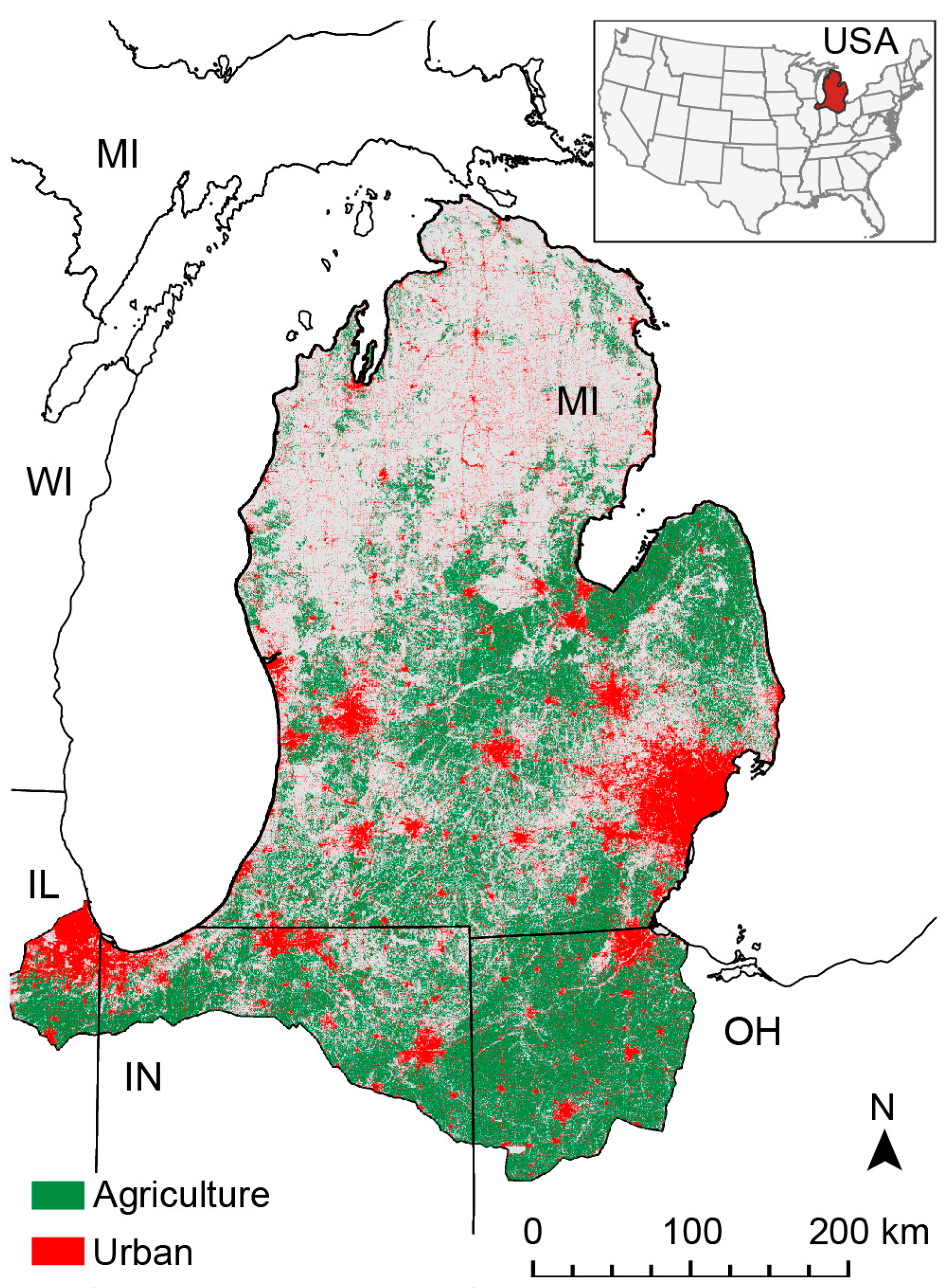
2.1. Study Area
2.2. Data
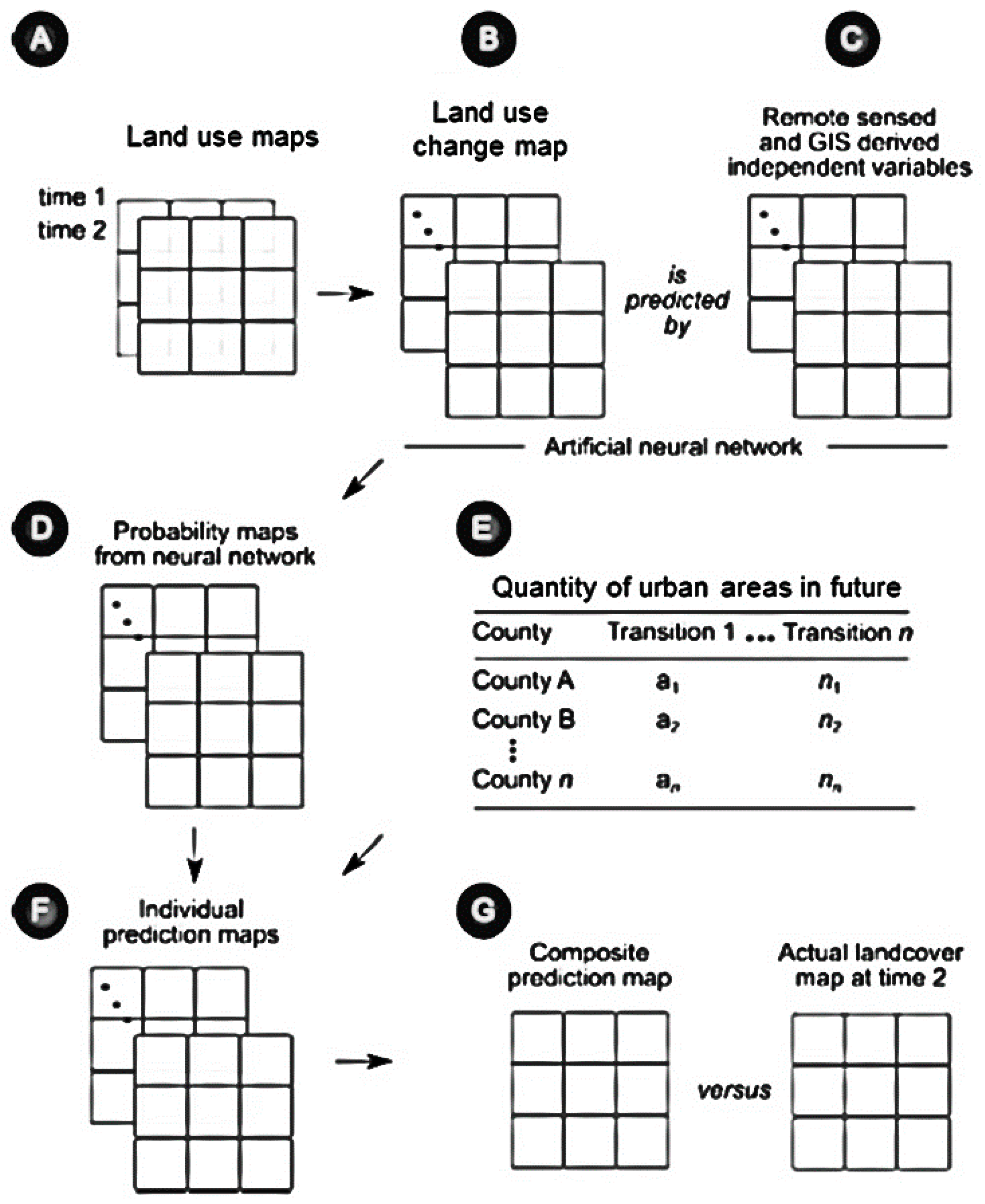
2.3. Land Transformation Model
2.4. Model Calibration
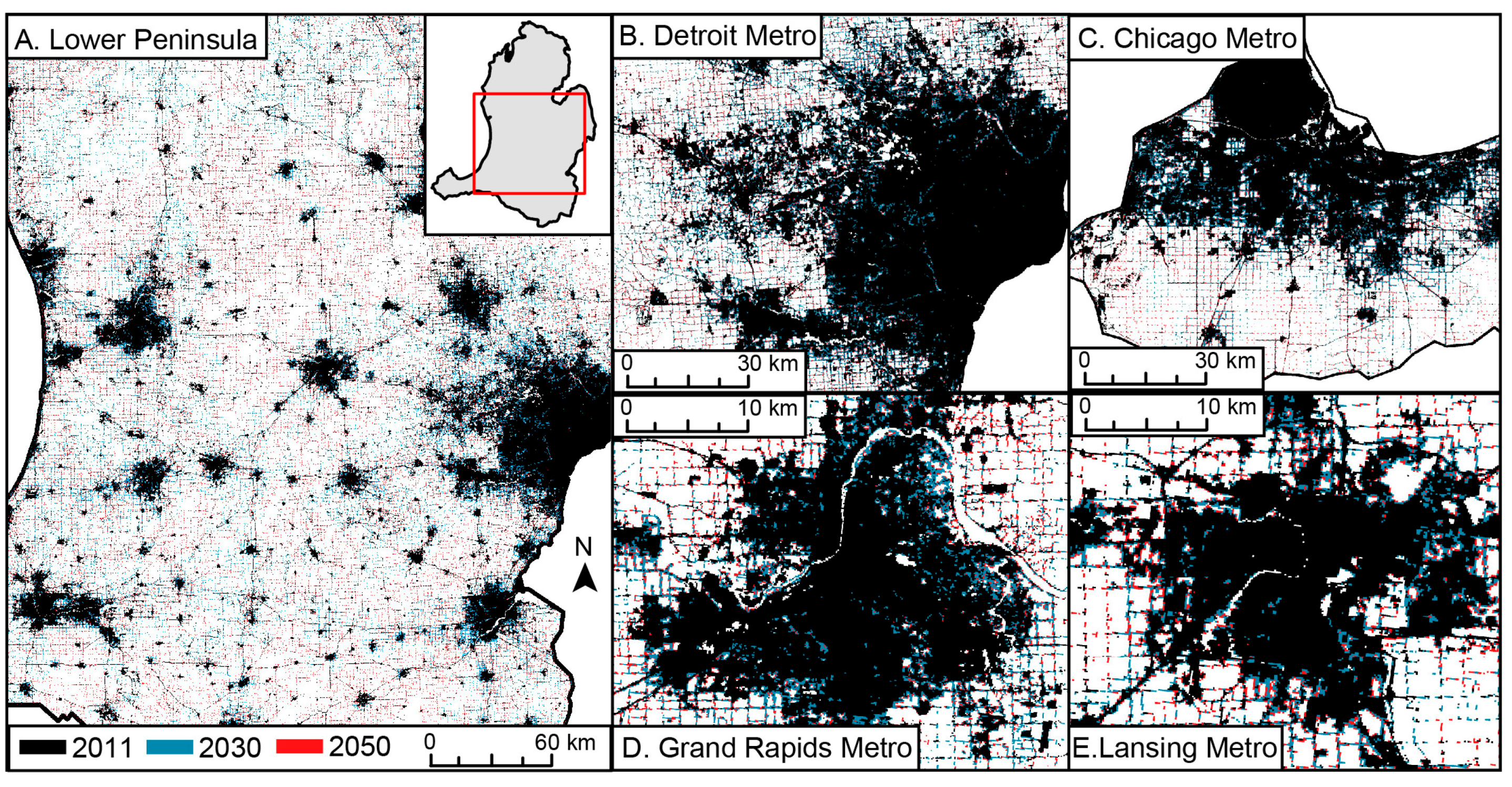
2.5. Future Land Cover Projection
3. Conclusions
Author Contributions
Conflicts of Interest
References
- Pijanowski, B.C.; Tayyebi, A.; Doucette, J.; Pekin, B.K.; Braun, D.; Plourde, J. A big data urban growth simulation at a national scale: Configuring the GIS and neural network based land transformation model to run in a high performance computing (HPC) environment. Environ. Model. Softw. 2014, 51, 250–268. [Google Scholar] [CrossRef]
- Tayyebi, A.; Pekin, B.K.; Pijanowski, B.C.; Plourde, J.D.; Doucette, J.S.; Braun, D. Hierarchical modeling of urban growth across the conterminous USA: Developing meso-scale quantity drivers for the Land Transformation Model. J. Land Use Sci. 2013, 8, 422–442. [Google Scholar] [CrossRef]
- Grimm, N.B.; Faeth, S.H.; Golubiewski, N.E.; Redman, C.L.; Wu, J.; Bai, X.; Briggs, J.M. Global change and the ecology of cities. Science 2008, 319, 756–760. [Google Scholar] [CrossRef] [PubMed]
- Fifth Global Environment Outlook: Environment for the Future We Want; UNEP: Geneva, Switzerland, 2012.
- Tayyebi, A.; Meehan, T.D.; Dischler, J.; Radloff, G.; Ferris, M.; Gratton, C. SmartScape™: A web-based decision support system for assessing the tradeoffs among multiple ecosystem services under crop-change scenarios. Comput. Electron. Agric. 2016, 121, 108–121. [Google Scholar] [CrossRef]
- Meehan, T.D.; Gratton, C.; Diehl, E.; Hunt, N.D.; Mooney, D.F.; Ventura, S.J.; Jackson, R.D. Ecosystem-service tradeoffs associated with switching from annual to perennial energy crops in riparian zones of the US Midwest. PLoS ONE 2013, 8, e80093. [Google Scholar] [CrossRef] [PubMed]
- Kalnay, E.; Cai, M. Impact of urbanization and land-use change on climate. Nature 2003, 423, 528–531. [Google Scholar] [CrossRef] [PubMed]
- Rudel, T.K.; Coomes, O.T.; Moran, E.; Achard, F.; Angelsen, A.; Xu, J.; Lambin, E. Forest transitions: Towards a global understanding of land use change. Glob. Environ. Chang. 2005, 15, 23–31. [Google Scholar] [CrossRef]
- Searchinger, T.; Heimlich, R.; Houghton, R.A.; Dong, F.; Elobeid, A.; Fabiosa, J.; Yu, T.H. Use of US croplands for biofuels increases greenhouse gases through emissions from land-use change. Science 2008, 319, 1238–1240. [Google Scholar] [CrossRef] [PubMed]
- Lambin, E.F.; Meyfroidt, P. Global land use change, economic globalization, and the looming land scarcity. Proc. Natl. Acad. Sci. USA 2001, 108, 3465–3472. [Google Scholar] [CrossRef] [PubMed]
- Baker, A. Land Use and Water Quality. In Encyclopedia of Hydrological Sciences; John Wiley and Sons, Inc.: Hoboken, NJ, USA, 2005. [Google Scholar]
- Schneider, A.; Friedl, M.A.; Potere, D. A new map of global urban extent from MODIS satellite data. Environ. Res. Lett. 2009, 4, 044003. [Google Scholar] [CrossRef]
- Homer, C.H.; Fry, J.A.; Barnes, C.A. The national land cover database. US Geol. Surv. Fact Sheet 2012, 3020, 1–4. [Google Scholar]
- Belward, A.S.; Estes, J.E.; Kline, K.D. The IGBP-DIS global 1-km land-cover data set DISCover: A project overview. Photogramm. Eng. Remote Sens. 1999, 65, 1013–1020. [Google Scholar]
- Cover, G.L. v2 2008 database. 2008. [Google Scholar]
- Arsanjani, J.J.; See, L.; Tayyebi, A. Assessing the suitability of GlobeLand30 for mapping land cover in Germany. Int. J. Digit. Earth 2016, 9, 1–19. [Google Scholar] [CrossRef]
- Arsanjani, J.J.; Tayyebi, A.; Vaz, E. GlobeLand30 as an alternative fine-scale global land cover map: Challenges, possibilities, and implications for developing countries. Habitat Int. 2016, 55, 25–31. [Google Scholar] [CrossRef]
- Ostrom, E. A general framework for analyzing sustainability of social-ecological systems. Science 2009, 325, 419–422. [Google Scholar] [CrossRef] [PubMed]
- López, E.; Bocco, G.; Mendoza, M.; Duhau, E. Predicting land-cover and land-use change in the urban fringe: A case in Morelia city, Mexico. Landsc. Urban Plan. 2001, 55, 271–285. [Google Scholar] [CrossRef]
- Pijanowski, B.C.; Tayyebi, A.; Delavar, M.R.; Yazdanpanah, M.J. Urban expansion simulation using geospatial information system and artificial neural networks. Int. J. Environ. Res. 2010, 3, 493–502. [Google Scholar]
- Lambin, E.F.; Turner, B.L.; Geist, H.J.; Agbola, S.B.; Angelsen, A.; Bruce, J.W.; George, P. The causes of land-use and land-cover change: Moving beyond the myths. Glob. Environ. Chang. 2001, 11, 261–269. [Google Scholar] [CrossRef]
- Verburg, P.H.; Overmars, K.P. Combining top-down and bottom-up dynamics in land use modeling: Exploring the future of abandoned farmlands in Europe with the Dyna-CLUE model. Landsc. Ecol. 2009, 24, 1167–1181. [Google Scholar] [CrossRef]
- Tayyebi, A.; Pijanowski, B.C.; Linderman, M.; Gratton, C. Comparing three global parametric and local non-parametric models to simulate land use change in diverse areas of the world. Environ. Model. Softw. 2014, 59, 202–221. [Google Scholar] [CrossRef]
- McMillen, D.P. An empirical model of urban fringe land use. Land Econ. 1989, 65, 138–145. [Google Scholar] [CrossRef]
- Clarke, K.C.; Hoppen, S.; Gaydos, L. A self-modifying cellular automaton model of historical urbanization in the San Francisco Bay area. Environ. Plan. B 1997, 24, 247–261. [Google Scholar] [CrossRef]
- Tayyebi, A.; Pijanowski, B.C.; Pekin, B. Two rule-based urban growth boundary models applied to the Tehran Metropolitan Area, Iran. Appl. Geogr. 2011, 31, 908–918. [Google Scholar] [CrossRef]
- Parker, D.C.; Manson, S.M.; Janssen, M.A.; Hoffmann, M.J.; Deadman, P. Multi-agent systems for the simulation of land-use and land-cover change: A review. Ann. Assoc. Am. Geogr. 2003, 93, 314–337. [Google Scholar] [CrossRef]
- Tayyebi, A.; Pijanowski, B.C. Modeling multiple land use changes using ANN, CART and MARS: Comparing tradeoffs in goodness of fit and explanatory power of data mining tools. Int. J. Appl. Earth Obs. Geoinf. 2014, 28, 102–116. [Google Scholar] [CrossRef]
- Pijanowski, B.C.; Brown, D.G.; Shellito, B.A.; Manik, G.A. Using neural networks and GIS to forecast land use changes: A land transformation model. Comput. Environ. Urban Syst. 2002, 26, 553–575. [Google Scholar] [CrossRef]
- Pijanowski, B.C.; Alexandridis, K.T.; Mueller, D. Modelling urbanization patterns in two diverse regions of the world. J. Land Use Sci. 2006, 1, 83–108. [Google Scholar] [CrossRef]
- Tayyebi, A.; Tayyebi, A.H.; Arsanjani, J.J.; Moghadam, H.S.; Omrani, H. FSAUA: A framework for sensitivity analysis and uncertainty assessment in historical and forecasted land use maps. Environ. Model. Softw. 2016, 84, 70–84. [Google Scholar] [CrossRef]
- Ray, D.K.; Pijanowski, B.C.; Kendall, A.D.; Hyndman, D.W. Coupling land use and groundwater models to map land use legacies: Assessment of model uncertainties relevant to land use planning. Appl. Geogr. 2012, 34, 356–370. [Google Scholar] [CrossRef]
- Olson, J.M.; Alagarswamy, G.; Andresen, J.A.; Campbell, D.J.; Davis, A.Y.; Ge, J.; Pijanowski, B.C. Integrating diverse methods to understand climate–land interactions in East Africa. Geoforum 2008, 39, 898–911. [Google Scholar] [CrossRef]
- Tayyebi, A.; Jenerette, G.D. Increases in the climate change adaption effectiveness and availability of vegetation across a coastal to desert climate gradient in metropolitan Los Angeles, CA, USA. Sci. Total Environ. 2016, 548, 60–71. [Google Scholar] [CrossRef] [PubMed]
- Pijanowski, B.; Ray, D.K.; Kendall, A.D.; Duckles, J.M.; Hyndman, D.W. Using backcast land-use change and groundwater travel-time models to generate land-use legacy maps for watershed management. Ecol. Soc. 2007, 12, 25. [Google Scholar] [CrossRef]
- Azari, M.; Tayyebi, A.; Helbich, M.; Reveshty, M.A. Integrating cellular automata, artificial neural network, and fuzzy set theory to simulate threatened orchards: Application to Maragheh, Iran. GIScience Remote Sens. 2016, 53, 183–205. [Google Scholar] [CrossRef]
- Shafizadeh-Moghadam, H.; Asghari, A.; Tayyebi, A.; Taleai, M. Coupling machine learning, tree-based and statistical models with cellular automata to simulate urban growth. Comput. Environ. Urban Syst. 2017, 64, 297–308. [Google Scholar] [CrossRef]
- DeNavas-Walt, C.; Proctor, B.D.; Smith, J.C. Income, Poverty, and Health Insurance Coverage in the United States: 2009; US Census Bureau, current population reports, P60-238; U.S. Government Printing Office: Washington, DC, USA, 2010.
- Song, W.; Pijanowski, B.C.; Tayyebi, A. Urban expansion and its consumption of high-quality farmland in Beijing, China. Ecol. Indic. 2015, 54, 60–70. [Google Scholar] [CrossRef]
- Shafizadeh-Moghadam, H.; Asghari, A.; Taleai, M.; Helbich, M.; Tayyebi, A. Sensitivity analysis and accuracy assessment of the land transformation model using cellular automata. GIScience Remote Sens. 2017, 1–18. [Google Scholar] [CrossRef]
- Newman, G.; Lee, J.; Berke, P. Using the land transformation model to forecast vacant land. J. Land Use Sci. 2016, 11, 450–475. [Google Scholar] [CrossRef]
- Tayyebi, A.H.; Delavar, M.R.; Tayyebi, A.; Golobi, M. Combining multi criteria decision making and Dempster Shafer theory for landfill site selection. Int. Arch. Photogramm. Remote Sens. Spat. Inf. Sci. 2010, 38, 6. [Google Scholar]
- Pontius, R.G., Jr.; Batchu, K. Using the relative operating characteristic to quantify certainty in prediction of location of land cover change in India. Trans. GIS 2003, 7, 467–484. [Google Scholar] [CrossRef]


| Year | Chicago | Detroit | Grand Rapids | Kalamazoo | Lansing | Saginaw | South Bend | Toledo | Traverse City |
|---|---|---|---|---|---|---|---|---|---|
| 2011 | 21.31 | 39.35 | 7.84 | 2.47 | 3.57 | 2.14 | 7.25 | 5.97 | 1.12 |
| 2015 | 23.43 | 42.54 | 8.59 | 2.77 | 3.88 | 2.27 | 7.68 | 6.56 | 1.20 |
| 2020 | 24.39 | 44.10 | 9.06 | 2.96 | 4.07 | 2.34 | 8.01 | 6.94 | 1.43 |
| 2025 | 24.88 | 45.05 | 9.39 | 3.07 | 4.22 | 2.43 | 8.24 | 7.17 | 1.50 |
| 2030 | 25.30 | 45.76 | 9.66 | 3.13 | 4.32 | 2.52 | 8.44 | 7.37 | 1.52 |
| 2035 | 25.79 | 46.44 | 9.96 | 3.21 | 4.43 | 2.60 | 8.59 | 7.57 | 1.58 |
| 2040 | 26.25 | 47.17 | 10.15 | 3.30 | 4.53 | 2.67 | 8.74 | 7.81 | 1.72 |
| 2045 | 26.60 | 47.84 | 10.36 | 3.38 | 4.62 | 2.72 | 8.94 | 7.99 | 1.84 |
| 2050 | 26.93 | 48.42 | 10.58 | 3.43 | 4.75 | 2.79 | 9.10 | 8.14 | 1.94 |
© 2017 by the authors. Licensee MDPI, Basel, Switzerland. This article is an open access article distributed under the terms and conditions of the Creative Commons Attribution (CC BY) license (http://creativecommons.org/licenses/by/4.0/).
Share and Cite
Tayyebi, A.; Smidt, S.J.; Pijanowski, B.C. Long-Term Land Cover Data for the Lower Peninsula of Michigan, 2010–2050. Data 2017, 2, 16. https://doi.org/10.3390/data2020016
Tayyebi A, Smidt SJ, Pijanowski BC. Long-Term Land Cover Data for the Lower Peninsula of Michigan, 2010–2050. Data. 2017; 2(2):16. https://doi.org/10.3390/data2020016
Chicago/Turabian StyleTayyebi, Amin, Samuel J. Smidt, and Bryan C. Pijanowski. 2017. "Long-Term Land Cover Data for the Lower Peninsula of Michigan, 2010–2050" Data 2, no. 2: 16. https://doi.org/10.3390/data2020016
APA StyleTayyebi, A., Smidt, S. J., & Pijanowski, B. C. (2017). Long-Term Land Cover Data for the Lower Peninsula of Michigan, 2010–2050. Data, 2(2), 16. https://doi.org/10.3390/data2020016