Adaptive Degradation Prognostic Reasoning by Particle Filter with a Neural Network Degradation Model for Turbofan Jet Engine


1
IVHM Centre, Cranfield University, Bedford MK43 0AL, UK
2
Artesis, 41480 Gebze, Kocaeli, Turkey
3
College of Engineering, Taibah University, Al-Medina Al-Munawara, Medina 42353, Saudi Arabia
*
Author to whom correspondence should be addressed.
Data 2018, 3(4), 49; https://doi.org/10.3390/data3040049
Submission received: 27 September 2018
/
Revised: 30 October 2018
/
Accepted: 1 November 2018
/
Published: 6 November 2018
Abstract
:In the aerospace industry, every minute of downtime because of equipment failure impacts operations significantly. Therefore, efficient maintenance, repair and overhaul processes to aid maximum equipment availability are essential. However, scheduled maintenance is costly and does not track the degradation of the equipment which could result in unexpected failure of the equipment. Prognostic Health Management (PHM) provides techniques to monitor the precise degradation of the equipment along with cost-effective reliability. This article presents an adaptive data-driven prognostics reasoning approach. An engineering case study of Turbofan Jet Engine has been used to demonstrate the prognostic reasoning approach. The emphasis of this article is on an adaptive data-driven degradation model and how to improve the remaining useful life (RUL) prediction performance in condition monitoring of a Turbofan Jet Engine. The RUL prediction results show low prediction errors regardless of operating conditions, which contrasts with a conventional data-driven model (a non-parameterised Neural Network model) where prediction errors increase as operating conditions deviate from the nominal condition. In this article, the Neural Network has been used to build the Nominal model and Particle Filter has been used to track the present degradation along with degradation parameter.
1. Introduction
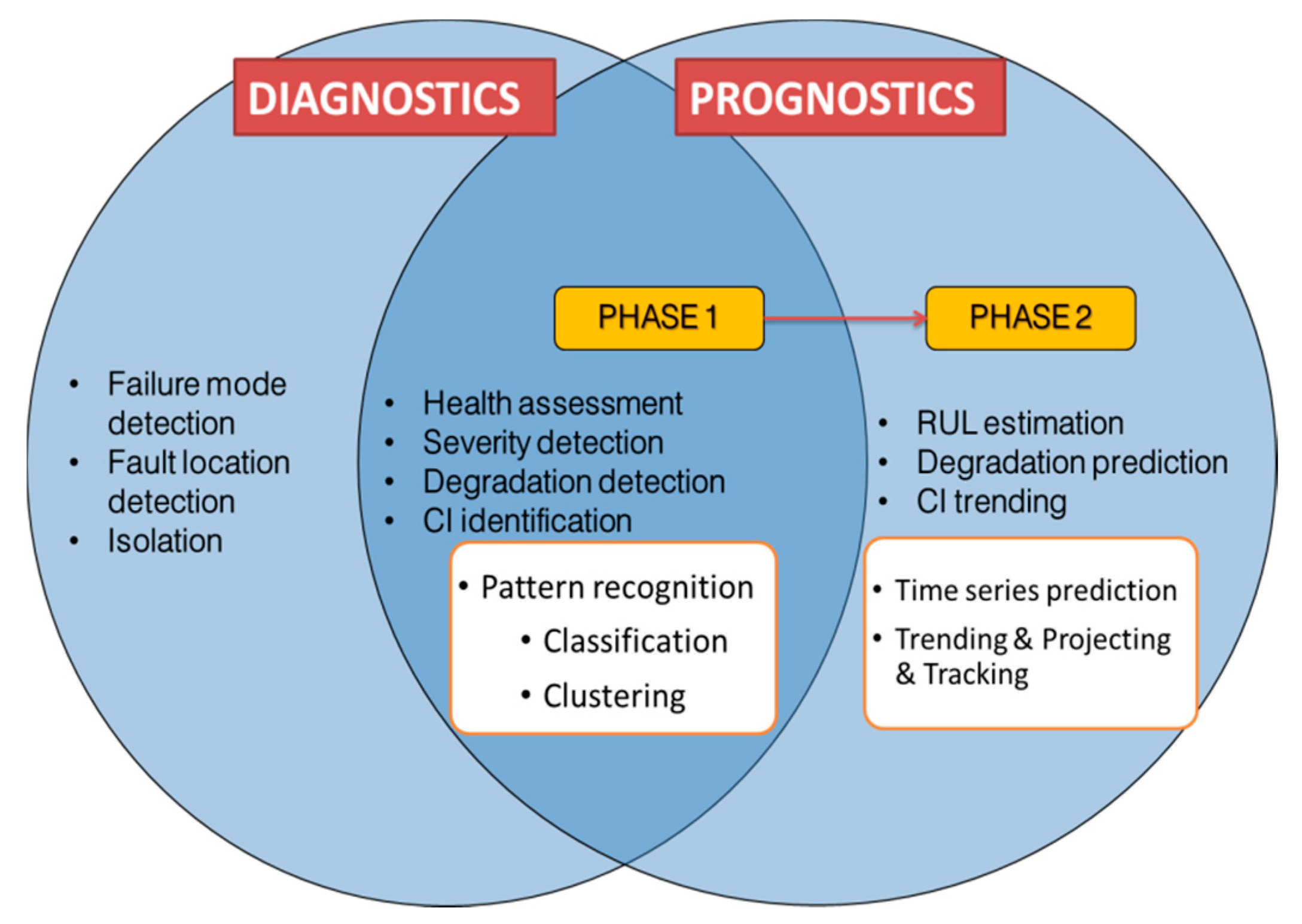
Integrated Vehicle Health Management (IVHM) is a relatively new comprehensive maintenance technology, enabling many disciplines with an integrated framework. Maintenance strategies such as Condition Based Maintenance (CBM) or Reliability-Centered Maintenance (RCM) are offered within the IVHM framework. The prognostics and diagnostics are both integrated in CBM and Predictive Maintenance. Such strategies involve monitoring of sensory information and studying the possible future health level of the system based on the monitored data [1]. The scope of diagnostics and prognostics in IVHM is shown in the Figure 1.
IVHM technology has potential applications in many fields, such as aerospace, military systems, electronics, machinery, energy and manufacturing. IVHM is a major component in a new future asset management, where a conscious effort is made to shift asset maintenance from a scheduled-based approach to a more proactive and predictive approach [3]. Its goal is to maximize asset operational availability while minimizing downtime and the logistics footprint through monitoring deterioration of component conditions. IVHM involves data processing which comprehensively consists of capturing data related to assets, monitoring parameters, assessing current or future health conditions through prognostics and providing recommended maintenance actions.
Prognostics is challenging and the fundamental technology within IVHM, where it requires identification of the current health level and extrapolating it to a predefined failure threshold, concluded with the estimation of remaining useful life (RUL). The output of prognostics (i.e., RUL) is the duration between the current time and the time at which the forecast health level reaches a predefined threshold, i.e., the amount of time the equipment will continue to perform its function according to design specifications [4]. Benefits of the prognostics motivate researchers and the industry to achieve reduced costs, increased safety and availability via better maintenance planning.
An engine is the most critical system in any aircraft, the safety of the aircraft engine has to be considered as the most important in aircraft life cycle. The failure of an engine could lead to an aircraft returning to ground if not a catastrophic accident. In an economic terms, this means a significant cost to an aircraft operator. Therefore, this article focuses on prognostics prediction of the turbofan jet engine.
2. Background
The prognostics prediction of the jet engine is a very daunting task as there are many different sensors involved and physical degradation of the engines is very complex. A number of sensors of varying types may be mounted in the engine, to sense several physical parameters (for example, combustion temperature, vibration, pressure at different levels, etc.) and monitoring the aircraft engine system’s functional and environmental conditions associated with engine operation. Therefore, there is demand to develop methods that utilise the aircraft system’s health conditions to detect aircraft engine performance degradation, faults, and the remaining useful life (RUL) prediction.
In prognostics, commonly used approaches are ‘Data-Driven’ and ‘Model-Based’ (some use the term ‘Physics-Based’). Many engineering applications of the data-driven approach are reported in literature. Neural Network (NN) (including its variants) is one of the most popular data-driven techniques and has been used in remaining useful life (RUL) predictions for a manufacturing machine tool [5,6], bearing of a rotating machine [7] and electro-mechanical actuator of F/A-18 aircraft’s stabilizer [8,9] compares the difference between Neural Network and linear regression (or trending) in the context of prognostics. In addition to Neural Network, Support Vector Regression (SVR) is another nonlinear regression technique which has been applied in bearing life prediction of a manufacturing machine [10,11]. A Hidden Markov Model (HMM) is a data-driven approach where a degradation profile is discretized into states evolved based on either non- or time dependent transition probability. Its application in bearing life prognostics is reported in [12,13]. In contrast to NN, SVR and HMM where models are trained offline, Gaussian Process (GP) is an online data-driven technique where a degradation model is learned from the data being rendered. In GP, a future remaining profile is assumed to follow the same degradation dynamics as the model which is trained up to the specified data point. GP has been applied to predict state-of-charge and state-of-health of a lithium-ion battery [14] and crack length propagation of a composite material [15]. The other data-driven prognostic approach that is worth mentioning is to base it on a statistical (or stochastic) process model. Its comprehensive review can be found in [16,17].
In the model-based approach, model parameters have explicit physical meanings, in which an online parameter estimation algorithm can be used to estimate or learn those parameters that are contributing to the degradation. Kalman Filter (KF) and Particle Filter (PF) are such estimation algorithms that are commonly used in model-based prognostics. KF is restricted to a linear and higher-order Taylor series-based model. KF has been applied on a Paris’s model to predict bearing life of a rotating machine [18] and on state-of-charge model to predict RUL of a lithium-ion battery [19]. PF is a more generalized version of KF which is applicable to a nonlinear degradation model with non- or Gaussian uncertainties. Examples of PF used in prognostics are in prediction of crack length propagation of a material [4], degradation of a centrifugal pump [20] and response time of a pneumatic valve [21]. Physics of failure (PoF) is another model-based approach where operating cycles available of a component is estimated based on parameters related to operating condition [22]. PoF has its route from reliability engineering. Examples of the PoF model are corrosion-fatigue mechanism of a material [23] and a gas turbine blade integrated with predictive maintenance scheme [24].
However, the data-driven and model-based prognostic approaches are by no means without their own limitations. The data-driven approach is restricted to a known narrow range of operating conditions. The model-based approach on the other hand has its limitations in terms of derivation of a physical degradation model which can be infeasible for the case of complex degradation mechanisms. Until now, there have been very few prognostic examples addressing both shortcomings reported in the literature. Therefore, a prognostic approach that allows a complex degradation profile to be accurately modelled and is able to be adaptive to a wide range of operating profiles, which is likely to be the case in practice, would be of particular interest. In this paper, we explore how a complex degradation profile, where a traceable physical model might not be feasible, is modelled and adapted to a variation of operating profiles. This and how the developed model is used with an online parameter estimator in prognostics will be the contribution of this paper. In this study, a turbofan jet engine data is used as an engineering application to demonstrate proof-of-concept of the proposed approach.
Diagnostics and Prognostics for Turbine Engine
Gas turbine performance and degradation calculation is a daunting task. The system-level performance deterioration is a main cause of concern for system reliability, availability, and operating costs. To identify the current as well as the future health state of a deteriorating engine is a key factor for ensuring reliable operation and optimal usage.
Deterioration of gas turbine engines while in service results from a number of complex physical mechanisms, and the methods of predicting deterioration of an engine have been discussed in different ways [25,26,27,28,29].
The gas turbine deterioration phenomenon is so complicated that no single prognostic approach can cover all scenarios. To make the approach proposed in this study applicable, we assume that the regular on-line maintenance actions do not change the engine degradation pattern and that the engine operates under a regular usage profile, which is common practice in modern commercial aviation [25]. The overall performance deterioration patterns of gas turbine engines under such a common usage profile have been studied in the literature. One of the typical deterioration patterns is the combined pattern. In this case, the engine degrades linearly with a constant degradation rate during the first period of operation, which is then followed by an increasing degradation rate during the second period of operation [25]. Saxena and Goebel have proposed an exponential model for modelling damage propagation for engine degradation simulation [26]. Another typical engine performance deterioration model is described in [27,28], where a deterioration formula of y = a√t + b is proposed. Here a and b are the parameters to be determined. No consensus has been reached on this topic, and engine performance may degrade depending on the actual operating conditions.
A more flexible degradation modelling technique is needed for practical applications. In practice, faults or abnormal operation may cause an irreversible sudden drop in performance, introducing change points or structural breaks into the degradation model.
In 2007, Wang et al. presented a conceptual system for remote monitoring and fault diagnosis of gas turbine-based power generation systems, where gas turbines are similar to turbofan jet engines in some aspects [30]. In this research, Wang et al. focus on normalising the data in a way that the operating conditions have no influence on the RUL estimates, which is the major draw-back of the data-driven techniques. This article addresses this issue and presents the technique which take operating condition into account and then predicts the RUL rather than using normalised model.
In 2008, Donat et al. discussed the issues of data visualization, data reduction, and ensemble learning for intelligent fault diagnosis in gas turbine engines [31].
In 2009, Li and Nilkitsaranont described a prognostic approach to estimating the remaining useful life of gas turbine engines before their next major overhaul based on a combined regression technique with both linear and quadratic models [25]. In the same year, Bassily et al. proposed a technique, which assessed whether or not the multivariate auto covariance functions of two independently sampled signals coincide, to detect faults in a gas turbine [32].
In 2010, Young et al. presented an offline fault diagnosis method for industrial gas turbines in a steady-state using Bayesian data analysis. The authors employed multiple Bayesian models via model averaging for improving the performance of the resulted system [33].
In 2011, Yu et al. designed a sensor fault diagnosis technique for Micro-Gas Turbine Engine based on wavelet entropy, where wavelet decomposition was utilized to decompose the signal in different scales, and then the instantaneous wavelet energy entropy and instantaneous wavelet singular entropy are computed based on the previous wavelet entropy theory [34].
In 2012, Wu et al. studied the issue of bearing fault diagnosis based on multi-scale permutation entropy and support vector machine [35]. In 2013, Wu et al. designed a technique for defecting diagnostics based on multi-scale analysis and support vector machines [36]. However, the degradation of turbofans like jet engines depends on the operating conditions as the operating condition changes, the degradation pattern changes. In the literature, most of the techniques used to calculate RUL are presented on a similar pattern of degradation. Therefore, if the condition changes the calculation of RUL does not provide very accurate results. The physical based models are more appropriate in such cases. Nevertheless, to create a physical model for complex systems such as a turbofan would be very difficult. To solve this problem, this article presents an adaptive data-driven technique, the details of the technique are discussed later in this article.
3. Proposed Approach
The framework of prognostics needs to be developed which could be adaptable to the present conditions of the system. This prognostics framework could identify causal links between precursors and their associated system health indices in the form that will be relevant to the alert/alarm generation, operation and further predictive trend analysis. A framework which could make sensor data into meaningful information would be a quantitative value like probability, certainty or likelihood of an event or combination events will compromise the safety margin or cause a particular impact on operation.
The requirement of the dataset was that it had to be real or accurate, therefore, the NASA turbofan data set has been used to for this reasoning system.
NASA Turbofan Dataset
The dataset given in [29] consists of multivariate time series signals that are collected from the turbofan engine dynamic simulation process. The engine run-to-failure simulations were carried out using C-MAPSS, a well-known simulation program for transient operation of modern commercial turbofan engines. A hundred engine’s run-to-failure time series trajectories are considered in this study (dataset FD001) which can be considered to form a fleet of engines of the same type. The aircraft gas turbine engine’s RUL is closely bound up with its conditions. To monitor the aircraft gas turbine engines conditions, several kinds of signals could be used such as temperature, pressure speed and air ratio. In this simulation a total of 21 sensors were installed in the aircraft engine’s different components (Fan, LPC, HPC, LPT, HPT, Combustor and Nozzle) to monitor the aircraft engine’s health conditions. The 21 sensory signals, as detailed in the Table 1 below, where obtained from the above-mentioned sensors. Among the 21 sensory signals, some signals contain little or no degradation information whereas the other signalises a degradations trend. Most of the sensors data were contaminated with measurement noise.
To improve the RUL prediction accuracy and efficiency, important sensory signals must be carefully selected to characterize degradation behaviour for the aircraft gas turbine engine health prognostics. The sensors which were selected must be better in prognosibility and trendability. By observing the degradation behaviour of the 21 sensory signals, seven of them (2, 4, 7, 8, 11, 12, and 15) were selected in this study by the guide of naked eye examination of the degradation trends.
The engine run-to-failure simulations were carried out using C-MAPSS, are presentative simulation model of a modern commercial turbofan engine [37].
C-MAPSS have 14 inputs and 13 health parameters which enable the user to simulate the effects of faults and deterioration in any of the five rotating components of the engine (fan, LPC, HPC, HPT, and LPT). C-MAPSS can produce 58 different outputs, e.g., the various performance measurements typically available from aircraft gas turbine engines as well as operability margins.
The time series of sensor measurements is recorded to characterize the evolution of the concealed health state of the engine simulated. Figure 2 shows the basic jet engine design of the C-MAPSS simulation. Each record, a 24-element vector, consists of three values for the operational settings and 21 values for engine performance measurements, which are contaminated with noise to simulate the real engine more precisely.
The operability margins, such as stall and temperature margins, define the safe operation region for the engine. Six different flight conditions were simulated, comprising arrange of values for three operational settings: altitude (Alt: 0–42 Kft), Mach number (M: 0–0.84), and throttle solver angle (TRA: 20–100). Each engine degradation simulation starts with a different initial degradation state due to different degrees of initial wear and manufacturing variation in practice. In this study, snapshots of engine performance parameters at sea level for each flight were used, i.e., Alt = 0, M = 0, and TRA = 100). For more details on the engine run-to-failure simulation, the reader is referred to [26]. Readers are suggested to find the detailed information regarding the sensory signal screening from [29].
4. Reasoning and Prediction through Health Index Calculation
4.1. Health Index
The Health Index (HI) term is defined by a discrete number representing the actual health of the system. For instance, 1 indicates the best health condition and 0 signifies the worst health condition. A mid-range value such as 0.5 represents half-life. The virtual health index of the system can be calculated in this system by using of the following formula:
In this article, we formulized the health index at a specific time point as the rate of current RUL (Remaining Useful Life) to the End-of-Life (EoL) of the system.
The Figure 3 above shows the linear HI index calculated from the initial state of the system as the HI is calculated from the Equation (1). However, when the sensor readings are received the HI calculation will be dynamic according to the sensor data received.
The above Figure 4 shows the HI on the Y-axis and the sensor reading on the X-axis. This Figure shows the degradation of a sub-system; as the subsystem health degrades with time the health index will decrease. The red outbound also provides the uncertainty of the calculation. In real life the health of the system degrades in similar way, in otherward the Figure 4 shows the health degradation as a linear line, is not real behaviour of health degradation. The details of HI calculation have been discussed later in this article along with the presented technique.
4.2. Motivation
Particle filters (PF) are commonly used Bayesian estimators for tracking the state of a degrading system. The common usage involves tracking the parameters of the state transition equation as well as tracking the main degradation indicator (i.e., health index). In many systems the degradation health index is measured via a sensor which means the sensor provides direct condition monitoring data.
However, the sensory data brings the noise as well as accuracy problems with it. Therefore, PF are used to estimate the actual state of the system behaviour which is the actual response supposed to be measured.
On the other hand, for the cases where the actual health index of the system is not directly measured (i.e., indirect CM), the health index is approximated via transforming the sensory information. The sensory information does not directly exhibit the health of the component/system however, it shows a degradation profile to be used in the transformation process.
The engine degradation simulation data has health index information, however, the dataset suppliers (NASA) did not provide HI degradation information. The information NASA provide is the operational profiles and the sensory data corresponding to some components. Therefore, one has to establish a mechanism which transforms the sensory data into the health index to be used with particle filters.
It is a known phenomenon that constructing a physics-based degradation model for complex systems like a jet engine is extremely complex and difficult. However, the dynamic system state transition model can be approximated using regression or machine learning algorithms. The complexity of modelling the degradation behaviour is achieved by the learning algorithm which maps the sensory data into HI. However, the approximated data-driven nominal state transition model is not adaptable for different profiles of data.
The data-driven techniques are not adaptable; basically, NASA provide a dynamic model with fixed parameters. For example, consider a spring system whose physical equation is . However, in a data-driven model like neural network is embedded in the neurons and weights. These weights and neurons are fixed and cannot be changed, where in the physical spring model if you change ‘k’ the behaviour of the model will be changed. Therefore, for machine learning and data-driven models you simply cannot change the behaviour of the model so their models are not adaptable.
The primary novelty of this research is that it provides the adaptable data-driven technique which mainly captures different operational profiles. The secondary novelty of this work is to transform the RUL information into HI as well as mapping the sensory data to HI values using a machine learning algorithm (i.e., NN) to be used as a measurement function within the particle filter tracking mechanism. In this way, the nominal mapping algorithm results are becoming adaptable by taking into account the particle filters which leads to more accurate prognostic results. The details of the methodology are elaborated in next section.
4.3. Health Index Modelling Using Neural Network
Radial basis functions (RBF) are kind of neural networks used for function approximations. RBFs are usually used in time series predictions, forecasting problems, regression, classification, non-linear system control etc. RBFs are three-layer feed-forward neural networks, where the hidden nodes implement a set of radial basis functions (e.g., Gaussian functions) as shown in Figure 5. On the other hand, the output nodes implement linear summation functions as in Multi-Layer Perceptron (MLP). The approximation function can be described in the following form in Equation (2):
where, represents the actual approximation function with numbers of radial basis. Each basis function is associated with different centres. Centre mean and standard deviation is symbolised as ‘’ along with the associated weights ‘’. ‘’ in the equation stands for the measurement inputted in the system. The norm and the basis function (i.e., ‘’) are typically taken to be the Euclidean distance respectively. In this research the Gaussian basis function is selected. Gaussian basis function can be formulised as given in Equation (3):
RBF networks are universal approximators. This means that a RBF network with enough hidden neurons can approximate any continuous function with arbitrary precision. The weights ‘’ and ‘’ are determined in a manner that optimizes the fit between the output and input.
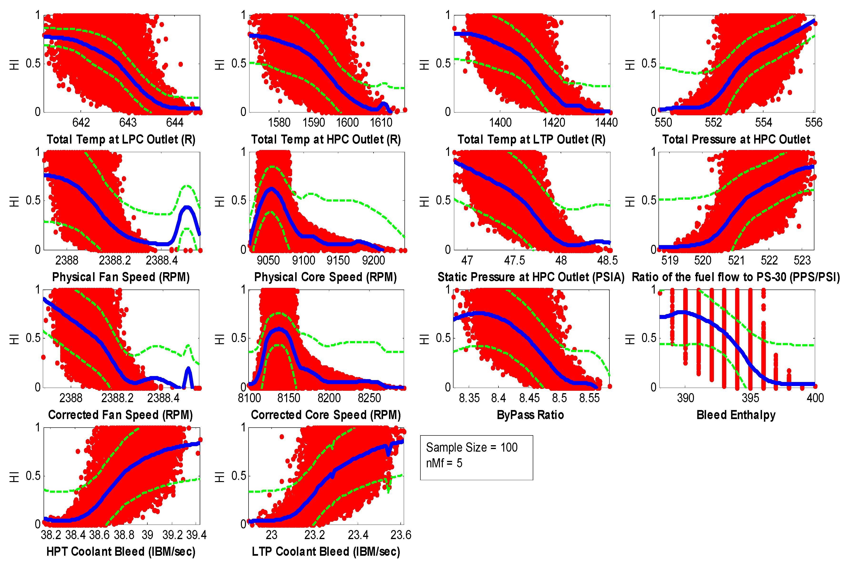
The Neural Network has been fed with the sensor data and been mapped to the HI index along with the bound confidence (standard deviation) of 30%. The RBF also calculates and maps the data to the probability level because, normal NN does not provide the probability/confidence levels. The outputs of the RBF of the entire sensors are shown in Figure 5. The Figure shows the basic architecture of the Neural Network with the RBF function used. There are two inputs and two outputs to the NN, one output is the nominal model and the other is the standard deviation of the nominal model. This model has been fed the data from the NASA trouble fan which has been mentioned in the previous section. Furthermore, 70% of the data has been used to train the NN model and 30% of the data has been used to test the presented technique.
Cost Function
In the previous section, Neural Network modelling is explained. However, for the model to closely approximate the degradation process, the model parameter values need to be tuned (or system identified) from the collected data samples. The aim is to minimize/optimize the prediction errors between the experimental degradation data and simulated data from the NN model.
The centres and associated weights are determined using a constrained nonlinear optimisation algorithm (i.e., ‘fmincon’) provided within MatLab. To do that, an object function script is written to calculate the error regarding the optimisation output.
In this paper, Maximum likelihood Estimation () is used as a performance measure for system identification of the Neural Network degradation model defined in (Equation (2)). For a given data sample, is obtained by maximising the log-likelihood metric, which is given in Equation (4):
where ‘’ and ‘’ are the basis function centre mean and standard deviation, whereas ‘’ is the input measurement from the training data.
5. Particle Filter
5.1. Probabilistic Model
In order to predict of a system, the system’s current state of degradation has to be continuously estimated from the measurement updates. The basic system state transition equation is given in Equation (5):
In this case, the fault precursor ‘’ and the parameter ‘’ are required to be estimated. Kalman and Particle Filters are commonly used for estimating the degradation state. In this paper, PF is used as it is more applicable to general non-linear systems. The estimation process of PF is based on the discrete stochastic state transition and measurement equations (Equations (6) and (7)):
where , , and are noisy health index obtained from the NN using the sensory data, Gaussian random function, process uncertainty variance and measurement noise variance, respectively.
5.2. State and Parameter Estimation
PF uses a statistical method called Bayesian inference, in which measurements are used to estimate and update the HI (state) variable and model parameter in a form of probability density function (pdf). In this paper the measurement function is the RBF network methodology itself. Hence, to simplify we use a simplest form of the particle filter, named Sequential Importance Resampling (SIR) [38,39], to demonstrate the concept in this paper.
The pseudo code of a generic SIR particle filter algorithm is listed in Algorithm 1 and graphically illustrated in Figure 6. In PF, pdf is not explicitly defined, but instead number of samples , so called particles, are used as an approximation of the pdf. A prior probability information of and a measurement update are the algorithm inputs. To initialize the algorithm, the particles are often sampled uniformly from the possible (or arbitrary) intervals of and . If is sufficiently large, then can be regarded as the representative draws of , which effectively ensures consistent results between runs.
PF consists of two main steps: update and resampling. In the update step, the prior pdf is propagated forward to time by some random processes. is evolved using Equation (8), which is obtained using the RBF network. However, some type of evolution needs to be defined for the parameter . The typical solutions are to use either a random walk [20,21] or kernel smoothing function [38,40,41]. The random walk can be defined by Equation (8):
where defines a random walk step size. determines the rate and estimation performance of the parameter . A large will give fast convergence but high fluctuations, whereas a small value of will produce a smoother (but slower) convergence of .
In the resampling step, the likelihood of the particles are evaluated using:
Equation (9) quantitatively determines how likely a measurement is produced by a particle . The particles are weighed in which where their weights are proportionally (or equal) to the computed likelihood values. This is in a way proposing a pdf for . The weights are then normalized and used to systematically resample (or commonly known as roulette wheel) the particles, i.e., described in Algorithm 1. Intuitively, a particle that has a higher weight will have a higher probability of being duplicated, whereas the particles with lower weights are likely to be eliminated (see Figure 6). The resampled particles (posterior) are used to estimate the state and model parameter , which can be by either taking the mean or median of the particles, and then form the prior pdf for the next filtering iteration.
| Algorithm 1: SIR Particle Filter [38]. |
| Inputs: and Outputs: Step 1 (Update) for to do or end for Step 2 (Resampling) for to do end for for to do end for |
5.3. End of Life Prediction
At a given time k, the future state of HI of a particle () can be predicted by propagating forward using Equation (5) where and are an initial condition and fixed model parameter, respectively. To compute RUL, we then propagate each particle until HI reaches the threshold to obtain the probability distribution of predicted EOL’. The distribution of predicted RUL’ can then be obtained by simply subtracting the pdf of EOL’ with the time indexk. The estimated (RUL) can be calculated by either taking the mean or median of the distribution. The EOL’ is a predicted end of life and RUL’ is a predicted remaining useful life.
6. Results
To demonstrate the approach, we tested the developed algorithm based on CMAPS data samples. In this paper, we have implemented our algorithms in MatLab. The measurement data is rendered point by point to simulate online estimation and prediction.
The resulting state estimation, parameter estimation and remaining useful life prediction are shown in Figure 7, Figure 8, Figure 9 and Figure 10, respectively.
The results were generated using two different algorithms: (1) nominal RBF NN model + PF online parameter estimation, (2) similarity-based prognostics for the benchmarking the results.
The results highlight the differences in prediction performance of the non-scalable and adaptable data-driven NN models. In overall, both non-scalable and scalable models are able to track the degradation profiles generated from different operating conditions, see Figure 7, Figure 8, Figure 9 and Figure 10.
One of the commonly used performance metrics for prognostics is Root Mean Square Error () [43]. For a given prediction profile, can be offline evaluated using:
where and are predicted mean (or median) (either mean or median) and true at time , respectively. The MAPE (Mean Absolute Percent Error) measures the size of the error in percentage terms. It is calculated as the average of the unsigned percentage error.
Table 2 shows the prediction errors measured in for the 4 test samples. It can be seen that the prediction results are significantly better in the case of adaptable NN + PF technique comparatively to a non-adaptive and ordinary data-driven technique similarity-based prognostics (SBP).
Figure 11 demonstrates the nominal model behaviour which has been created from the data by using the RBF NN which has been fed to the Particle Filter for RUL predictions. The solid blue lines show the mean of the nominal model and the dashed lines are the confidence bounds of the nominal model. The red dots are the health index values corresponding to each sensor measurement.
The measurement model has been created by using RBF NN and used as a measurement equation in the particle filter. Once the observed sensor value is provided to the particle filter it’s fed to the measure equation which takes sensor observed values and provides HI mean with standard deviation which is needed to form a Gaussian distribution. The particle filter evaluates the likelihood of each particle and randomly resamples according to its likelihood by using a roulette wheel genetic algorithm and reiterate the process. This way the particle with more likelihood will stay and the one which have the lowest likelihood will be eliminated. The presented technique has been tested very rigorously to test the adaptability and robustness of the technique. Therefore, tests were made on the sparsely selected specimens to represent the whole specimen distribution. All 14 sensor which could show any degradation have been plotted however, only those sensors have been selected for further results which shows were more accurate in terms of EoL of turbofan engine.
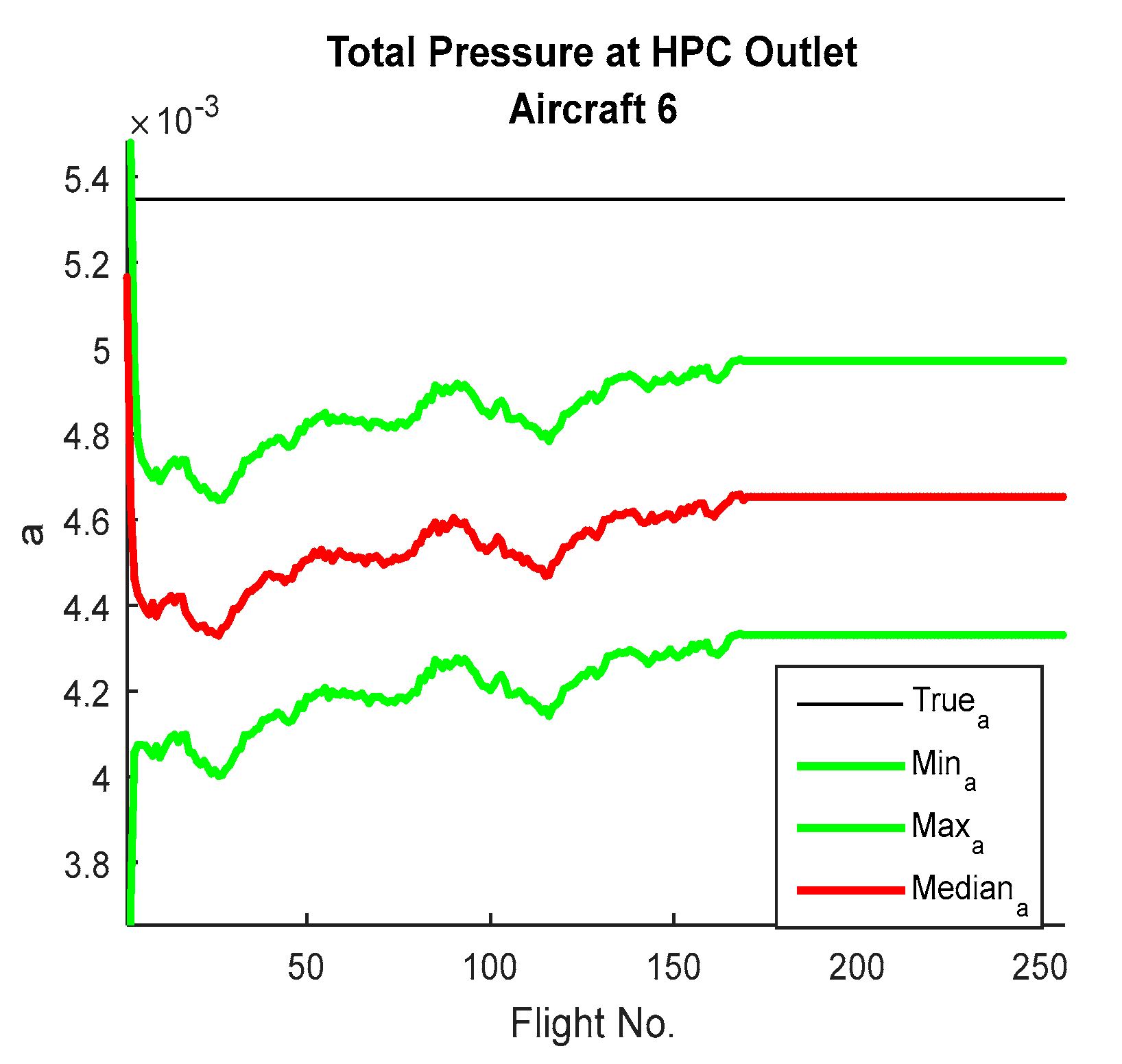
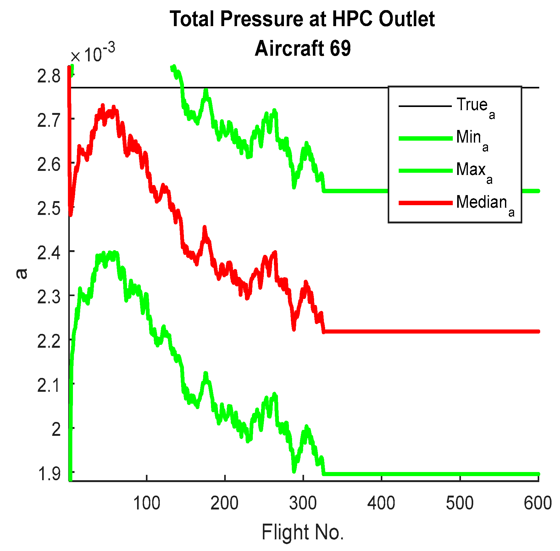
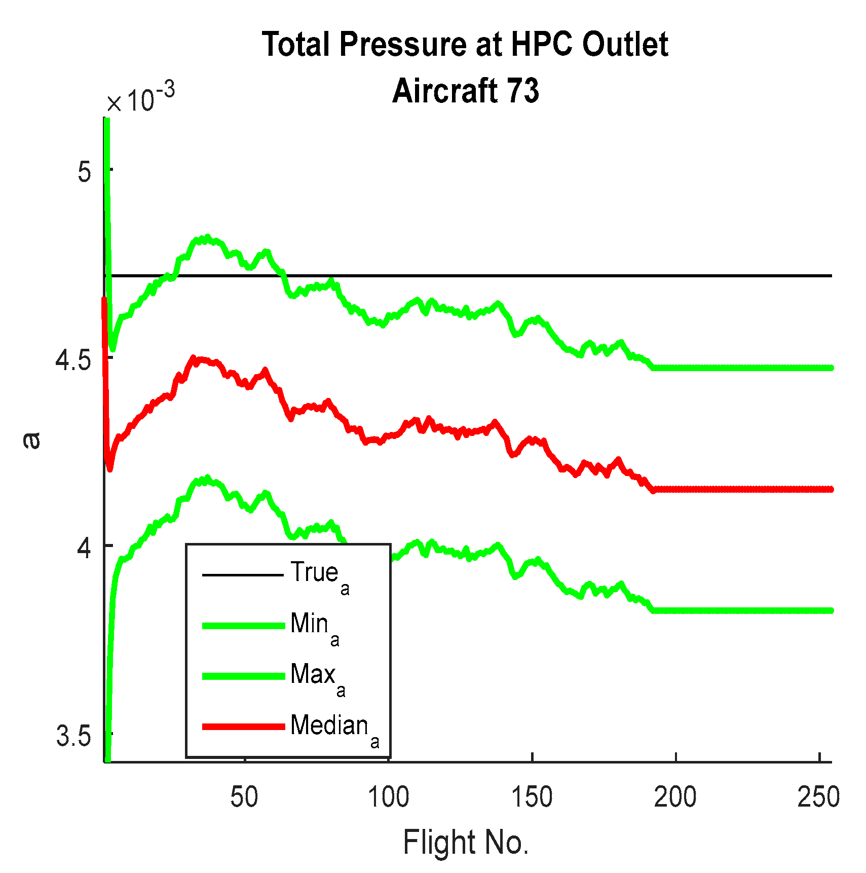
Figure 12, Figure 13, Figure 14 and Figure 15 show the way parameter ‘a’ learned in different engines and how the particle filter is attempting to learn and how it is evaluating over time. Once the value of ‘a’ provides the state estimation which coincides with what has been observed, then it does not have enough errors to be updated dramatically to adapt.
Benchmarking
The Similarity-based Prognostics (SBP) technique has been used to benchmark results. The results have been compared and their adaptability/scalability of the presented technique. The results show that the presented technique has achieved better results in almost all presented cases, results comparison have been demonstrated in the RUL Figure 7, Figure 8, Figure 9 and Figure 10. The presented technique is proven to be an adaptable data-driven technique in comparison the other data-driven methods. The details on the SBP are provided in the next section.
Similarity-Based Prognostics
Similarity-based Prognostics (SBP) is a generic type of prognostic approach where the test specimen signal segments, consisting of sequential raw measurements or processed data are correlated to the previously collected data (i.e., historical data) segments by using a similarity concept. Unlike traditional data-driven models, in SBP, RUL is calculated by aggregating the weighted average of the training sample RUL values rather than extrapolating the test sample’s current health level to a predefined threshold.
Similarity-based Prognostic approach is a simple and powerful algorithm for RUL estimations, notably when the historical training sample size is relatively abundant. In addition, this approach is suitable for the cases where the degradation path is not necessarily exhibiting a monotonic propagation pattern which is difficult to model using parametric approaches [44]. Wang et al. [45] won the Prognostic and Health Management Society’s data challenge competition in 2008 where Wang et al. employed a similarity-based prognostic approach to predict the RUL of turbofan engines created by C-MAPSS simulation.
In similarity-based prognostics, the estimations of RUL involves calculating the similarity between the test sample (i.e., ‘’) and the training samples (i.e., ‘’) as shown in Equation (13). The similarity index is based on the calculated point wise Euclidean distances in between ‘’ sequences of observations. Distance score calculation in between training samples and the test sample at the ‘’ time point formulated in Equation (12). Final RUL estimation of a test sample at a time instance (i.e., ‘’) is achieved by aggregating the weighted average of training samples’ corresponding remaining useful life values as formulated in Equation (14). To be more precise, ‘’ symbolizes the remaining useful life of the ‘’ training sample at ‘’ time point which is obtained by calculating the difference between the training sample’s end-of-life time and the ‘’ time point. The most similar segment to the test segment is specified for each training sample whereas the RUL of the test sample is obtained by taking the weighted average of these training RUL values. In fact, the weights are obtained using the bell-shaped similarity functions.
‘λ’ is an arbitrary parameter which can be set to shape the desired interpretation of similarity, whereas ‘n’ defines the number of latest consecutive observations involved in similarity calculations. The smaller the ‘λ’ is, the stronger the definition of similarity. For instance, a small value for ‘λ’ signifies that the training segment should be very similar to the test segment so that it will be appointed with a similarity value reasonably higher than zero. However, when working with higher decimal point precision systems, this concept becomes trivial as the similarity ratio in between training samples remain the same. Similarity definition parameter ‘λ’ is optimised to enhance the similarity-based prognostic performance. Genetic Algorithm (GA) is employed for optimisation of the parameter [46]. The GA is used rather than trial and error of many lambda values, this reduces the human effort and time for processing. Since prognostic calculation requires extensive amount of data manipulation and it takes time to generate prognostics results. Therefore, it was decided to use GA to optimise the lambda values. The data training sample were 70% and 30% for the testing for SBP and for the presented technique, to provide fair comparison. The 70% and 30% of the data has been selected randomly, to result the algorithm fairly.
The compassion between the presented adaptable data-driven technique to SBP is shown in the Figure 7, Figure 8, Figure 9 and Figure 10 and the error values also has been presented in the Table 2, Table 3, Table 4 and Table 5.
The ratio between the nominal and the adaptable model is more significant if the operating condition of a test sample is more different from the nominal model. Hence this explains the better results as observed in this experiment. Furthermore, SBP technique only provide the results without any lower and upper bounds where the presented technique provides the certainty bounds (lower and upper bounds) and these certainty bounds also be adjusted within the algorithm. Presently these certainty bounds were set on 30% confidence level. The usual censuses in the industry is to keep the certainty bounds to 30%, as the results are precise within those certainty.
7. Concluding Remarks
Vital parts of the integrated health management technology are diagnostics and prognostics. In today’s aircraft the diagnostic and prognostic systems play a crucial part in aircraft safety while reducing the operating and maintenance costs. Prognostics allow anticipation of system failures well ahead of time so that maintenance can be planned, scheduled and performed in the most optimal way.
The expectation of health also enables to minimize the risk of system failure which could lead to catastrophic accidents. Prognostics will be most useful when the component’s operating condition varies from its nominal value and cannot be pre-determined in advance. In most cases, the actual end-of-life of a component can be expected to be significantly different from its manufacturer-defined mean time before failure.
The two most common approaches reported in the literature are data-driven and model-based. The data-driven approach allows complex degradation patterns to be easily captured in the model but has a severe limitation in the operating conditions in which the model is valid. In the model-based approach, a degradation model is explicitly described using mathematical equations with physical meaning. Explicit mathematical representation (often not possible to be derived) allows the relevant model parameters to be scaled online to match a current operating condition. Therefore, a combination of data-driven model and online parameter estimation can be used to address a prognostics problem which has a complex degradation model and large variation in operation conditions, and this is what is proposed in this article.
How fast a system degrades is proportional to its degradation rate which will essentially depend on the operating conditions. If the rate is multiplied by some factors, then this also means we are scaling the time by a proportion of that factor. In order for a data-driven model to be scalable, a scaling parameter will have to be explicitly part of the model. Instead of overall fitting the data, the model (the model presented in this paper) must learn a nominal degradation pattern where different degradation profiles can be fitted by using some appropriate model parameters. This way the data-driven model can be updated to match the current operating conditions, and hence a better prediction because of a more accurate model.
In this case study, it can be seen that the proposed prognostic approach has potential to be applicable in a real-world environment where operating conditions can vary significantly and cannot be accurately defined in advance. The approach can potentially be used in applications where only accelerated testing data are available for the algorithm development. However, its claim as a generic adaptable approach must be further researched in comparison with other engineering examples and with other data-driven techniques, such as Time Delayed Neural Network (TDNN) or similarity-based prognostics (SBP).
Author Contributions
F.K. was the leading researcher for this work, he wrote the article and the presented algorithm was his concept, furthermore he also conducted the whole research work including testing, writing presenting etc. O.E. helped the research work implementation and proof reading, A.K. was provided the engineering, engine aging and physical aspect of this research. W.O. helped in literature review as well as proof reading.
Funding
IVHM Centre and partners has provided the founding of this research study.
Acknowledgments
The authors would like to thank the IVHM (Integrated Vehicle Health Management) Centre and all the partners of the IVHM centre for funding the study and providing the feedback and useful suggestions.
Conflicts of Interest
No conflicts of interest have been found for this research.
References
- Peng, Y.; Wang, Y.; Zi, Y. Switching state-space degradation model with recursive filter/smoother for prognostics of remaining useful life. IEEE Trans. Ind. Inform. 2018. [Google Scholar] [CrossRef]
- Eker, Ö.F.; Camci, F.; Jennions, I.K. Major challenges in prognostics: Study on benchmarking prognostics datasets. In Proceedings of the First European Conference of the Prognostics and Health Management Society, Dresden, Germany, 3–5 July 2012. [Google Scholar]
- Wu, J.; Wu, C.; Cao, S.; Or, W.; Deng, C.; Shao, X. Degradation Data-Driven Time-To-Failure Prognostics Approach for Rolling Element Bearings in Electrical Machines. IEEE Trans. Ind. Electron. 2018, 66, 529–539. [Google Scholar] [CrossRef]
- Zio, E.; Peloni, G. Particle filtering prognostic estimation of the remaining useful life of nonlinear components. Reliabil. Eng. Syst. Saf. 2011, 96, 403–409. [Google Scholar] [CrossRef]
- Heimes, F.O. Recurrent neural networks for remaining useful life estimation. In Proceedings of the International Conference on Prognostics and Health Management, Denver, CO, USA, 6–9 October 2008. [Google Scholar]
- Guo, L.; Li, N.; Jia, F.; Lei, Y.; Lin, J. A recurrent neural network based health indicator for remaining useful life prediction of bearings. Neurocomputing 2017, 240, 98–109. [Google Scholar] [CrossRef]
- Huang, R.; Xi, L.; Li, X.; Liu, C.R.; Qiu, H.; Lee, J. Residual life predictions for ball bearing based on self-organizing map and back propagation neural network methods. Mech. Syst. Signal Process. 2007, 21, 193–207. [Google Scholar] [CrossRef]
- Byington, C.S.; Watson, M.; Edwards, D. Data-driven neural network methodology to remaining life predictions for aircraft actuator components. In Proceedings of the IEEE Aerospace Conference, Big Sky, MT, USA, 6–13 March 2004. [Google Scholar]
- Riad, A.; Elminir, H.; Elattar, H. Evaluation of neural networks in the subject of prognostics as compared to linear regression model. Int. J. Eng. Technol. 2010, 10, 50–56. [Google Scholar]
- Benkedjouh, T.; Medjaher, K.; Zerhouni, N.; Rechak, S. Remaining useful life estimation based on nonlinear feature reduction and support vector regression. Eng. Appl. Artif. Intell. 2013, 26, 1751–1760. [Google Scholar] [CrossRef]
- Khelif, R.; Chebel-Morello, B.; Malinowski, S.; Laajili, E.; Fnaiech, F.; Zerhouni, N. Direct remaining useful life estimation based on support vector regression. IEEE Trans. Ind. Electron. 2017, 64, 2276–2285. [Google Scholar] [CrossRef]
- Medjaher, K.; Tobon-Mejia, D.A.; Zerhouni, N. Remaining useful life estimation of critical components with application to bearing. IEEE Trans. Reliabil. 2012, 61, 292–302. [Google Scholar] [CrossRef] [Green Version]
- Tobon-Mejia, D.A.; Medjaher, K.; Zerhouni, N.; Tripot, G. A data-driven failure prognostics method based on mixture of Gaussions Hidden Markov models. IEEE Trans. Reliabil. 2012, 61, 491–503. [Google Scholar] [CrossRef] [Green Version]
- Liu, D.; Pang, J.; Zhou, J.; Peng, Y.; Pecht, M. Prognostics for state of health estimation of lithium-io batteries based on combination Gaussian process functional regression. Microelectron. Reliabil. 2013, 53, 832–839. [Google Scholar] [CrossRef]
- Liu, Y.; Mohanty, S.; Chattopadhyay, A. A Gaussian Process based prognostics framework for composite structures. In Proceedings of the SPIE, Smart Structures and Materials & Nondestructive, San Diego, CA, USA, 8–12 March 2009. [Google Scholar]
- Si, X.S.; Wang, W.; Hu, C.H.; Zhou, D.H. Remaining useful life estimation—A review on the statistical data driven approaches. Eur. J. Oper. Res. 2011, 213, 1–14. [Google Scholar] [CrossRef]
- Lei, Y.; Li, N.; Guo, L.; Li, N.; Yan, T.; Lin, J. Machinery health prognostics: A systematic review from data acquisition to RUL prediction. Mech. Syst. Signal Process. 2018, 104, 799–834. [Google Scholar] [CrossRef]
- Li, Y.; Billington, S.; Zhang, C.; Kurfess, T.; Danyluk, S.; Liang, S. Adaptive prognostics for rolling element bearing condition. Mech. Syst. Signal Process. 1999, 13, 103–113. [Google Scholar] [CrossRef]
- He, W.; Williard, N.; Osterman, M.; Pecht, M. Prognostics of lithium-ion batteries using extended Kalman filtering. In Proceedings of the IMAPS Advanced Technology Workshop on High Reliability Microelectronics for Military Applications, Linthicum Heights, MD, USA, 17–19 May 2011. [Google Scholar]
- Daigle, M.J.; Goebel, K. Model-based prognostics with concurrent damage progression processes. IEEE Trans. Syst. Man Cybern. 2013, 43, 535–546. [Google Scholar] [CrossRef]
- Daigle, M.; Goebel, K. Model-based prognostics under limited sensing. In Proceedings of the IEEE Aerospace Conference, Big Sky, MT, USA, 6–13 March 2010. [Google Scholar]
- Gorijian, N.; Ma, L.; Mittinty, M.; Yarlagadda, P.; San, Y. A review on degradation models in reliability analysis. In Proceedings of the 4th World Congress on Engineering Asset Management, Athens, Greece, 28–30 September 2009. [Google Scholar]
- Chookah, M.; Nuhi, M.; Modarres, M. A probabilistic physics-of-failure model for prognostic health management of structures subject to pitting and corrosion-fatige. Reliabil. Eng. Syst. Saf. 2011, 96, 1601–1610. [Google Scholar] [CrossRef]
- Tinga, T. Application of physical failure models to enable usage and load based maintenance. Reliabil. Eng. Syst. Saf. 2010, 95, 1061–1075. [Google Scholar] [CrossRef]
- Li, Y.G.; Nilkitsaranont, P. Gas turbine performance prognostic for condition-based maintenance. Appl. Energy 2009, 86, 2152–2161. [Google Scholar] [CrossRef]
- Saxena, A.; Goebel, K.; Simon, D.; Eklund, N. Damage propagation modeling for aircraft engine run-to-failure simulation. In Proceedings of the International Conference on Prognostics and Health Management, Denver, CO, USA, 6–9 October 2008. [Google Scholar]
- Sasahara, O. JT9D engine/module performance deterioration results from back to back testing. In Proceedings of the 7th International Symposium on Air Breathing Engines, Beijing, China, 2–6 September 1985. [Google Scholar]
- Crosby, J. Factors relating to deterioration based on Rolls-Royce RB211 in service performance. Turbomach. Perform. Deterior. 1986, 37, 41–47. [Google Scholar]
- Saxena, A.; Goebel, K. Turbofan Engine Degradation Simulation Data Set, NASA Ames Prognostics Data Repository. Available online: http://ti.arc.nasa.gov/tech/dash/pcoe/prognostic-data-repository/ (accessed on 15 August 2010).
- Wang, C.; Xu, L.; Peng, W. Conceptual design of remote monitoring and fault diagnosis systems. Inf. Syst. 2007, 32, 996–1004. [Google Scholar] [CrossRef]
- Donat, W.; Choi, W.; Singh, S.; Pattipati, K. Data visualization, data reduction and classifier fusion for intelligent fault diagnosis in gas turbine engines. J. Eng. Gas Turb. Power 2008, 130, 041602. [Google Scholar] [CrossRef]
- Bassily, H.; Lund, R.; Wagner, J. Fault detection in multivariate signals with applications to gas turbines. IEEE Trans. Signal Process. 2009, 57, 835–842. [Google Scholar]
- Young, K.; Lee, D.; Vitali, V.; Ming, Y. A fault diagnosis method for industrial gas turbines using Bayesian data analysis. J. Eng. Gas Turb. Power 2010, 132, 041602. [Google Scholar]
- Yu, B.; Liu, D.; Zhang, T. Fault diagnosis for micro-gas turbine engine sensors via wavelet entropy. Sensors 2011, 11, 9928–9941. [Google Scholar] [CrossRef] [PubMed]
- Wu, S.; Wu, P.; Wu, C.; Ding, J.; Wang, C. Bearing fault diagnosis based on multiscale permutation entropy and support vector machine. Entropy 2012, 14, 1343–1356. [Google Scholar] [CrossRef]
- Wu, S.; Wu, C.; Wu, T.; Wang, C. Multi-scale analysis based ball bearing defect diagnostics using Mahalanobis distance and support vector machine. Entropy 2013, 15, 416–433. [Google Scholar] [CrossRef]
- Frederick, D.; De Castro, J.; Litt, J. User’s Guide for the Commercial Modular Acro-Propulsion System Simulation (C-MAPSS); NASA: Cleveland, OH, USA, 2007. [Google Scholar]
- Rios, M.P.; Lopes, H.F. The extended Liu and West filter: Parameter learning in Markov switching stochastic volatility models. In State-Space Models: Applications in Economics and Finance; Springer: New York, NY, USA, 2013; pp. 23–61. [Google Scholar]
- Chen, Z. Bayesian filtering: From Kalman filters to particle filters and beyond. Statistics 2003, 182, 1–69. [Google Scholar] [CrossRef]
- Nemeth, C.; Fearnhead, P.; Mihaylova, L.; Vorley, D. Particle learning methods for state and parameter estimation. In Proceedings of the IET Data Fusion & Target Tracking Conference, London, UK, 16–17 May 2012. [Google Scholar]
- Liu, J.; West, M. Combined parameter and state estimation in simulation-based filtering. In Sequential Monte Carlo Methods in Practice; Springer: New York, NY, USA, 2001; pp. 197–223. [Google Scholar]
- An, D.; Choi, J.H.; Kim, N.H. Prognostics 101: A tutorial for particle filter-based prognostics algorithm using Matlab. Reliabil. Eng. Syst. Saf. 2013, 115, 161–169. [Google Scholar] [CrossRef]
- Saxena, A.; Celaya, J.; Saha, B.; Saha, S.; Goebel, K. Metrics for offline evaluation of prognostic performance. In Proceedings of the Annual Conference of the PHM Society, Portland, OR, USA, 10–14 October 2010. [Google Scholar]
- Wang, T. Trajectory Similarity Based Prediction for Remaining Useful Life Estimation. Ph.D. Thesis, University of Cincinnati, Cincinnati, OH, USA, 2010. [Google Scholar]
- Wang, T.; Yu, J.; Siegel, D.; Lee, J. A similarity-based prognostics approach for Remaining Useful Life estimation of engineered systems. In Proceedings of the International Conference on Prognostics and Health Management, Denver, CO, USA, 6–9 October 2008. [Google Scholar]
- Zio, E.; Di Maio, F. A data-driven fuzzy approach for predicting the remaining useful life in dynamic failure scenarios of a nuclear system. Reliabil. Eng. Syst. Saf. 2010, 95, 49–57. [Google Scholar] [CrossRef] [Green Version]
Figure 1.
Prognostic and diagnostic phases in Condition Based & Predictive Maintenance [2].
Figure 1.
Prognostic and diagnostic phases in Condition Based & Predictive Maintenance [2].

Figure 2.
Gas turbine Engine dataset architecture [29]. (a) Simplified diagram for the aircraft gas turbine engine, (b) A layout of modules and connections in the simulation.
Figure 2.
Gas turbine Engine dataset architecture [29]. (a) Simplified diagram for the aircraft gas turbine engine, (b) A layout of modules and connections in the simulation.

Figure 3.
Initial HI (Health Index) for Component.

Figure 4.
Degradation of the of health index of component/sub-system.

Figure 5.
Radial Network Measurement Function.


Figure 7.
RUL Calculation of 4 Selection Sensors for Engine 73.

Figure 8.
RUL Calculation of 4 Selection Sensors for Engine 39.

Figure 9.
RUL Calculation of 4 Selection Sensors for Engine 69.

Figure 10.
RUL Calculation of 4 Selection Sensors for Engine 73.

Figure 11.
The Neural Network results of 14 sensors of Turbofan Jet Engine.

Figure 12.
Parameter ‘a’ learning for Engine 6 sensor Total Pressure at HPC Outlet.

Figure 13.
Parameter ‘a’ learning for Engine 39 sensor Total Pressure at HPC Outlet.

Figure 14.
Parameter ‘a’ learning for Engine 69 sensor Total Pressure at HPC Outlet.

Figure 15.
Parameter ‘a’ learning for Engine 73 sensor Total Pressure at HPC Outlet.


Table 1.
Description of the Sensor Signals for the Aircraft Gas Turbine Engine Dataset [29].
Table 1.
Description of the Sensor Signals for the Aircraft Gas Turbine Engine Dataset [29].
| Index | Symbol | Description | Units |
|---|---|---|---|
| 1 | T2 | Total Temperature at fan inlet | °R |
| 2 | T24 | Total temperature at LPC outlet | °R |
| 3 | T30 | Total temperature at HPC outlet | °R |
| 4 | T50 | Total temperature LPT outlet | °R |
| 5 | P2 | Pressure at fan inlet | psia |
| 6 | P15 | Total pressure in bypass-duct | psia |
| 7 | P30 | Total pressure at HPC outlet | psia |
| 8 | Nf | Physical fan speed | rpm |
| 9 | Nc | Physical core speed | rpm |
| 10 | Epr | Engine pressure ratio | -- |
| 11 | Ps30 | Static pressure at HPC outlet | psia |
| 12 | Phi | Ratio of fuel flow to Ps30 | psi |
| 13 | NRf | Corrected fan speed | rpm |
| 14 | NRc | Corrected core speed | rpm |
| 15 | BPR | Bypass ratio | -- |
| 16 | farB | Burner fuel-air ratio | -- |
| 17 | htBleed | Bleed enthalpy | -- |
| 18 | Nf_dmd | Demanded fan speed | rpm |
| 19 | PCNfR_dmd | Demanded corrected fan speed | rpm |
| 20 | W31 | HPT coolant bleed | lbm/s |
| 21 | W32 | LPT coolant bleed | lbm/s |
°R: The Rankine temperature scale; psia: Pounds per square inch absolute; rpm: Revolution per minute; pps: Pulse per second; psi: Pounds per square inch; lbm/s: Pound mass per second.
Table 2.
Remaining Useful Life () Prediction Error for Sensor Static Pressure at HPC Outlet.
| Data-Driven Techniques and Models | Root-Mean-Square-Error (RMSE) and Mean Absolute Percent Error (MAPE) | ||||
|---|---|---|---|---|---|
| Engine 6 | Engine 39 | Engine 69 | Engine 73 | Error Calculation Method | |
| RBF NN + PF | 12.12 | 9.30 | 68.91 | 24.80 | RMSE |
| 19.53 | 19.65 | 86.32 | 25.87 | MAPE (%) | |
| SBP | 31.04 | 24.21 | 88.04 | 49.95 | RMSE |
| 36.15 | 50.81 | 38.78 | 45.18 | MAPE (%) | |
 RBF NN +PF;
  SBP.
SBP.Table 3.
Remaining Useful Life () Prediction Error for Sensor Total Pressure HPC Outlet.
| Data-Driven Techniques and Models | Root-Mean-Square-Error (RMSE) and Mean Absolute Percent Error (MAPE) | ||||
|---|---|---|---|---|---|
| Engine 6 | Engine 39 | Engine 69 | Engine 73 | Error Calculation Method | |
| RBF NN + PF | 10.78 | 5.17 | 72.78 | 19.04 | RMSE |
| 18.43 | 15.78 | 104.89 | 18.85 | MAPE (%) | |
| SBP | 36.86 | 31.86 | 86.25 | 53.07 | RMSE |
| 36.62 | 69.46 | 37.22 | 46.22 | MAPE (%) | |
RBF NN +PF; SBP.Table 4.
Remaining Useful Life () Prediction Error for Sensor Ratio of fuel flow to Ps30.
| Data-Driven Techniques and Models | Root-Mean-Square-Error (RMSE) and Mean Absolute Percent Error (MAPE) | ||||
|---|---|---|---|---|---|
| Engine 6 | Engine 39 | Engine 69 | Engine 73 | Error Calculation Method | |
| RBF NN + PF | 11.57 | 8.43 | 63.35 | 19.04 | RMSE |
| 16.32 | 25.69 | 81.42 | 23.59 | MAPE (%) | |
| SBP | 31.86 | 22.49 | 84.08 | 55.76 | RMSE |
| 36.48 | 49.71 | 40.67 | 49.73 | MAPE (%) | |
RBF NN +PF; SBP.Table 5.
Remaining Useful Life () Prediction Error for Sensor LPT coolant bleed.
| Data-Driven Techniques and Models | Root-Mean-Square-Error (RMSE) and Mean Absolute Percent Error (MAPE) | ||||
|---|---|---|---|---|---|
| Engine 6 | Engine 39 | Engine 69 | Engine 73 | Error Calculation Method | |
| RBF NN + PF | 12.91 | 3.59 | 95.75 | 14.76 | RMSE |
| 35.44 | 13.39 | 124.24 | 30.03 | MAPE (%) | |
| SBP | 30.81 | 44.17 | 81.10 | 40.9 | RMSE |
| 40.82 | 104.76 | 39.30 | 41.00 | MAPE (%) | |
RBF NN +PF; SBP.© 2018 by the authors. Licensee MDPI, Basel, Switzerland. This article is an open access article distributed under the terms and conditions of the Creative Commons Attribution (CC BY) license (http://creativecommons.org/licenses/by/4.0/).
Share and Cite
MDPI and ACS Style
Khan, F.; Eker, O.F.; Khan, A.; Orfali, W. Adaptive Degradation Prognostic Reasoning by Particle Filter with a Neural Network Degradation Model for Turbofan Jet Engine. Data 2018, 3, 49. https://doi.org/10.3390/data3040049
AMA Style
Khan F, Eker OF, Khan A, Orfali W. Adaptive Degradation Prognostic Reasoning by Particle Filter with a Neural Network Degradation Model for Turbofan Jet Engine. Data. 2018; 3(4):49. https://doi.org/10.3390/data3040049
Chicago/Turabian StyleKhan, Faisal, Omer F. Eker, Atif Khan, and Wasim Orfali. 2018. "Adaptive Degradation Prognostic Reasoning by Particle Filter with a Neural Network Degradation Model for Turbofan Jet Engine" Data 3, no. 4: 49. https://doi.org/10.3390/data3040049