Basic Features of the Analysis of Germination Data with Generalized Linear Mixed Models


Council for Agricultural Research and Economics—Research Centre for Genomics and Bioinformatics, via S. Protaso 302, 29017 Fiorenzuola d’Arda (PC), Italy
Data 2020, 5(1), 6; https://doi.org/10.3390/data5010006
Submission received: 29 November 2019
/
Accepted: 4 January 2020
/
Published: 8 January 2020
Abstract
:Germination data are discrete and binomial. Although analysis of variance (ANOVA) has long been used for the statistical analysis of these data, generalized linear mixed models (GzLMMs) provide a more consistent theoretical framework. GzLMMs are suitable for final germination percentages (FGP) as well as longitudinal studies of germination time-courses. Germination indices (i.e., single-value parameters summarizing the results of a germination assay by combining the level and rapidity of germination) and other data with a Gaussian error distribution can be analyzed too. There are, however, different kinds of GzLMMs: Conditional (i.e., random effects are modeled as deviations from the general intercept with a specific covariance structure), marginal (i.e., random effects are modeled solely as a variance/covariance structure of the error terms), and quasi-marginal (some random effects are modeled as deviations from the intercept and some are modeled as a covariance structure of the error terms) models can be applied to the same data. It is shown that: (a) For germination data, conditional, marginal, and quasi-marginal GzLMMs tend to converge to a similar inference; (b) conditional models are the first choice for FGP; (c) marginal or quasi-marginal models are more suited for longitudinal studies, although conditional models lead to a congruent inference; (d) in general, common random factors are better dealt with as random intercepts, whereas serial correlation is easier to model in terms of the covariance structure of the error terms; (e) germination indices are not binomial and can be easier to analyze with a marginal model; (f) in boundary conditions (when some means approach 0% or 100%), conditional models with an integral approximation of true likelihood are more appropriate; in non-boundary conditions, (g) germination data can be fitted with default pseudo-likelihood estimation techniques, on the basis of the SAS-based code templates provided here; (h) GzLMMs are remarkably good for the analysis of germination data except if some means are 0% or 100%. In this case, alternative statistical approaches may be used, such as survival analysis or linear mixed models (LMMs) with transformed data, unless an ad hoc data adjustment in estimates of limit means is considered, either experimentally or computationally. This review is intended as a basic tutorial for the application of GzLMMs, and is, therefore, of interest primarily to researchers in the agricultural sciences.
1. Introduction
For plants, germination is a developmental process that commences with the uptake of water by the quiescent dry seed (except for unorthodox seeds) and terminates with the piercing of the seed coat owing to the start of elongation of the embryonic axis [1,2].
Germination studies can be either controlled experiments, i.e., germination tests, or observational studies, chiefly in the field of ecology. Both furnish data that can be analyzed according to a statistical model (see [3] for a non-trivial illustration of what a statistical model is). However, whereas controlled experiments have a well-defined design aiming at establishing the effect of some pre-selected factors whose levels are controlled by the researcher [4], observational studies strive to find out the most important factors affecting germination in a complex, uncontrolled environment [5]. Typically, biometric or other seed-specific traits and several environmental variables are simultaneously recorded and evaluated in the latter case. Hence, observational studies easily incur collinearity of predictors [5,6], while germination tests do not (though some variance/covariance structures may be responsible for similar troubles). Accordingly, model selection, as regards the choice of factors to be included into the model, is a pre-eminent target of observational studies, but not of germination tests. Nonetheless, even data from germination tests can be analyzed with diverse models, but the main differences among these models are related to the statistical theory, rather than to the selection of ecological, or biological, factors. The present paper focuses on the analysis of germination data with generalized linear mixed models (GzLMMs) and concerns the application of such models to germination tests, for which some examples that are representative of common experimental setups are provided. Observational studies are more variable in their experimental designs than germination tests and are not considered here. Notwithstanding this caveat, many basic features of GzLMMs highlighted here also apply to observational studies. It is worth noticing that the acronym GzLMM is used in this review even though the literature seems to have converged on GLMM [3]. The reason for this choice is that some readers could be confused by the previous use of GLM (as with the homonym SAS procedure), which stood for ‘general linear model’. In the recent literature, this kind of models are usually addressed as linear models (LMs), by dropping the ‘General’ specification, so that ‘G’, rather than ‘Gz’ is now used to indicate ‘generalized’ [3]. As GzLMMs are a kind of linear models, it was preferred to use ‘LMs’ to indicate the whole family of linear models, and to keep the old-fashioned ‘GLMs’ when referring to “General linear models”.
Experiments always confront the variability that emerges at various levels of data collection and any finding is, therefore, subject to probabilistic interpretation [5,7]. This is typically dealt with by applying statistics. Classical approaches in the statistical analysis of germination data have been critiqued [8], and GzLMMs have been proposed to solve most criticisms [9].
In this review, the basic aspects of GzLMMs are presented and discussed focusing on germination data. Some datasets from germination tests are analyzed with GzLMMs by using SAS Studio software, comparing different methodological approaches for the statistical analysis of this kind of data. Detailed comments and software tips are placed in Annexes supplementary to the main text. The objective of this review is to provide a basic tutorial explaining the use of GzLMMs for the benefit of researchers in the agricultural field who are not familiar with this statistical method. To this end, I collected in a single paper all the information necessary to understand the basic features of the GzLMMs and that is currently scattered across multiple sources.
1.1. Germination Tests
Germination is routinely tested by taking small representative random samples of seeds from a seed lot and examining their responses under standard conditions or in the presence of selected factors, and data collected on such small samples can then be used to infer the quality of the entire lot, or its general response, following the application of appropriate statistical methods [7,8].
If the conditions are optimal, i.e., such that most seeds germinate, and/or are representative of typical field conditions, the test is typically aimed at estimating the germination capability of the seed lot (as assessed within a suitable time after which there is little additional germination). For agronomic purposes, the number of seeds producing healthy sprouts is usually recorded because, in this case, the intent of germination tests is to be predictive of the number of seeds that can establish a healthy seedling in the field, that is, two different accomplishments are taken into account: Germination and healthiness.
In physiological studies, the number of seeds that attain visible germination is considered, since germination and healthiness are distinct phenomena and have, therefore, to be analyzed separately. In this respect, seed dormancy, i.e., the failure of an intact viable seed to complete germination under favorable conditions can be measured in terms of reduced germination [2,10], provided that a suitable control is made for distinguishing the proportion of seeds that do not germinate because are dormant from the proportion of seeds that do not germinate because are dead. Testing germination under suboptimal conditions, or after some treatment, provides important indications about the response of germination, or dormancy, to the studied conditions/treatment.
Agronomical and physiological studies also differ in other ways. Whereas the former kind of experiments may admit truncation of observations after some convenient time of germination, physiological studies typically should not be too restrictive, as the last germinating seeds represent an informative component of the seed population. Recording germination must end after some suitable time not only because of practical reasons but also because different processes can ultimately supersede germination [11,12]. Choosing a proper test duration for the studied species is a very important part of the experimental design.
All these aspects characterizing a germination test must be defined before any statistical analysis is performed.
1.2. Germination Data
Germination tests provide categorical (nominal) dichotomous data (i.e., yes/no germination of each seed) for a dependent (response) variable, i.e., germination. These data are dichotomous as there can only be one of two possible outcomes, generically referred to as success/failure events, in a process denoted as Bernoulli trial. Germination can be assessed across time or for a single testing time (usually, at the end of the test, that is, the final germination percentage, FGP, is recorded). In the former case, either germination curves, which record the progress of germination through time under given testing conditions, or after-ripening curves, corresponding to changes of dormancy with increasing times of dry warm storage, are obtained.
Germination data can be arranged either as binary data (individual Bernoulli outcomes, with every response being either an event or a nonevent), that is, the response of every individual seed is kept as a separate record (commonly, a line in the dataset), or, more frequently, data can be arranged as means of binomial proportions across clusters, that is, means of aggregate binary responses. Clustered data arise when multiple observations are collected on the same sampling or experimental unit, e.g., Petri dishes, within which seeds are aggregated. Different statistical approaches are best suited to the two arrangements of data. Individual seed responses are considered when time-to-event, aka survival, analysis is used to compare germination time-courses [13,14], whereas the fraction of germinated seeds in each Petri dish, or plate, is recorded when a method based on the analysis of variance is used [4,9]. In the latter case, germination data can be expressed either as proportions of germinating seeds with respect to tested seeds (values from 0 to 1), or as percentages (%, i.e., proportions times 100). In any case, germination data follow a binomial distribution, which is characterized by being bounded between a low (0, or 0%) and a high (1, or 100%) limit, and by corresponding to discrete proportions, that is, they are based on counts of a defined number (n) of Bernoulli trials that consist of positive integers between 0 and n, where n is the number of observational units (seeds) that are under trial [4,15,16].
Notice that, differently from count-based discrete proportions, continuous proportions, like the percentage area affected by some perturbation, have a Beta distribution rather than a binomial one [3]. Also, note that binomial counts are records of Y events out of n trials, where n is predetermined by the researcher, whereas counts of events not limited by a predefined upper limit (i.e., when n is not preestablished) follow a Poisson or a negative binomial distribution [7,16].
1.3. The Binomial Distribution
The binomial distribution is a distribution of sample frequencies. Given some fixed conditions, the binomial probability that a discrete observation drawn at random has the characteristic of interest (Y; here, germination) out of a dichotomous alternative (here, a seed does or does not germinate), is the theoretical, unknown in ordinary experiments, pi value, where i defines a specific combination of determining factors. For a single observation, pi is the theoretical probability of a Bernoulli event; when, instead, an aggregate sample of two or more observations is considered, a distribution of possible combinatorial outcomes, having different probabilities, can be predicted based on pi, and such distribution is called binomial. It is implicit in discussing the binomial probability, pi, that every observational unit (i.e., the Bernoulli trial; here, a tested seed) is fated to either one or the other Bernoulli outcome (i.e., to germinate or not to germinate) under investigation (independently of whether we can preventively know the individual fates of the seeds), and that pi (the probability of germination) is a characteristic of the specific (seed) population examined under the given conditions.
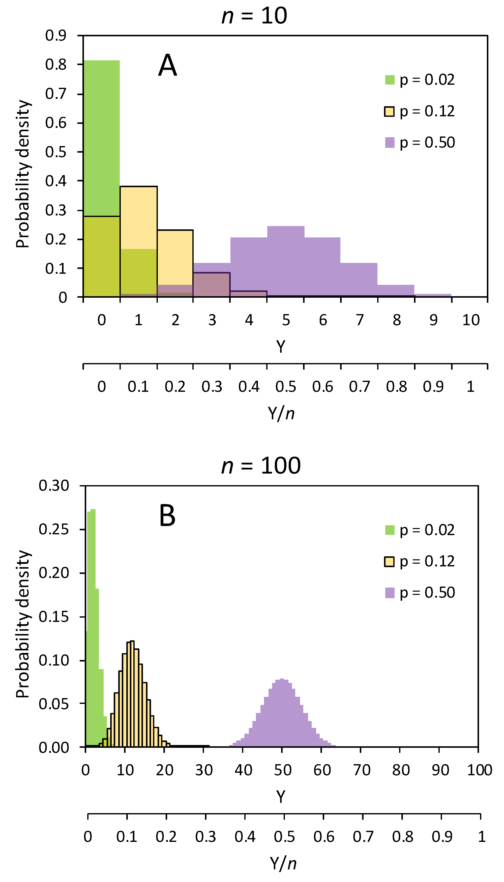
Notice that, whilst the Gaussian distribution is a distribution of values of individuals, the binomial distribution is a distribution of samples of individuals (where individuals are observational units). In other words, whereas the Gaussian distribution is a probability distribution of quantitative effects among a population of observational units, the binomial distribution is a probability distribution of sampling estimates of the discrete number of successful events (Y) for an infinite population of samples, each of n observational units (in such case, the theoretical expected frequencies of the various sampling outcomes are called probability densities). As n is pre-fixed, the distribution of pi estimates (proportions, or percentages) based on the Y/n ratio is often reported in place of Y, as the former represents a normalized binomial distribution (Figure 1). Thus, a binomial distribution with parameters n and pi is the discrete probability distribution of frequencies (counts, proportions, or percentages) of success (i.e., the occurrence of the event under investigation) across infinite independent samplings, each consisting of n Bernoulli trials (i.e., observational units examined for a Bernoulli outcome).
In terms of counts, and for a given n, the expected value of the binomial random variable is npi [15], which, in practice, corresponds to the expected mean number of events when more than one Bernoulli trial is examined (that is, more than one seed is observed). The observed binomial response variable is Y, the number of germinated seeds, which, given n, is used to compute the discrete sample proportion Y/n, i.e., the observed events/trials ratio (here, the ratio of germinated/tested seeds; which is discrete because seeds are discrete entities), which is utilized to estimate pi [15].
The variance of a binomial distribution is the variance among random samples solely due to the theoretical random deviations from pi occurring, during the sampling process, in the assortment of observational units fated to one or the other outcome. It is inherently heteroskedastic (Figure 1), varying, in terms of counts, depending on the mean as npi(1 − pi) [15]. As the larger n is, the higher the number of possible discrete assortments becomes, the variance of the binomial distribution (for a given pi) appears to increase with n when is represented using counts on the x-axis (compare the count scale, Y, of plots A and B in Figure 1). The modal assortment(s) will be npi, or the assortment(s) closest to it if npi is not an integer, and the next adjacent assortments correspond to subsequent Y changes of one unit down to zero counts on one side and up to n counts on the other. So, the higher n is, the wider the counts distribution extends before reaching its extreme limits. The binomial distribution of counts has, therefore, no fixed upper boundary, although it is restrained to be between 0 and n.
In terms of proportions, rather than of counts, the expected value of the discrete random variable is simply pi, which is the probability toward which the observed Y/n ratio is expected to converge for increasing n. In contrast to the binomial distribution of counts, the binomial distribution of discrete proportions is bounded between 0 and 1 on a probabilistic scale, as it is normalized to n (Figure 1). If the theoretical seed population were perfectly uniform, the whole seed lot would either germinate or not germinate; thus, any seed sample would have a Y/n germination ratio of either 0 or 1 [15]. No variability of the germination response would occur among seeds, and the sampling variance would be null. On the other hand, any value of pi between 0 and 1 is associated with some variability in the dichotomous germination response among seeds, and such variation reflects in a sampling variance established according to pi (at a specific combination of experimental factors). Thus, the closer the mean response is to either scale boundary (0 or 1), the more the variance tends to decrease, and skewness tends to increase (Figure 1) [9,15]. The theoretical between-samples binomial variance of the observed Y/n ratio (which is the estimator of the population proportion pi) is pi(1 − pi)/n [15]; that is, the sampling variance of the estimates of pi among plates (i.e., Petri dishes within which seeds are clustered) is smaller for larger values of n. In fact, as variances are quadratic functions of the dependent variable, the binomial variance of the proportion is linked to the binomial variance of counts by the relationship: var(Y/n) = [var(Y)]/n2. Hence, as n increases, the distribution of proportions becomes increasingly narrower around its mean [17], and, of course, increasingly higher in terms of frequencies (which, for a theoretical infinite population, become probability densities), since its overall area, or, better, the sum of all the possible outcoming discrete sampling frequencies, amounts to 1 (Figure 1).
Whilst the binomial distribution of counts might be computationally likened to a Gaussian distribution of individual values (and, thus, the square root of its variance is the standard deviation), the binomial distribution of proportions is equivalent to a distribution of means (since the Y/n of each sample provides an estimate of the population’s pi). Hence, the binomial variance of pi essentially represents a variance of means [15]; although, more exactly, it is a variance of pi estimates for samples of n Bernoulli trials. It, therefore, corresponds to the sampling variance of means for a Gaussian distribution [15]. In this sense, pi is considered the mean (probability), or expectation, of the binomial distribution of proportions, although it is a probability rather than a mean trait value.
As in the Gaussian distribution, the standard error of the mean pi estimate is the square root of the sampling variance (of the pi estimates), that is, . As variances have squared units, the square root transformation is typically necessary to obtain a measure of variability on the scale of the means. Hence, the observed Y/n is expected to become a better estimator of pi, the germination probability of the theoretical seed population, as n increases to infinity, because the standard error of the pi estimates shrinks with inverse relation to . Correspondingly, the number of seeds per Petri dish is the most influential factor affecting the bias and precision of estimates [18].
1.4. The Gaussian Approximation
As the binomial variance, either in terms of counts or proportions, is theoretically determined once the mean, npi or pi, respectively, has been estimated, an interesting feature of binomial data is, therefore, that plate replication is not really necessary to establish the sampling error. Nonetheless, the presence of plates allows a better experimental control of accidental effects, as well as of any heterogeneity of the seed sample or of the treatment. In fact, even though the observational unit for germination data is the individual seed, it is important to note that tests are typically conducted by grouping the seeds into plates (or other suitable containers) so that they can be managed more easily. Thereby, plates also provide a better experimental control (confinement) against accidental factors (like molds) that can affect (kill) the seeds and, thus, interfere with the experimental results. A heavily infected plate can be entirely discharged if this—or another unforeseen setback that invalidates the analysis—can be properly identified and delimited. In this respect, grouping the seeds into plates allows the statistical control of unidentified, accidental factors that can increase the observed variability of the data. Plates are, therefore, experimental units, that is, the smallest units providing random variation and to which randomization should then be applied [3,9,19]. Thus, they are also called units of replication, that is, the smallest entities that are independently assigned a factor level [3]. Clustering seeds in plates also help detecting seed heterogeneity, as it will be discussed.
Using plates is, thus, a common feature of the experimental design of germination tests, and this has, of course, a statistical interpretation. Having a Y/n ratio for every plate, the population pi is estimated as the mean Y/n across plates. If n is constant across plates, this actually consists of using the sum of all the counts across plates (with the same combination of treatment levels) and the sum of all the seeds across these plates to obtain an overall estimation of pi. This overall Y/n ratio is, of course, a better estimator of pi than ratios from individual plates are. As plates are (theoretically independent) samples of size n drawn from a seed population whose binomial response is centered on germination probability pi, the variance among plates is expected to provide an estimate of pi (1 – pi)/n. Although the binomial distribution does not admit a direct estimation of the sampling variance, which is instead calculated from the estimate of pi, it is nonetheless possible to approximate the binomial distribution of pi estimates with a Gaussian distribution, which allows a direct estimation of the variance, independently of the pi estimate. If n is large enough, and pi is not too close to 0 or 1, the binomial distribution indeed appears quite symmetric (Figure 1). In fact, the Central Limit Theorem states that as the number of random samples taken from a population of values of a random variable—even a discrete one—increases, the mean of all samples converges toward the mean of the population, and the sampling distribution of the means of those independent samples will become approximately Gaussian [20].
Even though the variance among plates is expected to be the theoretical binomial variance pi (1 − pi)/n, the observed between-plates variance is, therefore, typically calculated with the normal variance formula , where N is the number of plates. In this way, we have two different calculations of the sampling variance: A binomial one, theoretically computed from the overall, across plates, estimate of pi, and a Gaussian one, based on the observed between-plates variance. They might seem redundant, but, of course, these two variances actually converge only if plates correspond to no other effect than the variability consequent to the random assortment due to sampling. This implies that all the seeds indeed belong to the same population, characterized by germination probability pi. In this respect, it might be worth remarking that values of pi diverse from 0 and 1 reveal an inherent random variability among the population members. In fact, the between-plates variance component due to the binomial sampling variance exists because of the random variability existing among seeds, which, for populations with pi diverse from 0 and 1, translates into a dichotomous germination response [21]. This is, anyway, an essential feature of a population, as it depends uniquely on the population’s pi, so that such inherent seed variability is what causes a binomial variance to be different from zero.
If, however, the seeds do not all belong to the same population characterized by a specific value of the germination probability pi, and/or if plates differ for some effect additional to the random assortment during sampling, the actual variability can only be evaluated as Gaussian variance among plates. The observed variability is then expected to include an additional variance component, in excess of pi(1 − pi)/n, due to the heterogeneity between mixed seed populations [7] and/or among plates (including a non-uniform treatment application). Any additional between-plates variance component is itself a random effect. For a large n, the distribution of such effect ought to be approximately Gaussian, since random effects are assumed to be centered on the mean and sum up to zero, so that they should be roughly symmetric, at least for means not close to 0 or 1.
Noticeably, using a Gaussian approximation to calculate the between-plates variance implies a sort of conceptual shift that justifies the change of the formula and of the underpinning probability distribution used to compute the variance. In fact, the binomial variance corresponds to a discrete distribution of (probabilities/frequencies of) samples, whereas the Gaussian variance represents a distribution of some continuous trait of individuals. To make this clearer, the individuals (observational units) are seeds for the binomial distribution but plates for the Gaussian approximation. This is, of course, an approximation indeed, because the seeds are always to be individually checked, and they are, therefore, the true observational units in any case. As mentioned above, the reason for resorting to this shift is that the Gaussian approximation can account for additional variance components of the variance among plates, whereas the binomial variance cannot. As said, whilst the Gaussian variance of the observed Y/n ratio is expected to estimate the theoretical binomial sampling variance in the absence of other variance components, any additional variance component can be detected by comparing the observed Gaussian between-plates variance with the theoretical binomial variance inferred from the estimate of pi. The presence of additional variance with respect to the binomial one represents what is called over-dispersion (i.e., the ratio between the observed Gaussian variance and the estimated binomial variance), an important parameter for GzLMMs [22].
Although for large values of n the binomial distribution approximates the Gaussian, especially when pi = 0.5 (Figure 1), there is no general agreement about what, in practice, qualifies as “large” [9]. This usually depends on the precision required for the analysis. In germination tests, a minimal requirement for the approximation to be reliable is that npi ≥ 5 for pi < 0.5, and n(1 − pi) ≥ 5 for pi > 0.5 [9]. Thence, indicatively, the approximation may become acceptable even for pi = 0.05 (i.e., 5% germination) and pi = 0.95 (i.e., 95% germination) if there are at least 100 seeds per plate [3]. On the one hand, this means that increasing the number of seeds per plate is the most effective approach to approximating a Gaussian error distribution. With a low number of seeds per plate, a poor approximation is usually obtained.
On the other hand, the larger the number of binomial samples, i.e., plates, the better the Gaussian variance of the observed Y/n ratio is expected to estimate the real between-samples variance, inclusive of pi(1 − pi)/n plus any other between-plates variance component. Thus, as the number of plates increases, over-dispersion can be measured with greater precision. Altogether, greater precision of inference is achieved when both the number of plates and of seeds per plate is large. Specifically, on the one hand, given n, a larger number of plates (N) improves the estimation of pi as well as of the between-plates variance, and, thus, of over-dispersion. On the other hand, given N, a larger number of seeds per plate (n) reduces the sampling variance and thereby increases the precision of the estimate of pi [20]. In practice, greater statistical power can be obtained by allocating seeds so as to have at least 5–6 replicate plates with at least 20–25 seeds per plate rather than fewer plates with more seeds per plate [8]. It is also sensible never to use more than 50–100 seeds per plate, which are enough to provide a reasonable to good Gaussian approximation, respectively (unless pi is very close to 0 or 1), and rather increase the number of plates when possible. In this respect, long ago it was suggested that when the number of seeds under analysis exceeds 400, the asymmetry in the distribution may be usually disregarded, and the Gaussian approximation applies satisfactorily [23]. In fact, four replicates of 100 seeds are recommended by the International Seed Testing Association (ISTA) for standard germination tests. Although fewer seeds may be tested, there should not be fewer than 100 seeds in replicates of 25 or 50 seeds [24].
As explained, plates are random samples of seeds, and therefore, the plate effect can be considered a random factor, that is, plates are clusters of seeds whose aggregate responses represent random deviations from the expectation of pi for every specific combination of determining (fixed) factors. Random factors are typically modeled as deviations from the intercept [22]. In general, the interaction (or nesting) term based on a random factor is used to test the significance of the fixed factor hierarchically above it in the experimental design, and therefore, there should be enough levels of the random factor so that the variance of the interaction, or nesting, term can be estimated with reasonable precision and can have enough degrees of freedom to make the test of the fixed effect reasonably powerful [5]. The trustworthiness and exactness of the inference based on these tests may thus also depend on the number of levels of the random factor, i.e., on how many plates we use [5]. Using too few seeds per plate reduces the accuracy and precision of standard errors [18,20].
1.5. Classical ANOVA
The statistical analysis of germination data is frequently performed by using classical analysis of variance (ANOVA) models and comparison of means tests on the basis of replicated plates [8]. In germination tests, plates might also be considered as blocks, since they correspond to random effects that can account for some unmodeled experimental variability (but we will see that this likening is inappropriate). In addition, by the Central Limit Theorem, plate replication provides a statistical evaluation of the standard errors of the germination means, which are, therefore, more suited to ANOVA and comparison of means tests just because they (the means of the replicate plates) tend to approximate a normal distribution of the errors. Thus, plates are usually considered sampling (or experimental) units.
Unfortunately, two basic assumptions of ANOVA and ANOVA-related comparison of means tests are that residuals are distributed normally around the modeled means and that their variances are homogeneous (near-normality and homoskedasticity of the residuals are essential for p-values computed from the F distribution to be meaningful); both assumptions are often violated by germination data, sometimes severely [8]. Additionally, the chief problem of analyzing germination data with classical approaches based on a Gaussian error distribution (namely, ANOVA and related separation of means tests), i.e., heterogeneity of variances, cannot be amended by any application of the Central Limit Theorem. Nonetheless, if these assumptions approximately hold, a binomial distribution can be reasonably approximated to a normal distribution [15,17]. The approximation is reasonable at half way between the two limits (that is, at 0.5, or 50%), where it is symmetrical, whereas it tends to an asymmetrical distribution as the data approximate the limits, with increasing right skewedness when approaching the lower limit (where the errors approximate a Poisson distribution) or left skewedness toward the upper limit. Indeed, the binomial distribution converges toward the Poisson distribution as the number of trials goes to infinity and pi tends toward zero [7].
As a rule of thumb, data in the 30%–70% range (i.e., 0.3–0.7 range of proportions) may be analyzed even for relatively small experiments because classical ANOVA is robust to small violations of normality [17], and though it is more sensitive to violations of the assumption of equal variances, when the groups (i.e., the various combinations of the levels of the fixed factors) are all about the same size, ANOVA is still relatively robust unless the group variances are extremely different [15]. Wide differences are not the case for purely binomial data in the 0.3–0.7 range of proportions.
To apply ANOVA to data outside the above-mentioned range, a common solution is to perform an angular transformation of the data [15], which “stretches” the range of the binomial data with greater effect as they are close to the 0–1 boundaries [17], thereby increasing the variances at the two tails more than happens for data closer to 0.5 (50%). In fact, the angular transformation stabilizes the variance of binomial data, in the sense that it becomes approximately constant after transformation if the data are balanced [25]. In this way, the natural binomial heteroskedasticity (with lower variance toward the boundaries) as well as the non-normality (skewedness) are somewhat counterbalanced [15].
The angular transformation is typically preferred for binomial data because it is quite symmetrical across the two branches of the range (that is, below and above 0.5, or 50%), whereas other common transformations (namely, logarithmic, power, and those of the Box-Cox family) are not. Thus, these latter do not work well when data are analyzed through the almost whole 0–1 (0–100%) range. However, all these traditional transformations, including the angular one, often provide only a very rough improvement of the data with respect to the ANOVA assumptions, and if a transformation that does not suit the data is chosen, it can actually worsen the statistical features of the original data [3,8,9,16]. Furthermore, data transformation calls for the back-transformation of the means to be presented, which can be a tricky matter [19]. Hence, the application of transformations to the data should always be justified [8] by checking a real improvement of homoskedasticity and normality (though, as said, the latter is usually of minor concern). Other common transformations are the logit and probit (assuming 0 and 100% values have been dealt with) [15,26,27]. It should be furthermore noted that common non-parametric tests do not always provide a better alternative to classical ANOVA, having lower sensitivity and power [8,15]. Besides, they are based on a rank transformation, which can often help, but then inference is on medians rather than means.
1.6. Serial Correlation in Longitudinal Experiments
A further problem occurs when germination data are analyzed through time: What is normally done is to perform sequential observations on the same plate; in this way, however, the serial germination records are not independent. This violates another assumption of ANOVA, i.e., the independency of observations [8,9,19]. In fact, germination at every time is constrained by the lower boundary represented by the germination value at the previous time, whereas an independent observation would be able to fluctuate randomly either above or below the value attained at a previous time. This restraint to random fluctuation reduces the observed error variance between plates and, thereby, inflates the apparent correlation between serial data.
Time, as a modeled factor, is expected to have a monotonic positive effect on germination. Thus, cumulative germination percentages are expected to be positively correlated with time. However, the non-independence of the observations makes the data appear more correlated, i.e., closer to each other than they should be based on the pure time effect only. In longitudinal (through time) analysis of germination data, plates, therefore, represent subjects on which repeated observations are performed and within which data are more correlated [19]. Correlation of sequential observations on the same experimental unit can be taken into account by performing a repeated measures analysis of variance [19].
Of course, in the absence of other interferences, the germination curve is not affected per se, but ignoring serial correlation in longitudinal studies results in an underestimation of the underlying error and of confidence intervals, such that differences between treatments will be more likely to appear statistically significant with consequently higher false positive rates [4,26].
All these theoretical problems make the statistical analysis of germination data a task more defiant than usually suspected. Modern statistical procedures can, however, solve most of the above-mentioned problems and are, therefore, strongly recommended. Specifically, generalized linear mixed models (GzLMMs) are well suited to dealing with the statistical peculiarities of germination data.
It is worth noting that another way to remove some of the time dependency of serial germination data is to use differenced data, i.e., to use incremental germination values based on how many new seeds germinated since the last observation (where, at every recording, n decreases by the number of previously germinated seeds). See, for example, the Supplementary file “Statistical notes” in [12]. Binomial data are, however, routinely analyzed as cumulative probability (or mass) functions; thus, the use of differenced data is not further considered here.
1.7. Additional Considerations about Longitudinal Studies
As mentioned above, progress of germination can be studied with either independent or correlated observations. Sequential observations on the same plate are commonly preferred because they save seeds. Furthermore, germinated seeds develop into seedlings that, if not removed, can interfere with the germination of the other seeds in plates that are observed in later times of a test, if plates are used for independent observations through time. In fact, seedlings consume much more water, are more subject to growth of molds, and also alter the plate microenvironment by consuming oxygen and increasing carbon dioxide, and by releasing many other bioactive compounds like ethylene, jasmonates, and other volatile compounds [28]. Periodic removal of seedlings is, therefore, usually recommended, and then, counting them is an obvious choice.
On the other hand, survival analysis is suitable to infer statistical significance of differences between treatments applied to un-replicated binomial samples [13,14,16,29]. This, however, does not mean that a single replication of treatments is usually adequate: Testing replicate batches of seeds is often necessary to estimate background variability in the population and, thus, pointing out other sources of variability that could affect the response of the sample [8]. In the absence of plates, or by ignoring them, between-plates random normal errors cannot be calculated, which precludes making statistical inference about errors and calculating over-dispersion. Some advanced methods of survival analysis can take into account the presence of replicate plates and will be mentioned later.
Multivariate analysis of variance (MANOVA) can also be utilized for the analysis of repeated measures data, but the use of GzLMMs is strongly advocated over it [3,9]. MANOVA treats repeated observations as multivariate, that is, every time level is considered a different variable [3,5]. No assumptions about the variance-covariance structure of the repeated measures are required for MANOVA, and thus, misspecification of this structure is not of concern. MANOVA assumes multivariate normality and homogeneity of variances and covariances (i.e., equality of the variance-covariance matrices for each group), which are difficult to check, and, like univariate ANOVA, MANOVA is much more reliable when sample sizes are equal [5]. In general, however, MANOVA is far too conservative [3].
Data of germination through time can, thus, be analyzed as either multivariate responses or as a single response variable with multiple quantitative levels. Accordingly, the two statistical approaches usually require distinct arrangements of the data, essentially involving a transposition of germination data from several columns into a column with several levels. This notably implies a conceptual shift from looking at the diverse observation times as different dependent variables to considering them as different levels of a single additional numerical factor—time. This allows, though does not oblige, the management of time as a continuous variable.
An important feature of classical ANOVA is that it deals with a numerical factor as a classification variable (unless it is designed as a covariate). No modeling of the pattern, or general tendency, of the response variable across the levels (e.g., through time) is, thus, performed, and no assumption is, therefore, required about it. On the other hand, if time is considered a continuous variable, as it indeed is, germination progress through time needs to be modeled, and a distribution of germination times, or just a curve empirically fitting the data, must be assumed in the model. Although this allows full exploitation of the information present in the data, it also requires further assumptions. In fact, if a continuous factor is considered a covariate, e.g., in LMs, its effects on the response variable(s) must be additive (that is, linear) because linear regression is used to deal with it [5]. Otherwise, some sort of nonlinear regression must be used, and the curve that best fits the data needs to be determined.
1.8. Germination Indices
Besides germination percentages (or proportions), several mathematical expressions, or indices, have been proposed (see [30] for a review) to describe germination when more than a single data point of germination progress is available, i.e., a germination curve can be outlined. Invariably, indeed, they are obtained as combinations of germination percentages and times. Analyzing these indices, therefore, represents an alternative approach to modeling the whole germination curve. Three main aspects of the cumulative germination curve can be considered [1]: Its upper limit, corresponding to the FGP, which should be recorded at the plateau; its average quickness, corresponding to the mean time to germination, generally referred to as the mean germination time (MGT); and its spread through time (that is, its steepness). The mean germination rate (MGR), i.e., the reciprocal of the mean time to germination, can also be used to express the average quickness (of course, quickness of germination corresponds to a shorter MGT and to a higher MGR), whereas the spread of germination through time can be measured in terms of the coefficient of uniformity of germination (CUG) [1]. These indices are calculated by the following formulas:
where is the time from the start of incubation in water; is the number of seeds completing germination at time (more exactly, it is the number of seeds completing germination by time but after time ); N is the total number of germinated seeds at the end of the test; is the MGT. Note that, as ‘germination rate’ is the specific designation of the reciprocal of the germination time, to avoid misunderstanding, this same name must not be used as a synonym of ‘germination percentage’. Rather, ‘Germination (%)’ should be used in the axis title of figures and in table heads.
It should be appreciated that the formula for the MGT is simply a shorthand for the arithmetic mean of the germination times across all the seeds; in fact, each observation time is weighted according to the frequency by which seeds complete germination at that time. It is also important to note a few features of the MGT here. First, it is well known that the most usual pattern of germination includes an initial lag phase followed by a sudden burst of germination, which falls quite slowly to a low level [4]. Small differences in the germination percentage at the end of the germination curve can correspond to a large diversity in the time to complete germination by the last, slow germinating seeds. This might have a noticeable impact on the value of the MGT, which is, therefore, subject to the random effect caused by erratic fluctuations in the germination of these last seeds. However, if the germination curve has reached a plateau, the low frequency of later germinating seeds reduces the impact they have on the index, which, moreover, is stabilized by the unavoidable need to truncate the germination test at a suitable time after which further germination is expected to be rare. Care must however be given to standardize the test duration for every species, so that values of the MGT and the FGP can be compared across experiments.
Another, even more important, aspect is the timing of observation, especially at the early times of the germination surge, as many seeds can germinate within a short time. The closeness of the observations must be adequate to ensure that germination times around the surge of germination (the peak in germination rate) are recorded with sufficient precision. Otherwise, even potentially significant differences may go unnoticed. Additionally, early germinations after the initial lag can have an impact on the index value, and therefore, observations must be done before the early seeds start germinating but close to such initial event, so that it can be temporally identified with a reasonable approximation. This is very important for the estimation of the MGR. The interval between observations does not need to be constant, and more frequent times around the early and surging germination are recommended. Real times, and not the ordinal number of the time, must be used. Daily recording is the most common practice; observations, in this case, must always be carried out at the same time of the day. If unequal intervals are adopted between observations, or multiple daily observations are taken, the hours of incubation are recorded, and they may be transformed into day fractions, to make possible a comparison of the index across different experimental settings.
In place of the MGT and the MGR, the median time to germination (t50) and the corresponding median germination rate (GR50 = 1/t50) may be used, with several advantages. Whereas the MGT and MGR are calculated based on the seeds that germinate by the end of the test, t50 and GR50 commonly refer to the total number of viable seeds. Thus, two samples with the same MGT but different FGPs can have (and they often have) a different t50. Besides, t50 and GR50 have the strong advantage of being independent of what happens at the early and late times of the germination time-course, when initial observations spread too far apart and too few seeds germinate to precisely estimate late germination times, respectively. Even uniformity of germination can be measured with indices based on percentiles, for example, the time for germination between the 10th and 90th percentiles of the seed population.
Modeling germination curves provides a more complex, but, at least for some models, also more informative approach than using simple germinating indices. For example, if suitable curves are used for modeling slopes of the germination curves over time, then the CUG is not needed. Nevertheless, as already mentioned, modeling time as a continuous variable using a time function requires some assumptions, depending on the function, which often are not entirely correct; whereas the CUG does not require any assumption, which is an underappreciated advantage. Unfortunately, the CUG uses squared time deviations and is, therefore, much more sensitive to stochastic differences among replicates than the other indices. Thus, it ought to be used only if there are enough replicates—at least five.
Many other indices have been proposed (for a review, see [30]), but they do not provide better information above the FGP, and because of the ambiguity inherent in combining, into a single value, different aspects, such as the onset, rate, and extent of germination, none of these indices could be recommended as a way of summarizing germination [1,31].
Like germination percentages, germination indices can incur problems of heteroskedasticity and normality. This is due to samples with shorter MGTs having a more compressed distribution of germination times than samples with much longer MGTs; smaller variances can, indeed, be expected for the former. In fact, given the usual assumption of a negligible error in the assessment of the variable on the x-axis (i.e., time), the standard error of the MGT corresponds to the projection of the binomial error bands for the germination percentage at the MGT onto the x-axis. At shorter times, the projection is more compressed. Germination rates partially compensate this problem (since they are just a reciprocal transformation of germination times) and are, therefore, generally suitable for ANOVA, whereas times to germination often are not, unless quite close MGT or t50 values are compared.
1.9. Generalities of Linear Models
Traditionally, two of the most commonly used statistical analysis techniques are ANOVA and linear regression [5,8,32,33]. Regression deals with quantitative explanatory variables, while ANOVA deals with categorical factors [5,33]. Analysis of covariance (ANCOVA) has also long been available as a statistical method that combines ANOVA and regression [5,33], but it was mainly seen as a means to account for quantitative nuisance factors [32]. Although ANCOVA was initially only modestly appreciated, its potentialities have been fully implemented into basic linear models, popularly known as general linear models [33,34], with an acronym of GLMs. Owing to their great flexibility, LMs, of which GLMs are the basic instance, have become one of the most commonly utilized statistical routine [33].
In general, LMs are used to describe a continuous dependent variable, the response variable, as a function of one or more independent variables, i.e., factors, also called predictors [3,33]. Basically, LMs are implementations of linear regression that extend the analysis of data based on ANOVA [5,33]. Differently from ANOVA, which is devised to deal with categorical effects, and whose calculations make reference to the mean response to each level of the categorical variable(s), LM calculations refer to the intercept and slope of the linear response [3,33]. The intercept corresponds to the base response when all input variables (i.e., factors) are zero (or, in the case of categorical variables, the factor corresponds to a level designated as zero), and the slopes (regression coefficients) represent the responsiveness of the dependent variable to each factor (which, for categorical variables, is split into ‘dummy’ variables, as explained below) [3,33].
Whereas continuous dependent variables directly suit regression, categorical predictors do not. In LMs, the latter are coded as dummy variables [5], sometimes called dummies. Briefly, a categorical predictor with L levels can be coded into (a matrix of) L−1 dummy variables that assume a value of either 1 or 0, depending on whether a response data point corresponds to a given categorical level or not. In other words, for a categorical predictor, each level is identified by a 1 for the dummy variable that represents that level and a 0 for all the other dummies, which represent the other levels. As, however, the LM cannot automatically define a base ‘zero’ level for a categorical predictor to calculate the intercept, then, for each categorical predictor, one level is arbitrarily assumed as a reference, and it is, therefore, assigned a 0 for all the dummies of that predictor (the SAS default is to make the last category the referent 0). Thus, the effect of the arbitrary reference level (having a 0 for every dummy) is calculated as corresponding to the intercept effect. This is the reason for which a categorical predictor with L levels is coded into L−1 dummy variables: The number of dummies is reduced by one element, and, in this way, the degrees of freedom are correct [5]. Interactions are coded into as many dummies as the product of the numbers of dummies used for each factor.
Although this is the most typical coding for dummy variables, sometimes an ANOVA-type calculation can be used for categorical predictors by means of a different coding (e.g., 1/−1 instead of 0 /1 for a dichotomous predictor) if it is desired that the LM provides an intercept that is centered on the average response across the predictor levels [5]. In this case, the corresponding coefficient shows how far each of the two predictor levels is offset from the average intercept. This is an instance of deviation-type coding of categorical predictors; other kinds of coding can be used, but dummy and deviation coding are the most common [5].
A base requirement that is shared across all LMs is that every fixed factor is multiplied by a coefficient (to be estimated), and this implies that the response must be linear with respect to the independent variables; this is why they are ‘linear’ models [5]. Categorical variables are split into binary dummies, and linearity across two points is always guaranteed.
The assumption of linearity is required because the expected values of the response variable (a continuous variable) are modeled as a linear combination of a set of observed values (predictors), i.e., it is a linear-response model (Response = Model + Error) such that the predictors and their error terms are additive [3,8]. All the terms included into the model must be additive too. In general, the mean of the residuals (the sum of all the error terms) is assumed to be zero; that is, errors compensate additively. The assumption of linearity implies additivity because it assumes a linear (additive) combination of responses [5]. This implies that a constant change in a predictor leads to a constant change in the response variable (aka dependent, or predicted, variable). This requires that the response variable is not restricted with respect to any predictor: It should be free to vary in either direction with no fixed "zero value" or lower/upper limit, always maintaining a linear relationship to all predictors [5,17]. A less restrictive assumption is that, in the observed data, the response variable only varies by a relatively small amount so that its variation can be considered approximately linear, or more generally, the response variable is considered to vary only over an interval across which the linear response approximately holds [5,17].
Notice that a linear model is simply one in which the expected values of the response variable are modeled by a linear combination of predictor terms, where each term contains only one coefficient (slope) multiplied by an independent variable (or a multiplicative interaction, or cross-product, of independent variables). Thus, the term “linear” refers to the combination of parameters, not to the shape of the relationship with respect to a single continuous variable [5,15,35]. In other words, LMs are linear in their coefficients. However, the predictors can even be individually nonlinear by themselves (e.g., they can be quadratic, or logarithmic terms), and the overall response can then be nonlinear to a given variable (e.g., time) provided that it is linear in the coefficient to any linear or nonlinear term included in the linear model, for example, log(time) or time3. In practice, if a mathematical transformation of a variable, and/or the combination or several variables (like an interaction or a polynomial), can be calculated and used as a novel variable, it can be directly modeled in LMs provided that a linear coefficient is modeled for it, that is, the model must be linear in the parameters [5].
These are general features of LMs, whose basic version is the GLM. The limit of the GLM is that it shares the same theoretical requirements of linear regression [3,5], such as a normal distribution of the erratic variation (i.e., of errors) around means (that is, the residuals are centered on their mean, or, in other terms, errors are random deviations from the mean, so that the sum of all errors is approximately null), and a homogeneous (i.e., constant) variance of such errors along the full range of the dependent variable (that is, data are homoskedastic). To obtain unbiased statistical evaluations, the errors should also be true estimators of the population random fluctuations, and therefore, they must not be constrained in any way. Correlation among data restrains the free fluctuation of the errors, and therefore, must be prevented. This is typically obtained by using data that are collected independently from each other [5]. In general, in GLMs, errors are assumed to be normal, independent, and identically distributed [3,5]. Relaxation of specific GLM assumptions leads to other kinds of LMs [3,5].
1.10. More Complex Linear Models
Linear mixed models (LMMs) extend GLMs to include the effect of random factors [3,35]. The latter are factors that cause a random fluctuation of the response variable around the means modeled according to the fixed factors. Random factors are modeled as random deviations from the intercept [3,35]. They, therefore, do not affect the modeled mean (in the sense that they do not affect the expectation of the mean, though their observed values are used to estimate the mean), but they contribute to determining the variability of the observations around it [3,5,35]. This additive variance is modeled to increase the power of the analysis [35]. Furthermore, LMMs can also model the error variances, since, in addition to random factors, other effects can interfere with the proper estimation of the model. In several instances, for example, the error variances are not uniform across factor levels, that is, the data are heteroskedastic. This requires that even the error variances can be modeled to prevent biased statistical calculations [35].
Additionally, in longitudinal studies, repeated measurements are taken over time. Therefore, within each series, errors are smaller than they would have been if the observations had been independent [6,35]. Serial correlation, therefore, violates the assumption of uncorrelated errors [13]. Although the coefficient values estimated by the GLM are correct estimates even in the presence of serial correlations, the standard errors of the coefficients are biased, as correlation reduces the observed errors, leading to estimated t and F values that are higher than they should be [16,35]. Resulting significances are, therefore, inflated. LMMs provide a way to account for these problems, but the complexity of identifying the right model is correspondingly increased.
It is also worth noticing that, in mixed models, the solutions of random effects, i.e., the estimates of the levels of a random factor, are best linear unbiased predictors (BLUPs), where every BLUP (more exactly, it is an estimated best linear unbiased predictor, or EBLUP, since it is based on estimates of the variance components) is obtained as a regression toward the overall mean based on the variance components of the model effects—also called shrinkage estimation [6,35]. In other words, BLUPs are modeled predictors of the differences between the intercept for each random subject (i.e., level of the random factor) and the overall intercept. They differ from the original distribution of observed values for the random subjects around the overall mean because they are computed, for each subject, as a weighted combination of the overall mean (based on the fixed effects) and the ordinary mean for the subject [35]. The BLUPs for a particular random factor are “shrunken” toward the overall intercept based on the relative sizes of the variance between levels of the random factor and the variance of the observations within each level of the random factor: Stronger shrinkage occurs when the variance of the observed response values within a level of the random factor (i.e., for multiple observations on a given subject) is larger than the between-levels (i.e., between-subjects) variance of the random factor [35]. The advantage of the shrinkage estimate is that extreme deviations from the mean are attenuated by knowledge of the underlying variability in the distribution of the random effects so as to “shrink” the estimated deviations toward zero [3]. This shrinkage estimation is based on a decomposition of the random variance components that improves the estimate of the source of variation considered random and can also lead to smaller and more precise standard errors around means [3,6,35].
If the specific levels of a factor are of explicit interest, they are, de facto, the entire population under study, and the factor is, therefore, fixed for them. On the other hand, to argue that a factor is random, the choice of its levels must be based on a random, or at least haphazard, process [5]. In fact, the observed levels of a random factor are meant to represent a larger population of interest, and they should then ideally be selected via random sampling so that all members of the population have an equal and independent chance of being represented [3]. How this is actually accomplished depends on the structure of the variability that is expected for the specific random factor: Clean Petri dishes are expected to be practically all close equivalents, and no randomized selection is required when choosing them. On the other hand, the choice of random elements (sites, plants, leaves, and so on) across a heterogeneous structured environment in an ecological study requires careful randomization procedures [5].
Generalized linear models (GzLMs) introduce, with respect to GLMs, the possibility to model data whose errors are not normally distributed [3,5]. Thus, GzLMs are suitable for analyzing non-normal data, such as binomial germination percentages/proportions. This is obtained with two expedients [3,5]. First, a link function (i.e., an appropriate monotonic function, for example, the logit in the case of proportions) is utilized to transform the mean responses (not the whole dataset) so as to render the response variable linear (in the parameters) to the model predictors. Second, the distribution of the observations, which is binomial for germination data, is accommodated [3,9,16].
Finally, GzLMMs integrate the capability (of GzLMs) to deal with non-normal and heteroskedastic data, like proportions, with that of managing random factors and correlated error variances (like in LMMs), thereby solving most of the theoretical problems inherent to the parametric analysis of proportions/percentages [3,8,9].
1.11. Generalized Linear Mixed Models
Like GzLMs, GzLMMs assume that the response variable transformed according to the link function is linear in the parameters to the modeled factors rather than assuming that the response itself is linear. A crucial issue of GzLMMs is, therefore, to discern the two scales: the model scale (aka linked scale, or linear scale) and the data scale, on which the original observations are recorded [3,9]. Thus, like GzLMs, GzLMMs are nonlinear models that can provide a linearization of the response by means of a link function. Nonlinear models for which there is not a link function that makes them linear on the linked scale require nonlinear procedures for parameter estimation, other than those used in generalized LMs.
For binomial data, the link function can essentially be either the logit or the probit transformation [3,9]. In addition, when the model includes random effects, their distribution must be considered too, and GzLMMs, like LMMs, assume a Gaussian distribution of random effects, at least in the case of the SAS software [3,9,22]. Conditional on the random effects, data can have any distribution in the exponential family, including the binomial [3,9,16,22]. Differently from classical data transformation, the link function is applied to the group means, after which the conditional expected value of the data is modeled as an LMM [3,9,22]. Random factors, if specified, are extracted as a component of the variance of the original data and modeled, as Gaussian deviations from the intercept, on the linked scale as well. Other non-SAS software allows some other distributions for random factors.
GzLMMs, like LMMs, can deal with random effects according to two different approaches, managed by two diverse matrices (see [3] for an explanation on how models are written in matrix form), the G matrix and the R matrix. The former deals with random effects directly, whereas the latter matrix deals with them indirectly [3]. Specifically, the G matrix is used to model the random effects as random factors, that is, as random (Gaussian) deviations from the model intercept. A variance/covariance structure of the random deviations can also be managed by the G matrix. The R matrix, instead, is utilized to model random effects solely as imposing a variance/covariance structure of the error terms (i.e., the residuals). Under some conditions modeling with one or the other can lead to slightly different estimates of the means, and then the choice of the approach depends on theoretical considerations about which kind of estimation ought to be preferred in a given experimental context [3,9]. An essential distinction is that, on the G-side (as modeling random effects with the G matrix is called), random factors are modeled on the linked scale as a Gaussian distribution of effects. In this way, the binomial expectation pi is properly estimated by conditioning the model according to the Gaussian distribution of the levels of each random factor. In fact, the overall variability of the data in a germination test can originate at different levels of variability corresponding to diverse superimposed distributions (namely, the distribution of the random effects, which is Gaussian on the linked scale, and the distribution of the observations conditional on the random effects, which, for germination data, is binomial) that, if not disentangled, appear as a single joint distribution of the binomial data and the random effect(s), the so-called marginal distribution [3,9].
Conditional models exclusively utilize the G matrix (i.e., random effects are modeled as deviations from the intercept with, eventually, a variance/covariance structure that, in addition to the variance of the random factor, accounts for some correlation existing in the data), whereas, in marginal models, random effects are modeled solely as a variance/covariance structure of the error terms (by using the R matrix alone) [3]. Quasi-marginal models make use of both matrices [22]: Some random effects are modeled directly as deviations from the intercept, and some are modeled indirectly as imposition of a covariance structure onto the error terms. In this respect, in quasi-marginal models, the very same random effect can have its direct effect modeled as a random factor by the G matrix and its indirect effect modeled by the R matrix as a covariance structure of the error terms. Of course, in this case, the R-side variance/covariance structure must not account for the variance of the random factor; otherwise, this latter would be considered twice.
If the variance component due to the random effect(s) is small, or the joint distribution is in the middle of the percentage scale, where the Gaussian distribution approximates the binomial distribution, the marginal distribution is approximately binomial or approximately Gaussian, respectively. If, however, random effects represent a relevant contribution to the marginal distribution, and this is so close to a binomial boundary to become sharply lopsided on the data scale, such a joint distribution is neither binomial nor Gaussian. In particular, it is wider and more skewed than the expected binomial distribution (on the data scale, where means are computed). Hence, it yields a marginal mean that is slightly shifted toward the middle range value (0.5 or 50%) with respect to the binomial mean sample proportion [3,9,16]. Modeling random effects on the G-side, therefore, provides a conditional mean that is a more exact estimator of the binomial probability pi, which, in a germination test, can be seen as the expectation of the sample proportion of the mean plate (i.e., the average plate of a theoretical infinite population of plates). So, if g is the link function, the basic conditional model is [3,22]: g(E[Y|r]) = Xβ + Zr, where E describes the expectation (i.e., the estimation of the population parameter), Y is the response variable, r indicates random factor(s), like the plate effect, X is the matrix of coefficients for the fixed factors (β), and Z is the matrix of coefficients for the random factors. This formulation reads: The transformation (according to the link function) of the expected value of the response variable (i.e., the population parameter estimated as group mean of Y) conditional to the random effect(s) is modeled on the overall effects of the fixed factor(s) plus the overall effects of the random factor(s). For the computation of the means, therefore, the conditional model excludes any effect that is imputable to differences occurring among plates, which is considered a mere experimental interference.
On the other hand, if what is looked for is indeed an estimation of the actual mean response of the seed population (inclusive of any effect that is actually observed to occur among plates, which is thereby considered a real feature of the seed population response), the mean of the marginal distribution is the right estimator [3,16,22]. In this case, the basic marginal model is simply g(E[Y]) = Xβ + Zr, because the random factor distribution is not explicitly modeled, and thus, its effects are not removed from the estimations of the transformed response [3,16,22]. These models are also known as GEE-type models, from generalized estimating equations [9,22].
A conceptual difference between the conditional and marginal models is that whereas marginal models estimate the average response over the seed population, that is, the proportion of germinating seeds in the population, the typical conditional model focuses on the subjects, and therefore, aims at determining the probability of the average subject (here, seeds cluster, i.e., the plate) to accomplish germination. However, as seeds are typically clustered in plates, proportions are indeed being estimated from conditional models too, at least for germination tests. Thus, conditional models provide inference about the probable germination percentage (or proportion) of the average plate, whereas marginal models evaluate the average proportion of germinating seeds throughout the seed population (inclusive of any effect that operates between plates). In controlled germination tests, the probable proportion of germinating seeds in the average plate is reasonably expected to reflect the average germinative response over the seed population.
The practical difference between the conditional and marginal models can be recognized by considering, for example, the time interval spanning between the 10th and 90th percentiles of germination (i.e., the time to reach 90% germination after 10% germination has been achieved): This time interval can be used to measure the spread of germination within a seed lot. In a marginal model its estimate includes the spread between seeds of the same plate as well as the spread between plates; whereas in a conditional model this time interval only represents the spread between seeds of the estimated average plate. If there is no variability among plates in addition to the binomial sampling variance, the two spreads coincide.
It is, therefore, important to note that a real difference between the inference obtained with the two approaches, that is, a non-negligible difference between the conditional and the marginal means, occurs only if the marginal distribution diverges from the binomial one because of a relevant Gaussian effect additional to the binomial sampling variance, that is, in presence of relevant over-dispersion, and the marginal distribution is sharply skewed against a boundary (such that the marginal distribution is neither binomial nor Gaussian, and its mean is shifted toward the long tail of the distribution, away from the binomial mean) [3]. In germination tests, this would occur only if the between-plates variance were to include a large Gaussian variance component additional to the expected binomial sampling variance, that is, if there were a large plate effect. However, random variability at the Petri dish level may be very small and negligible from a practical point of view [18,23]. Therefore, in germination tests, the conditional (G-side) and marginal (R-side) analyses ought to converge to the same inference. Indeed, when neither the marginal distribution is substantially over-dispersed with respect to the binomial distribution (because between-subjects heterogeneity and serial correlation are only minor nuisances), nor is it sharply skewed, the two analyses lead to essentially identical conclusions [9,22].
Some practical problems can arise because, for a model containing random effects, the GzLMM usually employs a pseudo-likelihood technique to estimate parameters [3]. In fact, pseudo-likelihood has the advantage of allowing us to use the full range of mixed model techniques. It is, however, much more vulnerable to boundary condition data sets [3]. Unfortunately, in some cases, pseudo-likelihood techniques can have troubles with convergence in the estimation of the model parameters. One known problem exists for binomial GzLMMs when the number of Bernoulli trials per unit of observation is small [3]. Pseudo-likelihood also does not allow the computation of exact fit statistics for comparing models because the objective function, i.e., the pseudo-likelihood value, to be optimized after each linearization update during the iterative fitting, depends on the current pseudo-data, and thus, objective functions are not comparable across linearizations of different models [3,16,22]. Integral approximations to true likelihood can be employed (for non-Gaussian data; whereas they should not be used with Gaussian data) to overcome the limitations of pseudo-likelihood, though only in conditional models, that is, models without an R-side covariance structure [3,22]. The exigency for a practical evaluation of the applicability of the diverse kinds of GzLMMs to the statistical analysis of germination tests is, thus, warranted. Worked examples are here provided to this aim. The main text will consider the general applicability of GzLMMs into the diverse instances, whereas the Annexes support the reader in building practical skill and understanding of basic SAS coding.
2. Worked Examples
Four examples are provided for the application of GzLMMs to germination data. Step-by-step details of the statistical analyses, chiefly using the GLIMMIX procedure of SAS (the SAS® University Edition Software was used here, which is free for non-remunerative academic purposes [36]), are provided. All the tables (in the Annexes) and most graphs were generated by SAS Studio using the SAS® University Edition software.
2.1. Example 1: Hierarchical Design with Two-Level Nesting for FGP
In this first example, FGP data from Gianinetti et al. [37] showing the protective effect of a red coat (enriched in reddish flavonoid compounds) on rice kernels, as measured in terms of germination, are analyzed. The original dataset is given in Annex SI, and the detailed statistical analysis is commented on in Annex SII.
Figure 2A displays the distribution of the data according to the combination of two fixed factors, each with two levels: Red/white kernel color (a genetic trait characterizing the grain type), and presence/absence of Epicoccum nigrum in the plate, as pre-established infecting agent. Each of the two kernel colors was represented by three cultivars; hence, the cultivar effect was nested within kernel color. At a hierarchically lower level, plates were nested within each combination of the two experimental factors: Cultivar and presence/absence of E. nigrum. In mixed models the variances are estimated hierarchically [6], separating the processes that generate between-groups variation in means (i.e., representing the effects occurring among the combinations of the levels of the fixed factors) from variation within groups (i.e., within-group variances of random factors). Plates are a random factor whose levels, i.e., the individual plates, are always nested within the combination of all the other factors. In this sense, they are different from typical blocks for which both between-block and within-block factors are commonly envisioned (although within-plate effects are envisaged for repeated measures studies). Thus, germination tests typically have a hierarchical design with plates as the lowest-rank nested random factor.
In this example, the cultivar could be considered either a fixed or random factor. Although in the crop sciences the cultivar is an established genotype and is, therefore, usually considered a fixed factor, in the present case the effect that is under investigation is the genetically determined color of the caryopsis, a chief genetic trait that is modeled as fixed factor, whereas the diverse genotypes studied within each grain type (red versus white) were considered as a random genetic difference around the chief color effect. This allows one to make generalizations about the findings since, when a factor is considered random, its levels in the experiment are considered a random sample drawn from a theoretical population of levels [6]. Thereby, conclusions about any one specific level are not the main concern, but inference about the whole population can be drawn; that is, the conclusions based on a sample of random levels can be extended to the whole theoretical population of levels [5]. The comparison between the studied red and white kernelled cultivars is, thus, meant to be a general expectation for the response of red and white kernelled cultivars. In Annex SII, it is shown that changing from considering the cultivar as a fixed factor to a random factor causes a noticeable plunge in the significance of the effect of kernel color, thus, the generalization has a price. In fact, the cultivar variance is then used in the F test of grain type (red or white). For proper inference, the significance of fixed effects must indeed be tested at the right level of hierarchical models, the one that really affects the results [5,6].
The experimental design, thus, is hierarchical, with two levels of nesting corresponding to the two random factors. The variances of the data within each of the four combinations of the two grain colors and the presence/absence of E. nigrum are largely unequal (Figure 2A), and, in fact, these data are heteroskedastic and non-Gaussian (Annex SII). The GLIMMIX procedure accounts for these features of binomial data, and it provides fit statistics that can be used for comparisons among models (at least under some conditions), as well as the over-dispersion parameter, which is useful to evaluate the fit of the model to the data [22]. As previously seen, over-dispersion measures the presence of additional variance with respect to the binomial one. In fact, over-dispersion occurs when data appear more dispersed than is expected for distributions that have mean-variance relationship, like the binomial [3,35]. This might happen because the observed distribution is a mixture of different distributions, where the binomial sampling distribution is superimposed on another variance distribution, typically Gaussian, due to some unmodeled variable [22]. For germination data, over-dispersion can be due to a mis-specified, or incomplete, model, a case that includes an incorrect specification of the covariance structure [3]; or to heterogeneity of seeds beyond the random variability expected for a single seed population [7]. In the first case, often some source of random variation is not accounted for, or an insufficient account of a positive correlation among some observations is provided. Indeed, if clustering of seeds into plates is not considered in the model, noticeable over-dispersion is observed (Annex SII). It is worth noting that, in binomial and Poisson GzLMMs (which do not have a residual dispersion parameter), type I errors can be inflated when over-dispersion is due to omitting essential random factors that should be used in correct F tests [16,22] (Annex SII).
Although the natural link function for binomial data is the logit [9,35], use of the probit link function to linearize the germination response (which is the inverse of the cumulative distribution function of the standard normal distribution) is advocated here. In fact, probit models are best suited for threshold processes, where the linear response (on the linked scale) represents an unobservable normally distributed random variable such that, when it is above or below some threshold, we observe either a 0 (“failure”) or 1 (“success”), thereby resulting in a binomially distributed observed response [3,16]. This is exactly what happens in the transition from dormancy to germination [27].
A relevant problem of using GzLMMs is that, when a random effect is present, a pseudo-likelihood is used as default estimation technique, but, unfortunately, pseudo-likelihoods cannot be compared across different models [22]. This means that we cannot rely on fit statistics to compare different models, and that in several cases even statistical tests aimed at evaluating the G-side and R-side structures are not exact [22], though they provide rough tests that can give some useful hint when large differences, or highly significant effects, are found (Annex SII) [35]. As previously mentioned, when only G-side random factors are present, integral approximations to true likelihood can be employed to overcome the limitations of pseudo-likelihood [22]. However, only small differences were found for inference from these germination data whether the Laplace integral approximation was used or not (Annex SII). Hence, though advisable, an integral approximation is not advocated here above the default pseudo-likelihood; at least if the data are FGP not too close to 0 or 1, the experiment design is well defined, and no comparison of different models is necessary. It is immediately evident that this holds true chiefly for germination tests, but not for observational studies, where model comparison is typically used to select relevant factors. The Laplace integral approximation is, thus, almost always mandatory in the latter case.
Modeling of the R-side structure prevents application of the integral approximations [22]. This holds true both for marginal models, where only the R-side structure is considered, as well as for quasi-marginal models, in which both G-side an R-side effects are modeled [22]. Nonetheless, a quasi-marginal model for FGP leads to very close inference with respect to a conditional model, notwithstanding two-levels nesting of random factors (Annex SII). This is because the between-plates variance is small, and therefore, it does not alter the binomial distribution very much, whereas a large random variance due to the cultivar effect (nested within grain color type) is separately modeled as a random factor, so that the quasi-marginal distribution is conditional to this non-negligible Gaussian effect.
It, thus, appears that FGP data from germination tests can be analyzed with default pseudo-likelihoods, provided that any random factor contributing a large variance component is modeled on the G-side (Annex SII) so that the marginal, or quasi-marginal, distribution is still approximately binomial [16,22] and that the statistical model correctly reflects the experimental design [9]. Although either the conditional or quasi-marginal model can be used for these data, in general, directly modeling the plate effect on the G-side may be a sensible choice. In this example, the cultivar effect must be modeled as a random factor also to ensure the correct F test. For FGP data, a conditional model is probably the first choice as it exploits the basic features of GzLMMs. Figure 2B displays the expected means and their confidence interval for the conditional model, as well as their comparison (at p ≤ 0.05).
It should be noted that the comparison between cell means is of interest here, not the comparison between the means of the main effects, since the interaction between main effects is significant and nonnegligible (Annex SII). In fact, in the presence of significant and nonnegligible interaction, main effects ought not to be of interest [3,15]. That the interaction also needs to be nonnegligible is because statistically significant interactions of little practical consequence can and do happen, but they do not preclude assessing main effects [3]. To obtain an unbiased estimate of the interaction effect, the interaction should always be assessed first; for this reason, the type III test of fixed effects is usually preferred [3].
It also worth mentioning that, for multiple comparisons of means, plots showing differences between mean pairs (and the statistical significance for their values being different from zero) are sometimes preferred to plots showing means (and using letters to show significant and non-significant differences among them) because the latter might induce to consider significance as a black-or-white concept [38]. In fact, confidence intervals for the former kind of plot can be directly interpreted as showing the range within which the real effect size (i.e., the supposedly true difference) is likely to lie, and therefore, displaying the magnitude of the significance of the difference in response between treatment levels [38]. Thus, in place of showing a plot with group means and their 95% confidence intervals (like in Figure 2B), and then using letters (or asterisks) to show significant and non-significant differences, a diffogram (also called a pairwise difference plot or mean-mean scatter diagram), or a similar plot, can be used to directly, and quantitatively, indicate whether the pairwise differences between means of groups are statistically significant (Figure 3) [39]. In a diffogram, the horizontal and vertical axes of the plot are equal and are drawn in least squares means units (on the linear scale; that is, in probit units in the present case). Horizontal and vertical reference lines are placed in correspondence of the means of the groups. Whenever a mean is compared with itself, the corresponding horizontal and vertical grid lines cross along a diagonal reference line that has unit slope. For each comparison, apart from self-matching crosses, a colored line segment, centered at the intersection of horizontal and vertical reference lines for the least square means in the pair, is drawn (by SAS default, only those above the diagonal reference line are considered). They correspond to the m(m–1)/2 pairwise comparisons of means for m groups and display their significance. The length of each segment (as projected on one or the other axis, since it has a 45-degree inclination) corresponds to the width of a confidence interval for the least squares mean difference between the means (the 95% confidence interval is represented by default). The confidence interval for the difference crosses the line of equality when the interval contains 0 (corresponding to the reference diagonal). In this way, if a line segment intersects the diagonal reference line, then the corresponding group means are not significantly different. Segments that fail to cross the diagonal reference line with unit slope correspond to significant least squares mean differences. The wider the distance between the confidence interval of the difference (the line segment) and the diagonal, the stronger the significance. Although a diffogram offers a better statistical representation for pairwise comparisons of means, as it illustrates how significance is conventionally translated into a categorical yes-or-no decision though it really represents a graded evidence for the falsification (i.e., disproval) of the null hypothesis [38], mean plots may be easier to understand, particularly in the case of longitudinal data.
Finally, diagnostic plots can be used to evaluate fitting problems of the statistical model, but judgments based on these plots need to consider the peculiarities of binomial data (Annex SII).
2.2. Example 2: A Longitudinal Study of Rice Germination Progress
Longitudinal (through time) data for rice germination following seed soaking at three temperatures (Figure 4A) [40] were analyzed. The original dataset is given in Annex SIII, and the detailed statistical analysis is commented on in Annex SIV. These data can be analyzed with MANOVA (Annex SIV), but GzLMMs are more informative and are not restricted by assumptions of multivariate normality and homogeneity of variances and covariances [3,5,9]. The two analyses also require different arrangements of the data (Annex SIII). GzLMMs consider plates as subjects of repeated measures through time and, thus, separately estimate the between-plates effects (which can be either fixed or random, like in the analysis of FGP), and the within-plate effect (which includes the fixed effect of time, as well as the random effect of serial correlation [5]).
Even in this example, as observed for FGP data, the effect of plates is small (almost negligible for longitudinal data because of stronger BLUP shrinkage; Annex SIV). Thence, the conditional model solutions approximately match with estimates obtained by the marginal model, and thus, when properly outlined, the conditional and marginal models provide closely similar inference (Annex SIV). The marginal model appears slightly better than the quasi-marginal model only because the germination curves are very similar, and therefore, they suit a longitudinal covariance structure, the first-order ante-dependence structure (ANTE(1)), that may give convergence problems in quasi-marginal models and is, therefore, better modeled with a marginal model [22], though it converges to a congruent solution even for the quasi-marginal model in this instance. Agreement of solutions between conditional and marginal, or quasi-marginal, approaches is expected to be a general feature of usual germination tests (chiefly because of a tiny plate effect), which is very interesting because it makes these different GzLMM approaches practically inter-exchangeable.
For longitudinal (aka repeated measure) data, the use of an integral approximation, like the Laplace method [22], that approximates the marginal log likelihood of the GzLMM by integrating out the random effects from the joint distribution, is of much greater concern than it is for end-of-test (FGP) data because it can improve convergence of estimates (Annex SIV). Furthermore, an integral approximation is recommended for the initial evaluation of the model since it allows the use of true likelihood, and thus, it provides unbiased estimations for over-dispersion and diagnostic tests of the variance/covariance structure [22].
As general advice, indeed, conditional models (aka subject-specific models, where plates are the subjects) are recommended for testing diverse variance/covariance structures on the G-side with Laplace approximation and then choosing the best structure based on the smaller value of the Akaike Information Criterion with small-sample Correction (AICC) goodness-of-fit statistic [16]. Thereafter, the best fitting model should be run without the integral approximation to allow for the use of the Kenward–Roger method for the adjustment of degrees of freedoms in F tests and of confidence intervals, available with pseudo-likelihood only [22]. This improves the statistical robustness of statistical inference, especially for small experiments [16,22], such as germination tests.
Unfortunately, owing to the hierarchical structure typical of the experimental designs of germination tests, where plates represent subjects nested within a fixed-effects framework, computational problems can arise because nesting corresponds to an entirely unbalanced interaction and the nested plate effect is thus completely confounded with its plate x treatment interaction [5]. As this interaction is embedded into the covariance structure on the G-side, troubles can occur for estimation convergence when modeling the longitudinal structure on the G-side too (Annex SIV).
Thus, marginal (that is, with R-side random effects only) and quasi-marginal (with both G-side and R-side random effects) models ensure better convergence since, on the R-side, the plate × treatment interaction is not embedded into typical covariance structures like ANTE(1) and the first-order autoregressive structure (AR(1)) [22], and serial correlation is thereby modeled separately from random factors (Annex SIV). The R matrix could also account for the between-plates random effect, although only indirectly [22]. However, as the exact covariance structure of the data is not known, it is recommended that marginal models use an ‘empirical’ procedure, or sandwich estimator, which is more robust to misspecifications of the covariance structure; the Morel–Bokossa–Neerchal (MBN) correction is advised, specifically for small experiments [22]. The ‘empirical’ option is the preferred alternative to the use of Kenward–Roger degrees of freedom in R-side modeling [22].
On the other hand, plates represent a random factor, which can be directly modeled by the G matrix. Thus, serial correlation and the plate random factor can be separately accounted for by the R and G matrices, respectively, in a quasi-marginal model [22]. In the present example, however, the marginal model performs slightly better than the quasi-marginal model because, as already mentioned, the ANTE(1) structure better suits the similar germination time-courses, and it is preferentially adopted for marginal rather than quasi-marginal models. The least square means with interval confidence and inference about means comparison are displayed in Figure 4B for the marginal model. Similar inference was obtained with the corresponding conditional model as well as with MANOVA (Annex SIV).
The fact that, when each one is properly formulated, the three kinds of GzLMM provide matching inferences (Annex SIV), indicates that the specific issues and restrictions that apply to each one do not affect germination tests. As the experimental designs of germination tests are quite easy to identify, the lack of fit statistics is usually not a problem. Besides, although analysis of the repeated measures GzLMM requires determining which of the plausible covariance structures best fits the data, and this is typically done by computing fit criteria, like the AICC [9,16], the vast majority of data fit the split-plot-in-time, AR(1), or ANTE(1) structures [9]. In Annex SIV it is shown that a marginal model with ANTE(1) structure should be used when the progress curves are not sharply different (Figure 4B) since it better suits if germination curves display an overall similar shape. A quasi-marginal model with AR(1) (with groups) + random intercept structure [3,35] ought instead to be preferred when the progress curves are of widely different shapes, like when seed samples with diverse dormancy intensities, or different speed of germination, are compared, because of greater flexibility with respect to the widely different shapes of the germination time-courses. In this example, the former model is indeed preferred because of the similar curves, and it provides close inference to the conditional model (Annex SIV) since both the between-plates effect and serial correlation are small.
Germination time-courses are commonly characterized by an initial lag stage followed by a burst of germination that, more or less quickly, finally approaches a plateau [4]. Since, in GzLMMs, means are analyzed on the linear scale, where a mean of zero cannot be defined, zero means recorded during the lag stage are a problem (Annex SIV). As the initial lag time represents the time required for seed imbibition and metabolism re-activation during which the seeds cannot yet achieve visible germination [1,2], this initial stage is evidently distinct from the actual germination progress that is under statistical examination. Thus, removing these data from the dataset, or just excluding this non-germinative stage from the analysis, solves this trouble (Annex SIV; Figure 4B).
Notice that, in GzLMMs, though means are modeled on the linked scale, where means of zero are not allowed, the single observations are modeled on the data scale, where zeros are not a problem, at least when true likelihood is used. When pseudo-likelihood is used, shrinkage of BLUPs of random effects toward their non-zero mean [22,35] can still allow model optimization in the presence of some zero data, though an integral approximation provides much better estimations of the standard errors (Annex SIV). This is particularly evident for germination tests that utilize a small number of plates because the paucity of within-group information to estimate the mean is counteracted by the model using data from other groups (that is, levels of the random factor, i.e., plates, from other combinations of fixed factors) to improve the precision of the estimate [6], at least for groups modeled as having the same variance. This further supports the use of the Laplace approximation for longitudinal data when some zero values are present. In general, however, models with correlated errors and crossed random effects, for which the joint distribution is difficult to ascertain, are more easily optimized by means of linearization methods based on pseudo-likelihood [16,22].
Although time is a continuous variable, it is usually dealt with as a categorical variable, as the germination progress is not linear to time, even on the linked scale (Annex SIV). Time can be modeled as a continuous variable by, for example, introducing one, or more, suitable polynomial/logarithmic/reciprocal term(s) that linearize(s) the relationship. A possible solution in this sense is the use of splines (Annex SIV). However, no advantage was apparent when the germination time-courses were modeled with splines (Annex SIV). Moreover, as splines are based on empirical polynomials, the risk of unwanted oscillations exists if a time-course shows stairsteps. There is, thus, not much reason to advise the use of splines in this context.
2.3. Example 3: A Longitudinal Study of the Germination Progress for Three Herbs
The cumulative germination of three herb species through time in response to two diverse light sources (Figure 5) [41] was analyzed. The dataset is given in Annex SV, and the statistical analysis is commented on in Annex SVI. Although only part of the germination progress was recorded (Figure 5) the time-courses can still be properly analyzed for inference; in fact, as little as two timepoints might be enough for some specific testing applications if the observations are carefully chosen as representative of the time-course [42]. Inference can then be obtained about the significance of the effects of the factors (Annex SVI). Means and confidence intervals are shown in Figure 6. Results of the overall (i.e., across the two light sources) mean separation test (with SMM multiple comparison adjustment) are not shown.
Notice that a small separation between the confidence interval bands, as shown in Figure 6, does not guarantee that the corresponding means are significantly different [43]. In fact, in the present instance, the mean separation test is more restrictive (i.e., less prone to declare a difference to be significant) than such an empirical criterion (and the former is, indeed, the correct way to infer statistically significant differences). Analogously, overlapping of the confidence interval bands (Figure 6) is not, in general, a correct way to infer that statistical differences are not significant [43], even though it contingently holds true in the present instance.
These germination time-courses are widely divergent (Figure 5), and thus, the quasi-marginal model with AR(1) covariance structure was used to analyze these data (Annex SVI). When the germination time-courses are largely diverse, indeed, the ANTE(1) structure can even lead to convergence failure. Although the AR(1) covariance structure assumes a constant correlation between adjacent within-subject errors, which is usually intended as requiring equal time spacings [35], longitudinal changes in germination percentage are not linear through time, even on the linked scale, and time intervals are often chosen (and should always be chosen) to match with the expected intensity of changes, roughly favoring the adoption of a single autocorrelation parameter throughout the whole germination time-course (Annex SIV). The empirical ‘sandwich’ MBN estimator helps increasing the robustness of this structure for small-size experiments [22]. If geometric spacing is used (e.g., time 1, 2, 4, 8, and so on), the logarithm of time can be used to make these observations appear to be equally spaced [3].
Although there are only two replicate plates, the standard errors are relatively small because of a very small variance of the random plate effect, as usual (Annex SVI). Indeed, plates are just clusters of seeds and, therefore, represent binomial samples rather than individual subjects that are expected to diverge even noticeably in the studied response, in terms of both random deviations from the intercept (i.e., base differences) as well as of slopes (i.e., real subjects can display individual divergences in the linear response, modeled as subject x treatment random interactions [3,22]). It can also be worth noticing that in longitudinal studies the plate effect is typically smaller with respect to FGP data. This is because of greater BLUP shrinkage due to the detection of the within-plate longitudinal stochastic variance component that is consequently removed from the overall observed variability among plates for the computation of the between-plates variance (Annex SIV) [35].
Quasi-marginal GzLMMs appear to be particularly suitable for longitudinal germination tests because of quick and usually smooth estimation convergence (Annexes IV and VI). As previously mentioned, serial correlation among the observations from the same subject (here, plate) is a form of data clustering that extends through time the effect of clustering seeds into plates, and as such, reduces the observed within-plate variance of the repeated measures, with respect to independent measurements, correspondingly incrementing the apparent between-plates variability, and thereby increasing over-dispersion. Thus, between-plates random differences (additional to the binomial sampling variance) and serial correlation of observations on the same plate represent two forms of over-dispersion that can be interchangeably dealt with either as a random factor (on the G-side) or in terms of the variance/covariance structure of the error terms (on the R-side). Keeping them separate in quasi-marginal models allows one to deal with each random effect with its own most suitable matrix, thereby avoiding potential convergence issues due to stochastic preponderance of one or the other effect when both are computed in the same matrix, which can lead to boundary estimation troubles and failure of model optimization (see Annex SIV). Thus, for germination data, the G matrix ought to be typically used to model the variance of the between-subjects factors, whereas the covariance structure of the repeated measures model, i.e., the serial correlation of the within-subject error terms, is more easily modeled with the R matrix. Quasi-marginal models can, therefore, be preferred for the analysis of longitudinal data in germination tests.
2.4. Example 4: Germination Indices from the Longitudinal Study of Rice Germination Progress
Germination indices were computed from data in Annex SIII (reported from [40]) for cumulative germination of rice following seed soaking at three temperatures. Three indices were calculated [1]: the MGT, the MGR, and the coefficient of uniformity of germination (CUG). The dataset is given in Annex SVII, and the statistical analysis is commented on in Annex SVIII. Germination indices do not have a binomial distribution, but they can have heterogeneous variances, and this can be managed by the GzLMM procedure using the default Gaussian distribution. Although a test for heteroskedasticity supports homogeneity of variances in this instance (as is expected, since the three germination curves in Figure 2 are quite similar) so that statistical analysis with GLMs is adequate (Annex SVIII), further analysis is considered for the CUG to illustrate the use of the GLIMMIX procedure in case of heteroskedastic data with a Gaussian distribution. The CUG also seems more sensitive to stochastic variations of the germination progress data than the MGT and the MGR (Annex SVIII; Figure 7A).
In Annex SVIII, it is shown that using a conditional model can cause some trouble because of the hierarchical structure of germination tests, where plates are a random factor nested within combinations of fixed effects. As already said, nesting confounds the effect of the nested factor with the effect of its interaction with the fixed factor (temperature, in this case). For a Gaussian response, however, the random interaction cannot appear in the model because it is confounded with the residual variance [16]. Under the assumption of data normality, in fact, the variance of the interaction between the random and fixed factors represents the residual variance that is used in the denominator of the F test for the fixed factor [5]. Hence, modeling the plate effect as a random factor may be problematic because it is nested, and the response is Gaussian; thus, the test of significance can incur problems. Although the integral approximation (which is anyway not recommended for Gaussian data [3]) allows using the BLUP shrinkage to provide a residual variance that allows analysis, a conditional model is indeed at the boundaries of estimability for these Gaussian data owing to over-specification (Annex SVIII).
On the other hand, using a marginal model, that is, modeling the plate effect indirectly in terms of correlation of residuals, overcomes this over-specification trouble since the residual variance is left out from the default variance/covariance structure in the R-side model (Annex SVIII). Thus, marginal models can be preferred for the analysis of germination indices because a conditional model can incur over-specification for Gaussian data, a consequence of the fact that plates are replicates nested within combinations of treatments rather than true blocks (which are replicates of the whole set of experimental contrasts).
Figure 7B shows the results of the statistical analysis based on the marginal model. It is immediately apparent that the means at 30 and 40 °C are statistically different even though their 95% confidence intervals overlap. In fact, it is the confidence interval of the difference between the means of two groups that dictates whether the means are significantly different or not (not the overlap, or lack thereof, between the confidence intervals of the two means), depending on whether or not it spans over zero (that is, the difference cannot be declared to be significantly different from zero). Although not necessary, at least in this case, a diffogram would provide a clearer representation of this statistical issue.
3. General Discussion
GzLMMs are not easy to approach [9]. However, they are a great statistical tool that, with time, will become the preferential choice for the statistical analysis of germination data. The main purpose of this review is to introduce the basic features of the analysis of germination data with GzLMMs to implement their use. To this extent it provides some SAS template programs for the GLIMMIX procedure (in the Annexes), supported by suggestions for choosing the better model for diverse common situations.
3.1. The Choice of the Model
Translating the study design into a statistical model is perhaps the most important facet in the practice of statistical modeling [3]. The essential feature of the resulting model is that it must be a plausible description of the process that gave rise to the observations [3]. The conditional GzLMM is the only one that correctly describes a process that is based on the binomial distribution. The marginal GzLMM does not describe a process; it simply allows marginal means to be estimated when they are deemed to be the objective of statistical analysis [3]. Marginal proportion means tend to be shifted toward 0.5 relative to the probabilities of the actual process giving rise to the data, which corresponds to the conditional GzLMM [3]. As a consequence, with non-Gaussian data, marginal models tend to have lower power than their conditional analogs [3]. It is, therefore, important to evaluate the relevance of this aspect in the context of germination tests.
Plates (or equivalent containers where seeds are clustered) are the basal random factor of the hierarchical designs of germination tests. Although it has been suggested that variance estimates can be very imprecise when there are fewer than five levels of a random factor, thanks to the Central Limit Theorem the assumption of an approximately Gaussian distribution of plate means within groups (i.e., combinations of levels of fixed factors) is usually a reasonable one [6], and the small random variance among plates ensures that it can be routinely estimated without incurring in relevant mistakes even when there are fewer than five plates. Unusually large between-plates variances are suggestive of missing effects in the model or of heterogeneous seed lots. In the latter case, five or more replicate plates are indeed expected to be required for a more precise estimation of over-dispersion (if the plate effect is not modeled) or of the modeled between-plate variance.
It deserves mentioning that under-dispersion of results from replicate plates (which occurs when the observed between-plates marginal variance, approximated as Gaussian, is smaller than the theoretical binomial variance) is commonly observed in germination tests [44]. This is linked to the fact that the distribution of random fluctuations of the binomial variance is highly right-skewed unless the number of samples (N) is extremely large; thus, the expected mean variance is in the right tail of the distribution, far above commonly observed values, and robust methods based on the median should then be preferred to analyze such distribution [45]. Given that the distribution of the variance ratios for assessing over-dispersion or under-dispersion is highly skewed too (as the observed marginal distribution, which is usually close to a binomial distribution, commonly shows a variance that is far below the theoretical mean binomial variance), this ratio is, therefore, likely to be well below unity much more often than not, so that under-dispersion is a common outcome even in the absence of any analytical problems [46]. Furthermore, under-dispersion is linked to apparent platykurtosis (Annexes II and IV), and it arguably occurs (on the data scale) also because binomial errors of means close to the boundaries of the percentile range are skewed, and individual error terms are typically centered in the overall residuals based on their means. If the individual error terms could, hypothetically, be centered on their modes (or, at least, medians), neither platykurtosis nor under-dispersion would presumably be found so much below unity as a common outcome.
In GzLMMs, under-dispersion, like over-dispersion, can be properly measured by means of the Pearson chi-square / DF ratio (i.e., the over-dispersion parameter, where DF are the residual degrees of freedom, obtained as the number of observations minus the number of parameters estimated), whereas the generalized chi-square/DF ratio (which is the approximate over-dispersion parameter when pseudo-likelihood is used) is not as effective in detecting under-dispersion (Annex SII). In presence of a random factor, like the plate effect, computing the Pearson chi-square/DF ratio requires that the Laplace method, or other integral approximation, is used to approximate the marginal distribution of the GzLMM by maximum likelihood (Annex SII) [22]. For being used as an estimator of seed heterogeneity, this ratio must be computed with a GzLMM in which the between-plates effect is not modeled, so that the calculated parameter really corresponds to the ratio between the marginal and the binomial variances. If, instead, the between-plates effect is modeled, the under-dispersion is, of course, exacerbated (see Annexes II, IV, and VI). In the latter case, the size of the plate factor could then be utilized to assess seed heterogeneity, though this aspect needs to be specifically investigated.
For common germination tests, the marginal and conditional averages of FGP data match each other because plates, intended as clusters of seeds, correspond much more to true binomial samples (that is, they are experimentally set so as to have no real variability between them, apart from the sampling variance and tiny accidental effects) than to real individual subjects (which are inherently diverse and are, therefore, expected to differ significantly from each other in both intercept and slope) or true blocks (which are replicates of the whole set of experimental contrasts, among which significant differences often occur that can be modeled essentially in terms of sole intercepts, and whose interaction can be computed separately).
Whether conditional rather than marginal analysis should be performed is of concern when the variability between subjects, or blocks, is relevant, but it loses importance when the difference between the conditional and marginal averages is small because the random levels are close replicates. This contrasts with situations in which the data are recorded for subjects whose random variation in the studied response is of great concern as, for example, when a drug is tested on human beings. Clearly, in that case, not only the average response but also the variability of the response among subjects is important, as is the presence of subject-specific interaction effects in the response to treatments (which represent the subject-specific slopes of the response at each level of treatment [3]). The analysis of germination data is concerned only with the average response, and the two approaches, conditional and marginal, converge to similar solutions and can, thus, be used indifferently. A small effect of plates and of serial correlation is the main reason for this finding, and it represents a salient feature of common germination tests.
Although covariance model selection is an essential step in implementing GzLMMs, as over-modeling correlation compromises power and under-modeling compromises type I error control, comparison of models and of covariance structures is not possible for marginal models, as their AICC and related fit statistics cannot be exactly defined [3,22]. Nevertheless, germination tests are controlled experiments with pre-established designs, and thus, model selection ought not to be a major task, at least as regards the identification of the factors to model. Besides, for longitudinal studies, the two most used variance/covariance structures, ANTE(1) and AR(1), can be considered suitable for two easily identifiable and common situations: I suggest using the quasi-marginal model with AR(1) covariance structure when sharply different time-courses have to be compared, and the marginal model with ANTE(1) covariance structure when similar time-courses are contrasted.
Furthermore, marginal and quasi-marginal GzLMMs may be more robust to misspecification of the model structure, that is, while the variance/covariance structure may never be exactly correct in these models, it is more likely to be approximately correct than in the conditional GzLMM, particularly if the empirical MBN estimator is used [9,22].
G-side modeling is recommended when the diversity among plate responses can be relevant because some not easily controllable effect is involved, such as the presence of an interacting organism in the plates (since the interaction of the seeds with, for example, infecting fungi or feeding insects can be highly variable at the micro-environment level), as well as when the Laplace approximation is advised because there is a very small, i.e., ≤5, number of seeds per plate [22].
Conditional modeling with the Laplace integral approximation has also been advocated over R-side modeling when at least one mean is either ≤5% or ≥95%, because of noticeable skewness of errors (i.e., of the between-plates variance), which supersedes the theoretical benefit of using the Kenward–Roger unbiased method for degrees of freedom, not available when integral approximations are used [22]. In Annex SIV it is shown that satisfactory modeling of germination data can be achieved without this approximation even if one mean is slightly beyond these limits. Again, this is likely owing to the low between-plates variability, as well as to the good Gaussian approximation (which, in turn, is due to the large number of seeds per plate used in the described experiment), which attenuate the skewness of the marginal distribution. In the case of germination data, as plates are conceivably assimilable to binomial samples with an expected low additional random variance component, it is apparently possible to move the boundaries for recommending the use of the Laplace approximation to instances where at least one mean is either ≤1% or ≥99%, if there are enough seeds per plate (where 100 is enough, and <50 probably is not, since a nonnegligible part of the binomial samples would then be expected to display either no germination or full germination) and the total number of seeds tested is ≥400 so that the asymmetry of the binomial distribution is practically negligible for germination percentages >1% or <99% [23]. In this respect, choosing a conditional model with an integral approximation, either Laplace or quadrature, when some means are close to the boundaries of the percentile range can be necessary if some data, albeit not the means, are 0 or 1. In fact, if pseudo-likelihood is used as the estimation technique, which occurs when conditional models without integral approximation or marginal models are fitted, fixed effects are profiled by transposition of the whole dataset on the linked scale, where they are fitted to a linear model. Transposing a limit data point, 0 or 1, on the linked scale can cause failure of convergence in the optimization of the parameters, although BLUP shrinkage could amend this drawback. Hence, true likelihood and not pseudo-likelihood has to be used for these data.
Two basic variance/covariance structures have been suggested above for common experimental designs of typical germination tests. Although much less frequently, a more complex design could be requested, with multiple random effects and complex variance/covariance structures (some of them were indeed tested in Annex SIV), which easily can result in overparameterized models, in which there are insufficient data to estimate coefficients robustly (since the residual DF, used in the denominator of F ratios for testing the significance of fixed effects, are penalized for the number of parameters estimated), risking false inference [6]. In these situations, the advised minimum ratio of total data points (N; plates, here) to estimated parameters (k) varies from a (very) minimum N/k of 3 to a more conservative N/k of 10 [6]. As low ratios can lead to unreliable model estimates [6], at least for variance/covariance parameters (while, in controlled experiments, estimates of means are usually more precise thanks to the small plate effect), the suggestion about allocating seeds to have more replicate plates with at least 20–25 seeds per plate rather than fewer plates with more seeds per plate [8] appears justified in the presence of nontrivial random effects. These suggestions are, in practice, of much greater interest for observational studies than for controlled germination tests. Moreover, when, for this kind of studies, different conditional models are compared with integral approximation, the AICC fit statistics is usually the best one to consider, given it is recommended when N/k < 40 [6,16], as always occurs in germination studies.
3.2. Over-Dispersion in Germination Tests
As previously observed, over-dispersion is an important feature of data with a binomial (or a Poisson) distribution, and, as such, it is reckoned by GzLMMs as a prominent parameter [22]. It deserves to be mentioned that as early as in 1933, C.W. Leggatt [47] proposed using the ratio of the observed standard deviation to the theoretical standard deviation (i.e., the standard deviation of binomial random sampling distribution) as a measure of the heterogeneity of a seed lot, and this is the basis of all tests for seed heterogeneity [7]. Later, S.R. Miles advised using the ratio of the variances instead of the standard deviations [7]. For a GzLMM in which the between-plates effect is not modeled (but which is otherwise formulated correctly), this ratio, therefore, corresponds to the over-dispersion parameter (which is computed on the data scale). It is, thus, evident that heterogeneity of a seed batch (that is, the seeds do not have a uniform probability of germination, pi) is the most typical cause of over-dispersion in germination tests, where all the other factors are experimentally controlled. It also appears that GzLMMs suit particularly well to the analysis of data from germination tests. In conditional models, where the between-plates effect is explicitly modeled, seed heterogeneity should be measurable in terms of the size of the between-plates effect. However, the assessment of seed heterogeneity with GzLMMs still needs to be fully investigated.
In this respect, an apparent theoretical problem is that, if the seeds do not have a uniform probability of germination, pi, the different samples do not belong to an identically distributed binomial sampling distribution characterized by a unique pi, a formal requirement for any model assuming binomial variance. Although a single probability of germination, pi, for the whole heterogeneous seed lot exists as a weighted average of the pi values of the mixed seed populations, the sampling variance would include, in addition to the theoretical binomial sampling variance (consequent to the discrete random assortment, across plates, of observational units fated to one of the two Bernoulli outcomes for each seed population), a random assortment, across plates, of the relative weights of the mixed seed populations, corresponding to a discrete random distribution of pi values. Nevertheless, if the random Petri dish effect is a reasonable way to assess seed heterogeneity (given that the effect of plates per se is negligible), as already has been established for a long time, accounting for the larger marginal variance of a heterogeneous seed lot by including a random Gaussian factor could provide a reasonable approximation that makes up for the inhomogeneous pi values across samples.
Variation in seed traits can be due to a different position of seeds within the fruit, or infructescence, or a different position of the latter on the plant [28,48,49]. In practice, all plants possess a certain degree of seed heterogeneity, since, for example, variation in seed mass is invariably observed [49]. A random factor is indeed introduced in a binomial GzLMM to account for any effect that causes the variance of the marginal distribution to be larger than the theoretical binomial sampling variance (that is, even when there is more biological variability than expected theoretically). This holds true, at least, if the distribution of pi values is really random and approximately continuous, or, as a minimum, includes several pi values. Whether an effect is considered random depends on the actual situation: A positional effect for seed size and/or dormancy due to a gradient within the infructescence is not a random effect when the seeds are still on the plant, but it becomes random when a seed bulk has been harvested and thoroughly mixed. In a seed lot, a moderate and graded, or even irregular but fairly continuous, distribution of pi values, presumably random, is referred to as in-range heterogeneity [7].
In the presence of in-range heterogeneity, there should be enough plate replicates to ensure that the estimated variance of the Gaussian distribution can indeed represent a reasonable approximation to the variance of the discrete random distribution of pi values. In this respect, variance estimates can be hugely imprecise when there are fewer than five levels of the random grouping variable, and the mixed model may thus not be able to estimate the between-populations variance accurately, given the high risk that the few samples are not representative of the true distribution of sampling means [6]. Therefore, a very minimum of five replicate plates are necessary for a random intercept term to achieve robust estimates of the random plate effect in the presence of ostensible seed heterogeneity.
It seems, thus, reasonable to consider that the Gaussian approximation could serve as a useful expedient to model the additional biological variability that is associated with the presence of in-range mixed seed populations, unless their pi values differ so much that, though a single weighted pi average can still be estimated in light of the Central Limit Theorem [20], the sampling variance itself would noticeably differ among replicate plates because of a strongly different assortment of the mixed seed populations (since different pi values correspond to different binomial variances). In such a circumstance, any inference based on a ratio of variances would be theoretically faulty and practically unreliable. If the diversity among pi values is not high, anyway, the occurrence of an ominous, but moderate and continuous, inhomogeneity of theoretical variances among replicate Petri dishes can be mitigated by using a large number of seeds per plate, which reduces the risk of having plates with a composition of seed populations that widely diverges from that of the mixed seed lot. Modeling mild in-range heterogeneity seems therefore feasible providing that both the number of plates and the number of seeds per plate are adequate. Usually, this means that more seeds per plate and more plates should be used than when seeds are homogeneous. Anyway, even for a standard test, a GzLMM that estimates over-dispersion is a first step to gauge how important seed heterogeneity is.
A further problem arises if heterogeneity shows an interaction with a treatment. For example, heterogeneity might display at a given level of a treatment and not at another level if the mixed seed populations have different degrees of conditional dormancy (that is, dormancy shows up under some conditions and not under other conditions). In this case, modeling the variable in-range heterogeneity as a random factor in terms of heterogeneous variance among groups (i.e., treatment levels) can still provide reasonable inferences in conditional or quasi-marginal models (where over-dispersion is accounted for by the between-plates random factor). However, in marginal models aimed at assessing over-dispersion, the estimate of over-dispersion would correspond to an averaged value of over-dispersion. GzLMMs, indeed, assume that over-dispersion is not dependent on treatment combinations. To assess seed heterogeneity it is, therefore, necessary that appropriate standard conditions are defined for the germination test, and factors that can affect the expression of seed heterogeneity should not be varied, that is, they should not appear as treatment levels in that test. As always, the target of the germination test determines the conditions under which testing is performed and the kind of model that should be used to analyze the data.
Apart from instances where a lot is a mix of very different seed populations owing to some negligent practice (in which case, there is no real sense in applying any statistical analysis), a considerable seed heterogeneity can be due either to genetic segregation or to natural heteroblasty (heterogeneity of the dormancy state, often associated with somatic polymorphism) of seeds from the same plant. The contrasting seed dormancy phenotypes shown by the two seeds contained inside each capsule of common cocklebur [28] is an example of the latter case. In such circumstance, a bimodal distribution can be observed if the two heteroblastic seed populations are not separated on the basis of the different position and/or somatic morphology of the seeds. The presence of distinct populations should be addressed experimentally by separating them, when possible (see, for example [48]), to obtain meaningful data. When substantial seed heterogeneity displays as a non-continuous distribution of seed characteristics (and therefore, presumably, is not random), it is referred to as off-range heterogeneity [7]. In this extreme situation, any inference about the mixed seed batch is worthless (apart from that obtained from heterogeneity tests [7], of course).
Although seed heterogeneity is the preeminent reason for over-dispersion in germination tests, studies that involve the infection of seeds by a pathogen are probable to display over-dispersion as well. Heterogeneity of disease incidence (that is, of the proportion of diseased observational units in each sampling unit) is, in fact, a widespread phenomenon, and it is, in general, considered to be a natural consequence of stochastic population-dynamic processes for disease incidence [45]. If the probability of an individual (e.g., a seed) being diseased is constant, so that the disease status of any individual does not depend on the disease status of other individuals, the distribution of the proportion of diseased individuals across sampling units (e.g., plates) is binomial, with a random spatial pattern [45]. When, however, the probability of an individual being diseased is not constant (because, for example, the strength of the inoculum differs randomly across replicates, or heavily infected seeds act as additional inoculum and, thus, increase the probability of infection for not yet infected seeds in the same plate), the distribution of the proportion of diseased individuals across sampling units is not binomial. In this case, over-dispersion typically occurs when the probability of an individual being diseased, pi, is itself a random variable, or when the disease status of an individual is positively correlated with the disease status of other individuals in the same sampling unit [45]. In this regard, the occurrence of a binomial distribution (with neither over-dispersion nor under-dispersion) is a mark of randomness and/or homogeneity [45]. When counts have an upper bound, such as in the case of proportions, over-dispersion caused by positive inter-cluster correlation for disease incidence systematically varies with the binomial variance, which means that it becomes the largest when half of the seeds are infected [45]. Unfortunately, GzLMMs assume that over-dispersion is not dependent on treatment combinations, which may not hold in the presence of inter-cluster correlation for disease incidence among seeds. If the probability of an individual seed being diseased is a random variable, the same considerations presented above for seed heterogeneity apply. Much work on this topic is needed, anyway.
3.3. Considering Time as a Continuous Variable Requires Parametric Modeling of the Germination Time-Course
Time can be directly modeled as a numerical (continuous) variable only if the germination response is linear to time (or a suitable, parametrically-linear transformation of time) on the linked scale, which almost never happens. Polynomial, reciprocal, or logarithmic terms can be included in linear models [35], but often they do not provide a satisfactory solution, in the context of germination. A polynomial model, indeed, is an empirical approximation for an unknown theoretical model of the treatment effects and will normally include all polynomial terms of increasing degree up to the highest-order significant polynomial term, usually not higher than a cubic polynomial [32]. In many cases, a second-order polynomial regression suffices. A second-order polynomial includes main effects up to quadratic terms and linear-by-linear two-way interaction terms only [3]. There are not sound theoretical reasons supporting the use of a polynomial relationship for the germination response to time. If, nonetheless, a polynomial curve is assessed, any basic, first-order, linear term as well as any higher-order polynomial model for a quantitative predictor can be evaluated for its fit by including, after it, an additional term which models that same factor (untransformed) as a categorical (i.e., classification/qualitative) variable, and then performing an analysis of variance based on sequential sums of squares (that is, Type I SS [35]). This provides a lack-of-fit test for the whole quantitative modeling of the given continuous factor [3,32]. See Annex SIV for an example of modeling time as linear on the linked scale.
The GLIMMIX procedure allows empirical fitting with splines, which provide a continuous and smooth curvilinear interpolation based on a piecewise polynomial [3]. In particular, penalized B-splines are employed, which add a penalty for wiggliness. This approach may be followed if theoretically-sound models for the germination time-course cannot be applied. However, as using a spline provides a purely empirical curve fitting, it is imperative to be extremely cautious with this approach and, as a minimum, to ascertain that the empirical curve corresponds to the original trend through time.
Outside of theoretical models, the advantage of modeling time as a continuous variable is mostly associated with having a smaller number of parameters to estimate. This would be maximally true if the germination response were linear to time on the linked scale, in which case only two parameters, slope and intercept, would be required (actually, an overall intercept is already estimated in linear models, and thus, only deviations from this general intercept have to be computed, besides the slope) even if many timepoints have been observed. Categorical time, on the other hand, requires estimating as many dummies as the number of timepoints minus one. A spline, however, requires, as SAS default, seven parameters, and therefore, modeling time as categorical is obviously better when there are fewer than eight timepoints.
Even penalized splines can undergo implausible vagaries from the expected trend when such trend is not regular through timepoints; specifically, if stairsteps are present in the germination time-course (see [3]). Given the caution necessary for using empirical fitting, it is then recommended to use splines only if there is a valid justification for doing so. For example, to fit a relatively smooth curve with many timepoints. Otherwise, it is safer not to use splines for germination time-courses. Particularly, splines must not be used when the germination progress is irregular, which usually means a step-wise shape. Such an irregular trend may be due to a too low number of seeds tested (e.g., fewer than 20 total germinating seeds per group mean over replicate plates). In some instances, however, a step-wise time-course is associated with a pronounced off-range heterogeneity of the seed batch, either due to a mixture of genotypes (including genetic segregation) or of dissimilar lots, consequent to either heterogeneous ripening of the seeds, or a varying degree of seed damage consequent to bad harvesting, threshing, processing and/or storage practices, as well as to pathogen infection. These phenomena can cause poor, uneven or sluggish germination, and also exacerbate the intensity of stochastic divergences among plates and, therefore, are associated with over-dispersion (if the plate effect is not modeled). In such condition, time should always be modeled as a categorical variable.
Although splines are suitable for curve-fitting by LMs, germination time-courses are frequently modeled as continuous curves according to a few sigmoidal functions that have been shown to be specifically valuable for this scope but are not suitable to fitting by LMs [50]. Modeling the whole germination progress curve can be more informative than considering time a categorical variable or using splines, but it can require stronger assumptions. It is, in any case, useful to obtain some empirical parameters describing essential features of the germination progress [50]. The germination time-courses can then be compared among treatments, with greater discriminatory capability than, for example, FGP or germination indices [31,50]. In fact, the parameters of the regression curve, or interpolations (such as time to 50% germination), can be compared, since this approach often is more efficient than comparing the time-courses at each observation time by using a multiple comparison test [19]. Nonlinear curve fitting is, however, necessary for fitting these functions, which are not linear in the parameters, and this requires specific procedures, other than GzLMMs.
These empirical curves, nonetheless, have some important advantages over splines: First, they are constrained to a, more or less, asymmetric S-shape, typical of most germination time-courses, and are, therefore, not subject to unwanted interpolative oscillations; they also require fewer parameters, which, in addition, are amenable to interpretation in terms of essential features of the time-course curve. In other words, these functions are generally much less flexible than splines, but much better suited to germination time-courses. Resorting to either splines or sigmoidal functions is commonly done because simpler linear functions often fail to provide good fitting for modeling time as a continuous variable: Though sometimes the time to germination has been assumed to be linear on a probit scale after modeling it against a simple transformation of time, such as the logarithm or reciprocal of the period of time from sowing [26], often this approach does not work well enough. For example, the rice germination progress was not linear on the probit scale (Annex SIV), and even trying to linearize the model with continuous time in Annex SIV by using either a logarithm or inverse transformation of time did not work (not shown). Thus, a curvilinear function must typically be assumed to fit the trend. Curvilinear functions also can accommodate, or at least approximate, limit values of 0 and 1. So, preference for parametric modeling of the germination time-course may be a reason to choose another statistical approach than GzLMMs.
Of course, models with biologically meaningful parameters should always be preferred, and population-based thresholds models presently are the best choice for modeling germination with deep biological insights [21]. Hence, as a further implementation, GzLMMs might be used to perform hydrotime, thermaltime, and hydrothermaltime modeling of germination time-courses, since GzLMMs do not have the theoretical problems that affect LMMs and GzLMs [26]. It would also be interesting to compare such an approach with hydrothermal-time-to-event models for seed germination [29].
3.4. Limitations of GzLMMs
The main limitation of GzLMMs is that the link functions of binomial data (namely, logistic and probit) do not permit proportions equal to 0 or 1 since both functions are asymptotic. As the link function only applies to means (at least, if true likelihood rather than pseudo-likelihood is used), it is not a problem if some data are 0 or 1, provided that the mean itself is not 0 or 1 (i.e., 0% or 100%). Null means, however, are typically recorded on the lag time [4]. During the lag time, germination is, by definition, not yet possible, and testing differences is, thus, meaningless; therefore, this stage can be safely excluded from the analysis. Apart from the lag stage, should a mean be 0 or 1, GzLMMs do not apply (at least, neither apply directly nor easily). An experiment-side solution could be to increase the number of replicates for this mean until at least one of them moves off the limit value. If this is not possible, for a longitudinal experiment with non-fully dormant seeds, all means with values of 0 and 1 may be removed: This still allows testing the effect of the various factors on the germination time-course considering only non-null means <1. In several cases, however, survival analysis is the best choice for longitudinal studies with null means since these restrictions do not apply [13,29].
As a last resort, LMMs or GLMs/ANOVA might be applied to deal with limit means using an angular transformation. When analyzing data bounded at zero or one, the angular transformation, i.e., the arcsine square root transformation, was recommended long ago [17,25]. Thus, even though no longer recommended [3,9,16], the angular transformation may still find its niche for extreme data, at least in the wait for a simple way to manage such limit values with GzLMMs or more sophisticated statistical techniques. As even this transformation does not perform very well close to the 0–1 extremes, some modifications of the classical angular transformation are available to improve variance stabilization in boundary conditions [15]. Further transformations have been proposed that allow proportions equal to 0 or 1, contextually noting that, in some cases, data transformation can still be an acceptable approach in coping with non-normality and heterogeneity of variances of proportions [51].
A problem in this regard is that even if one uses the angular or a similar transformation, the residual variance (i.e., the between-plates variance) will tend to be under-estimated (as there will be cells with many identical limit values), which will affect all hypothesis tests by inflating the resulting significances. One solution could be to estimate the residual variance (on the linear scale, that is, after data transformation) from the cells (i.e., groups) whose original mean is neither 0 nor 100% (or, better, from the subset of cells without any 0s or 100%s) and using such estimate to test for significance of effects and differences between all cell means. The variance estimated in this way would be the same as if the extreme values were excluded from the analysis, but the transformed cell means could then be tested without the risk of inflating test statistics. An assumption implicit in this approach is, however, that the error variance be homogeneous across all the groups.
Furthermore, given the above assumption, it would be possible to add a small amount of noise to means with 0 and 100% values, and one can estimate how much that should be by comparing the change in residual variance from the subset of cells without 0s or 100%s to all cells with the noise added. The idea is to add noise (e.g., change one data point for every limit mean) such that the residual variance across all cells ends up being close (on the linked scale) to that of just the subset without 0s or 100%s. Then, there would be no mean values exactly at the extremes, and GzLMMs with the logit or probit link function could still be used. This approach represents a computational alternative to the experimentalist solution of increasing the number of replicates for an extreme mean until at least one data point moves off the limit value.
Incidentally, it might be noted that, as previously mentioned, classical ANOVA and non-generalized linear models could be used without angular transformation if all the data fall between about 0.3 and 0.7 (i.e., in the 30%–70% range), where the germination response is approximately linear, and the heterogeneity of variances is relatively small [17]. GLMs/ANOVA could be used for end-of-test data, and LMMs for longitudinal data; but, of course, GzLMMs can be applied too.
Notice that GzLMMs must never be applied to previously transformed germination data, because the GzLMM already includes the logit, or probit, link function needed to model binomial data.
Another alternative would be to use distributions that allow excess 0s or 100%s (similar to hurdle models for Poisson-like data that can be implemented with the nonlinear mixed model procedure NLMIXED [3]). Unfortunately, these models are quite complex, and SAS does not have these kinds of models available for GzLMMs, at present.
Survival analysis, as previously remarked, is much less restrictive in its assumptions, and it is, therefore, advisable when GzLMMs requirements are defied, or the germination curves are not smooth. Time-to-event (survival) analysis has indeed been proposed as the best choice for the analysis of longitudinal germination data [13,14,29,52]. It may be theoretically better than GzLMMs not only because limit proportions (0 and 1) can be modeled, but also because linear models assume that the abscissa (i.e., time) of the observations is known with exactness, whereas germination data are recorded as germination events that have occurred between subsequent observations, that is, data are interval-censored, and often also right-censored [13,29,52]. Anyway, if the intervals between subsequent observations are small with respect to the overall time required to reach a germination plateau, and a reliable fitting technique is used, neglecting interval censoring seems to have quite modest consequences [18]. Besides, at present, common methods for survival analysis do not readily enable fitting mixed-effect models [14], and therefore, they lack the ability to manage clustering of germination data into plates. It is interesting, however, that the NLMIXED procedure of SAS can implement nonlinear mixed model procedures for censored data methods that enable the inclusion of both fixed and random effects [14]. Although still quite laborious, this approach seems promising.
Frailty models are a kind of survivorship analyses that include random effects, as well as allowing for over-dispersion at the observation level for single parameter members of the exponential distribution (like the binomial) in the mixed models framework. In these models, however, random effects have an indirect, nonlinear effect on survival time, specifically suitable for modeling the instantaneous risk of death for humans, and thus, they appear to be too specific to be used for the purpose of modeling germination progress [14].
GzLMMs, on the other hand, have greater flexibility since they, and linear models in general, apply to innumerable experimental designs other than longitudinal studies. They also can easily deal with seed clustering in plates. Because of these considerations, their basic theory is more familiar to ecologists, biologists, and agronomists, though the understanding of GzLMMs presents a steep learning curve [9]. GzLMMs, in particular, apply to FGP data, but survival analysis does not. Flexibility and practical considerations favor the use of GzLMMs. Although there are multiple alternative choices for the statistical analysis of germination data, it is plausible to suppose that, in the future, these different techniques will merge into more comprehensive, and complex, statistical procedures.
3.5. Effect Size and Significance Thresholds
Although a chief objective of statistical analysis, particularly in germination studies, is hypothesis testing [7] (that is, inference targets model effects on pi [3]), the size of an effect should also be considered when claiming that a studied factor is significant (Annex SIX) [9]. In fact, on the one hand, significance thresholds are just conventional values (and, accordingly, in this paper, ‘significant’ is used with reference to the conventional significance threshold p ≤ 0.05), used to call for an effect that is large enough and consistent enough, under the experiment conditions, to deserve a public notice (Annex SIX). On the other hand, the analysis of binomial values with GzLMMs can be very sensitive, as GzLMMs are extremely powerful for detecting treatment differences as significant [9], especially close to the extremes of the percentile range (Annex SIX). Thus, adding the requirement for a minimum effect size (that is, a difference in the response between the levels of a factor, or group means), improves the chances that the findings of a given study are indeed worth noticing. It is, therefore, suggested to consider as relevant, for germination studies, an effect size that is larger than 15% (Annex SIX).
3.6. Adjustment for Viability
GzLMMs improve the power of the statistical analysis [9], and this increases the necessity for unbiased data. An important aspect for obtaining reliable germination data is the presence of dead seeds. If a germination test is aimed at elucidating the germination capability of a seed lot (and dormancy is not an issue), the recorded data must be used without adjusting for viability, because germination capability includes any effect of viability.
Agronomic studies usually do not require that germination data be corrected for viability, because the actual germination response is of interest. Chemical or physical treatments can affect the viability of seeds either directly or indirectly, e.g., providing protection from pathogens—and the real germination percentages need to be compared—if the crop outcome rather than the seed physiological status is the object of study. Adjusting germination responses for viability before analyzing data from an agricultural experiment where a treatment turns out to kill part of the seeds would not be sensible, evidently. The same is true when seed dressing is precisely expected to increase seed survival in the soil.
To the contrary, when the physiological response of germination, or dormancy, to some conditions/treatments are under examination, defects of the seed lot used in the test are not inherent to the studied response and are, therefore, to be considered as nuisance effects. The recorded data have then to be adjusted for the proportion of dead seeds, to allow for a more exact estimation of the effect of the studied factors on the germination process. In such cases, in fact, the evaluation of the physiological response of living seeds is of concern, not the germinability of the seed lot per se. Germination tests, particularly physiological studies, are, thus, usefully accompanied by viability tests, which indicate whether non-germinating seeds are dead or viable and dormant.
3.7. Germination Assessment
The criterion for assessing germination is another essential feature of a germination study design. On the one hand, research in field crops typically requires some seedling growth as the criterion for establishing germination [7]: This ensures that a viable seedling can indeed be developed from the germinated seed, and thereby improves the value of the data for predictions about the standing crop. Of course, this leads to confounding germination with seedling growth, which must be kept at least conceptually separate even if there are sensible reasons for measuring them together.
Plant physiologists, on the other hand, strive to separate any seedling growth from germination, because enabling growth and growing are two different endeavors, from a physiological point of view. Nevertheless, physiologists cannot yet avoid including some growth to make germination visible: Commonly, “germination sensu stricto is defined as the events following imbibition until visible embryo protrusion” [10]. Although “the completion of germination depends on embryo expansion mainly due to cell elongation driven by water uptake” [10], embryo expansion is already a form of growth. Depending on the amount of growth included in the definition of germination, the lag time greatly changes, and it can be practically zeroed, for example, in fast-germinating nondormant seeds under optimal conditions, when a strict (early) criterion is used, and time is measured in days rather than hours.
In any case, “germination incorporates those events that commence with the uptake of water by the quiescent dry seed and terminate with the emergence of the embryonic axis” [2], so that germination is a process, not a timepoint event. If an earlier sign of germination than visible embryo protrusion will be used as a marker of germination [10,53], the lag time will be zeroed more easily. Recording a process based on a single conventional event occurring during that process is itself an approximation, albeit a sensible one. Even interval censoring is, therefore, based on a further conventional approximation; thus, an accepted sign of germination can be accomplished within a given time interval whereas germination, as a continuous process, could have already started before it (if a suitable marker exists that can indicate germination prior to visible germination). Moreover, such approximation is highly dependent on the scope of the experiment. In any case, using a criterion that eliminates the lag time removes the necessity of a separate analysis of the germination progress from a stage (the lag one) during which germination, probably including some growth, cannot materially, or physiologically, occur.
In conclusion, GzLMMs represent a conceptual shift from the classical ANOVA toward a more flexible and rigorous approach, which, however, requires more awareness and guidance.
Supplementary Materials
The following are available online at https://www.mdpi.com/2306-5729/5/1/6/s1, Annex SI: FGP data for rice, Annex SII: Analysis of FGP data for rice, Annex SIII: Longitudinal data for rice germination, Annex SIV: Analysis of longitudinal data for rice germination, Annex SV: Longitudinal data for germination of three herb species, Annex SVI: Analysis of longitudinal data for germination of three herb species, Annex SVII: Germination indices for rice, Annex SVIII: Analysis of germination indices for rice, Annex SIX: Statistical significance and effect size.
Funding
This research received no external funding.
Conflicts of Interest
The author declares no conflict of interest.
References
- Bewley, J.D.; Bradford, K.J.; Hilhorst, H.W.M.; Nonogaki, H. Seeds: Physiology of Development, Germination and Dormancy, 3rd ed.; Springer: New York, NY, USA, 2013; ISBN 978-1-4614-4692-7. [Google Scholar]
- Bewley, J.D. Seed germination and dormancy. Plant Cell 1997, 9, 1055–1066. [Google Scholar] [CrossRef] [Green Version]
- Stroup, W.W. Generalized Linear Mixed Models: Modern Concepts, Methods and Applications; CRC Press: Boca Raton, FL, USA, 2013; ISBN 978-1-4398-1513-7. [Google Scholar]
- Hunter, E.A.; Glasbey, C.A.; Naylor, R.E.L. The analysis of data from germination tests. J. Agric. Sci. 1984, 102, 207–213. [Google Scholar] [CrossRef]
- Quinn, G.P.; Keough, M.J. Experimental Design and Data Analysis for Biologists; Cambridge University Press: Cambridge, UK, 2002; ISBN 9780511078125. [Google Scholar]
- Harrison, X.A.; Donaldson, L.; Correa-Cano, M.E.; Evans, J.; Fisher, D.N.; Goodwin, C.E.D.; Robinson, B.S.; Hodgson, D.J.; Inger, R. A brief introduction to mixed effects modelling and multi-model inference in ecology. PeerJ 2018, 6, e4794. [Google Scholar] [CrossRef] [Green Version]
- Bányai, J.; Barabás, J. Handbook on Statistics in Seed Testing; International Seed Testing Association: Bassersdorf, Switzerland, 2002. [Google Scholar]
- Sileshi, G.W. A critique of current trends in the statistical analysis of seed germination and viability data. Seed Sci. Res. 2012, 22, 145–159. [Google Scholar] [CrossRef]
- Stroup, W.W. Rethinking the analysis of non-normal data in plant and soil science. Agron. J. 2015, 107, 811–827. [Google Scholar] [CrossRef]
- Bentsink, L.; Soppe, W.J.J.; Koornneef, M. Genetic Aspects of Seed Dormancy. In Seed Development, Dormancy and Germination; Annual Plant Reviews; Blackwell Publishing Ltd.: Oxford, UK, 2007; Volume 27, pp. 113–132. ISBN 978-1-4051-3983-0. [Google Scholar]
- Gianinetti, A.; Cohn, M.A. Seed dormancy in red rice. XIII. Interaction of dry-afterripening and hydration temperature. Seed Sci. Res. 2008, 18, 151–159. [Google Scholar] [CrossRef]
- Gianinetti, A. Anomalous germination of dormant dehulled red rice seeds provides a new perspective to study the transition from dormancy to germination and to unravel the role of the caryopsis coat in seed dormancy. Seed Sci. Res. 2016, 26, 124–138. [Google Scholar] [CrossRef] [Green Version]
- McNair, J.N.; Sunkara, A.; Frobish, D. How to analyse seed germination data using statistical time-to-event analysis: Non-parametric and semi-parametric methods. Seed Sci. Res. 2012, 22, 77–95. [Google Scholar] [CrossRef]
- Onofri, A.; Piepho, H.-P.; Kozak, M. Analysing censored data in agricultural research: A review with examples and software tips. Ann. Appl. Biol. 2019, 174, 3–13. [Google Scholar] [CrossRef] [Green Version]
- Zar, J.H. Biostatistical Analysis, 4th ed.; Prentice Hall: Upper Saddle River, NJ, USA, 1999; ISBN 978-0-13-081542-2. [Google Scholar]
- Gbur, E.E.; Stroup, W.W.; McCarter, K.S.; Durham, S.; Young, L.J.; Christman, M.; West, M.; Kramer, M. Analysis of Generalized Linear Mixed Models in the Agricultural and Natural Resources Sciences; ACSESS Publications; American Society of Agronomy, Crop Science Society of America, Soil Science Society of America: Madison, WI, USA, 2012; ISBN 978-0-89118-183-5. [Google Scholar]
- Sokal, R.R.; Rohlf, F.J. Biometry: The Principles and Practice of Statistics in Biological Research; Freeman: San Francisco, CA, USA, 1969; ISBN 978-0-7167-0663-2. [Google Scholar]
- Onofri, A.; Mesgaran, M.B.; Neve, P.; Cousens, R.D. Experimental design and parameter estimation for threshold models in seed germination. Weed Res. 2014, 54, 425–435. [Google Scholar] [CrossRef] [Green Version]
- Onofri, A.; Carbonell, E.A.; Piepho, H.-P.; Mortimer, A.M.; Cousens, R.D. Current statistical issues in Weed Research. Weed Res. 2010, 50, 5–24. [Google Scholar] [CrossRef]
- Krzywinski, M.; Altman, N. Importance of being uncertain. Nat. Methods 2013, 10, 809–810. [Google Scholar] [CrossRef] [PubMed]
- Bradford, K.J. Interpreting biological variation: Seeds, populations and sensitivity thresholds. Seed Sci. Res. 2018, 28, 158–167. [Google Scholar] [CrossRef]
- Stroup, W.W.; Milliken, G.A.; Claassen, E.A.; Wolfinger, R.D. SAS® for Mixed Models: Introduction and Basic Applications; SAS Institute, Inc.: Cary, NC, USA, 2018; ISBN 978-1-63526-154-7. [Google Scholar]
- Yakushevskaya, O.P. Theoretical bases for establishing latitudes and the optimum number of seeds in germination tests. Tr. Prikl. Bot. Genet. Sel. Bull. Appl. Bot. Genet. Plant Breed. 1937, IV, 191–200. [Google Scholar]
- ISTA. Chapter 5: The Germination Test. In International Rules for Seed Testing; International Seed Testing Association: Bassersdorf, Switzerland, 2018. [Google Scholar]
- Zubin, J. Note on a transformation function for proportions and percentages. J. Appl. Psychol. 1935, 19, 213–220. [Google Scholar] [CrossRef]
- Hay, F.R.; Mead, A.; Bloomberg, M. Modelling seed germination in response to continuous variables: Use and limitations of probit analysis and alternative approaches. Seed Sci. Res. 2014, 24, 165–186. [Google Scholar] [CrossRef]
- Gianinetti, A.; Cohn, M.A. Seed dormancy in red rice. XII. Population-based analysis of dry-afterripening with a hydrotime model. Seed Sci. Res. 2007, 17, 253–271. [Google Scholar] [CrossRef]
- Baskin, C.C.; Baskin, J.M. Seeds: Ecology, Biogeography, and Evolution of Dormancy and Germination; Academic Press: San Diego, CA, USA, 1998; ISBN 978-0-12-080260-9. [Google Scholar]
- Onofri, A.; Benincasa, P.; Mesgaran, M.B.; Ritz, C. Hydrothermal-time-to-event models for seed germination. Eur. J. Agron. 2018, 101, 129–139. [Google Scholar] [CrossRef] [Green Version]
- Ranal, M.A.; Santana, D.G. de How and why to measure the germination process? Rev. Bras. Bot. 2006, 29, 1–11. [Google Scholar] [CrossRef] [Green Version]
- Brown, R.F.; Mayer, D.G. Representing cumulative germination. 1. A critical analysis of single-value germination indices. Ann. Bot. 1988, 61, 117–125. [Google Scholar] [CrossRef]
- Piepho, H.P.; Edmondson, R.N. A tutorial on the statistical analysis of factorial experiments with qualitative and quantitative treatment factor levels. J. Agron. Crop Sci. 2018, 204, 429–455. [Google Scholar] [CrossRef] [Green Version]
- Rencher, A.C.; Schaalje, G.B. Linear Models in Statistics, 2nd ed.; Wiley-Interscience: Hoboken, NJ, USA, 2008; ISBN 978-0-471-75498-5. [Google Scholar]
- Ritz, C.; Kniss, A.R.; Streibig, J.C. Research Methods in Weed Science: Statistics. Weed Sci. 2015, 63, 166–187. [Google Scholar] [CrossRef] [Green Version]
- Littell, R.C.; Milliken, G.A.; Stroup, W.W.; Wolfinger, R.D.; Schabenberger, O. SAS® for Mixed Models, 2nd ed.; SAS Institute, Inc.: Cary, NC, USA, 2006; ISBN 978-1-59047-500-3. [Google Scholar]
- Brown, B. What Are the Permitted Uses of SAS University Edition? Available online: https://communities.sas.com/t5/SAS-Communities-Library/What-are-the-permitted-uses-of-SAS-University-Edition/ta-p/235130 (accessed on 9 September 2019).
- Gianinetti, A.; Finocchiaro, F.; Maisenti, F.; Kouongni Satsap, D.; Morcia, C.; Ghizzoni, R.; Terzi, V. The caryopsis of red-grained rice has enhanced resistance to fungal attack. J. Fungi 2018, 4, 71. [Google Scholar] [CrossRef] [PubMed] [Green Version]
- Halsey, L.G.; Curran-Everett, D.; Vowler, S.L.; Drummond, G.B. The fickle P value generates irreproducible results. Nat. Methods 2015, 12, 179–185. [Google Scholar] [CrossRef]
- High, R. Plotting differences among LSMEANS in Generalized Linear Models. In Proceedings of the SAS Global Forum 2014 Conference, Washington, DC, USA, 23–26 March 2014; SAS Institute Inc.: Cary, NC, USA, 2014. [Google Scholar]
- Piacco, R. Ricerche sui metodi di analisi delle sementi di riso (Oryza sativa L.) nei riguardi della facoltà germinativa. Ann. Stazione Sper. Risic. Colt. Irrigue Vercelli 1954, 2, 111–179. [Google Scholar]
- Sanoubar, R.; Calone, R.; Noli, E.; Barbanti, L. Data on seed germination using LED versus fluorescent light under growth chamber conditions. Data Brief 2018, 19, 594–600. [Google Scholar] [CrossRef]
- Bradford, K.J.; Still, D.W. Applications of hydrotime analysis in seed testing. Seed Technol. 2004, 26, 75–85. [Google Scholar]
- Krzywinski, M.; Altman, N. Error bars. Nat. Methods 2013, 10, 921–922. [Google Scholar] [CrossRef]
- Deplewski, P.M.; Kruse, M.; Piepho, H.-P. Underdispersion of replicate results in germination tests is species and laboratory specific. Seed Sci. Technol. 2016, 44, 281–297. [Google Scholar] [CrossRef]
- Madden, L.V.; Hughes, G.; Moraes, W.B.; Xu, X.-M.; Turechek, W.W. Twenty-five years of the binary power law for characterizing heterogeneity of disease incidence. Phytopathology 2018, 108, 656–680. [Google Scholar] [CrossRef]
- Laffont, J.-L.; Hong, B.; Kuo, B.-J.; Remund, K.M. Exact theoretical distributions around the replicate results of a germination test. Seed Sci. Res. 2019, 29, 64–72. [Google Scholar] [CrossRef]
- Leggatt, C.W. The incidence of weed seeds in duplicate analyses. Proc. Int. Seed Test. Assoc. 1933, 5, 34–41. [Google Scholar]
- Volis, S. Seed heteromorphism in Triticum dicoccoides: Association between seed positions within a dispersal unit and dormancy. Oecologia 2016, 181, 401–412. [Google Scholar] [CrossRef] [PubMed]
- Matilla, A.; Gallardo, M.; Puga-Hermida, M.I. Structural, physiological and molecular aspects of heterogeneity in seeds: A review. Seed Sci. Res. 2005, 15, 63–76. [Google Scholar] [CrossRef]
- Brown, R.F.; Mayer, D.G. Representing cumulative germination. 2. The use of the Weibull function and other empirically derived curves. Ann. Bot. 1988, 61, 127–138. [Google Scholar] [CrossRef]
- Malik, W.A.; Piepho, H.-P. On generalized exponential transformations for proportions. Commun. Stat. Theory Methods 2016, 45, 5857–5870. [Google Scholar] [CrossRef]
- Ritz, C.; Pipper, C.B.; Streibig, J.C. Analysis of germination data from agricultural experiments. Eur. J. Agron. 2013, 45, 1–6. [Google Scholar] [CrossRef]
- Gianinetti, A.; Finocchiaro, F.; Bagnaresi, P.; Zechini, A.; Faccioli, P.; Cattivelli, L.; Valè, G.; Biselli, C. Seed dormancy involves a transcriptional program that supports early plastid functionality during imbibition. Plants 2018, 7, 35. [Google Scholar] [CrossRef] [Green Version]
Figure 1.
The binomial distributions corresponding to three values of p (the binomial probability that a discrete observation drawn at random has the characteristic of interest; here, germination) are given for two values of n (the number of observational units; here, seeds): (A) n = 10; (B) n = 100. For every binomial distribution, the sum of all the possible outcoming discrete sampling frequencies (which, for a theoretical infinite population, are probability densities) totals 1. Hence, all the distributions with the same n have the same area, and the area of each probabilistic distribution amounts to 1 when the x-axis is considered in terms of counts (Y). Thus, when n increases, the width of the distribution increases on a count (Y) absolute scale while it decreases on a relative scale, that is, in terms of proportions (Y/n). The separation of the expected outcome distributions is, therefore, sharper with larger values of n.

Figure 2.
Germination response of rice seeds with white (w) or red (r) kernel, in presence (+epic) or absence (Ctr) of artificial infection with Epicoccum nigrum. Three cultivars with white kernel and three with red kernel were used, and the cultivar effect (cv) is considered a random factor nested within the combinations of fixed effects (w/r and Ctr/+epic). For each cultivar and treatment combination, 5–8 plates, each one with 20 seeds, were used. The design is therefore hierarchical, with two levels of nesting. (A) Row data grouped according to the combinations of the levels of the two fixed factors [37]. The levels of the random factor (cv) are represented with different colors. (B) Statistical inference based on the conditional model (Annex SII). The black dots represent least-square means, and the bars indicate 95% confidence intervals. Means with the same lowercase letter are not significantly different, or, more exactly, the experiment failed to reject the null hypothesis that they are not significantly different (p > 0.05, Tukey’s test).

Figure 3.
Diffogram for pairwise comparisons of the means shown in Figure 2B. Colored segments correspond to the width of the 95% confidence interval for the difference between the means of each pair (on the linear scale). Each round center point corresponds to the intersection of the grid lines for the two least squares means that are compared. Comparisons whose confidence interval covers zero cross the diagonal reference line with unit slope and are nonsignificant (to improve identification, these segments are in blue). Line segments associated with significant comparisons do not touch or cross the reference line (these segments are in red). Differences for p ≤ 0.05 (Tukey’s test).

Figure 4.
Longitudinal study of the germination response of rice seed to three soaking temperatures (20, 30, and 40 °C). Six plates, with 100 seeds each, were used to test every temperature. (A) Row data [40]. (B) Statistical inference based on the marginal model with categorical time and ANTE(1) covariance structure (Annex SIV). In B, means are shown for each timepoint, and colored bands indicate 95% confidence intervals. Means with null values on days 0 and 1 (the lag stage) cannot be properly analyzed because they cannot be modeled on the linear (probit) scale; anyway, by definition, germination cannot occur during the lag stage, and the statistical analysis is, therefore, superfluous for this stage. Note that, since time is considered a categorical variable, timepoints are modeled as discrete levels, and time intervals are meaningless. For those timepoints at which the temperature effect is significant, means that (within a timepoint) are labeled with the same lowercase letter are not significantly different (p > 0.05, with SMM multiple comparison adjustment).

Figure 5.
Longitudinal study of the germination response of three herbs to two light sources (neon and led): row data [41]. Two plates, with 50–80 seeds, were used for each species and light source combination.
Figure 5.
Longitudinal study of the germination response of three herbs to two light sources (neon and led): row data [41]. Two plates, with 50–80 seeds, were used for each species and light source combination.

Figure 6.
Longitudinal study of the germination response of three herbs to two light sources (neon and led): statistical inference based on the quasi-marginal model with autoregressive (AR(1)) covariance structure (Annex SVI). Means are shown for each timepoint, and colored bands indicate 95% confidence intervals. Note that, as time is considered a categorical variable, timepoints are modeled as discrete levels, and time intervals are meaningless. To avoid overlapping of the curves, graphical results were divided into two plots, one for each light source: (A) neon, (B) led.

Figure 7.
The coefficient of uniformity of germination (CUG) for the longitudinal study of the germination response of rice seed to three soaking temperatures (20, 30, and 40 °C). (A) CUG data. (B) Statistical inference based on the marginal model (Annex SVIII). The black dots represent least-square means, and the bars indicate 95% confidence intervals. Means with same lowercase letter are not significantly different (p > 0.05, Tukey’s test).

© 2020 by the author. Licensee MDPI, Basel, Switzerland. This article is an open access article distributed under the terms and conditions of the Creative Commons Attribution (CC BY) license (http://creativecommons.org/licenses/by/4.0/).
Share and Cite
MDPI and ACS Style
Gianinetti, A. Basic Features of the Analysis of Germination Data with Generalized Linear Mixed Models. Data 2020, 5, 6. https://doi.org/10.3390/data5010006
AMA Style
Gianinetti A. Basic Features of the Analysis of Germination Data with Generalized Linear Mixed Models. Data. 2020; 5(1):6. https://doi.org/10.3390/data5010006
Chicago/Turabian StyleGianinetti, Alberto. 2020. "Basic Features of the Analysis of Germination Data with Generalized Linear Mixed Models" Data 5, no. 1: 6. https://doi.org/10.3390/data5010006