
Impacts of Data Synthesis: A Metric for Quantifiable Data Standards and Performances
by
 , , , , and
Gunjan Chandra
1,*,
Pekka Siirtola
1,
Satu Tamminen
1,
Mikael J. Knip
2,3,
Riitta Veijola
4 and
Juha Röning
1 1
Biomimetics and Intelligent Systems Group, Faculty of Information Technology and Electrical Engineering, University of Oulu, Pentti Kaiteran katu 1, 90570 Oulu, Finland
2
Pediatric Research Center, Children’s Hospital, University of Helsinki and Helsinki University Hospital, Yliopistonkatu 4, 00100 Helsinki, Finland
3
Research Program for Clinical and Molecular Metabolism, Faculty of Medicine, University of Helsinki, Yliopistonkatu 3, 00014 Helsinki, Finland
4
Department of Paediatrics, University of Oulu, Oulu University Hospital, Kajaanintie 50, 90220 Oulu, Finland
*
Author to whom correspondence should be addressed.
Data 2022, 7(12), 178; https://doi.org/10.3390/data7120178
Submission received: 13 October 2022
/
Revised: 3 December 2022
/
Accepted: 5 December 2022
/
Published: 11 December 2022
(This article belongs to the Section Information Systems and Data Management)
Abstract
:Clinical data analysis could lead to breakthroughs. However, clinical data contain sensitive information about participants that could be utilized for unethical activities, such as blackmailing, identity theft, mass surveillance, or social engineering. Data anonymization is a standard step during data collection, before sharing, to overcome the risk of disclosure. However, conventional data anonymization techniques are not foolproof and also hinder the opportunity for personalized evaluations. Much research has been done for synthetic data generation using generative adversarial networks and many other machine learning methods; however, these methods are either not free to use or are limited in capacity. This study evaluates the performance of an emerging tool named synthpop, an R package producing synthetic data as an alternative approach for data anonymization. This paper establishes data standards derived from the original data set based on the utilities and quality of information and measures variations in the synthetic data set to evaluate the performance of the data synthesis process. The methods to assess the utility of the synthetic data set can be broadly divided into two approaches: general utility and specific utility. General utility assesses whether synthetic data have overall similarities in the statistical properties and multivariate relationships with the original data set. Simultaneously, the specific utility assesses the similarity of a fitted model’s performance on the synthetic data to its performance on the original data. The quality of information is assessed by comparing variations in entropy bits and mutual information to response variables within the original and synthetic data sets. The study reveals that synthetic data succeeded at all utility tests with a statistically non-significant difference and not only preserved the utilities but also preserved the complexity of the original data set according to the data standard established in this study. Therefore, synthpop fulfills all the necessities and unfolds a wide range of opportunities for the research community, including easy data sharing and information protection.
1. Introduction
Clinical data either collected as a part of research or recorded during clinical practice are reckoned confidential and required to be pseudonymized or anonymized before leaving the hospital. Pseudonymization and anonymization techniques include altering and removing explicit identifiers, such as names, addresses, and national identity numbers, from a data set. However, in pseudonymization, a person can still be re-identified by data linking, leading to a reduction in k-anonymity [1,2], and anonymization techniques have failed multiple times in the past [3]. To further reduce the risk of re-identification, data scientists use data aggregation techniques or induce random noise in the data; however, such methods often do not maintain the integrity of the records and therefore impose a challenge for a person-specific data analysis [1].
Sharing data has many advantages, from consolidating different data sets to find new knowledge to verifying previously made verdicts [4]. Not having data available also restricts scholars from sharing an in-depth understanding of the topic and imposes a limitation on communication. Transparency in the research community will help advance technology, facilitate better innovation opportunities, and solve current worldwide problems [5]. Undoubtedly, sharing clinical data sets containing sensitive information imposes a greater risk of disclosure and increases participants’ chances of becoming targets of blackmailing, mass surveillance, social engineering, or identity theft—for example, by employing background knowledge attacks. Disclosure risks, obtruding data collectors and researchers from sharing data or making them publicly available and driving them to opt for minimal or no sharing of data [6].
Since the enforcement of data protection rules, data collection and processing have become more secure; however, data acquisition for collaboration or further analysis remains challenging [6]. The process of data sharing for secondary data analysis is hindered and affected by determining whether a subject’s consent is required for secondary data analysis in research. The before-mentioned circumstances affect researchers and students; for example, in many countries, teaching data analysis with clinical data such as electronic healthcare records (EHR) is significantly prohibited by laws protecting the patient’s privacy [7]. Notwithstanding the benefits, due to the lack of trusted or easy-to-access tools for data anonymization, innovation and educational possibilities are also affected [7].
This study is a part of HTx, a Horizon 2020 project supported by the European Union lasting five years from January 2019. The main aim of HTx is to create a framework for next-generation health technology assessment (HTA) to support patient-centered, societally oriented, real-time decision-making on access to and reimbursement for health technologies throughout Europe. To achieve said goals, access to clinical data is a must; hence, generating a synthetic data set for data sharing, which preserves the original data set’s statistical properties, is functional for machine learning (ML) analysis, boosts collaboration, and simultaneously ensures the patient’s privacy. It is the most suitable solution for opening up more opportunities for real-world data (RWD) or EHR to be available more freely. This study explores whether synthesized RWD or EHR can be used for education, collaboration, and innovation. Many generative adversarial networks (GANs)-based data synthesis tools have been published in previous years; however, most come with limitations, such as unsupported data types or limited access to the tools for free usage. Therefore, a data synthesis tool, an R package termed synthpop, is explored and examined while underlining the statistical properties, ML applicability, and quality of the information in the data set.
The primary objective is to question the performance of the synthesis tool by evaluating the impacts of the data synthesis procedure over two different clinical microdata sets for comprehensive evaluation. The first data set is the Finnish Type 1 Diabetes Prediction and Prevention (DIPP) study database [8], and the second is the Wisconsin Diagnostic Breast Cancer (WDBC) data set from the University of California Irvine, Machine Learning Repository [9]. It is important to note that synthpop can handle any microdata, apart from the clinical data sets used in this study. The WDBC data set has 569 samples with 32 attributes, including ID, diagnosis, and 30 real-valued input features. The diagnosis is binary; either M = malignant or B = benign. Ten real-valued features were computed for each cell nucleus. The features of the WDBC data set was computed from a digitized image of a breast mass’s fine needle aspirate. They describe the characteristics of the cell nuclei present in the image. The DIPP data have been collected since 1994 only at Oulu University Hospital and contain information from over 6500 subjects in the form of longitudinal data recorded since birth. The database includes information about the subject and siblings and parents’ monitoring information for the prediction of the positivity of the autoantibodies later in life. Both data sets used in this study are explained in detail in Appendix A.
Data synthesis’s impacts were measured based on the general and specific utility and quality of the information in the synthetic data set compared to the original data set. We used general utility measures to evaluate the differences in the statistical properties of data sets by comparing relative frequency distributions, uniform manifold approximation, and projections (UMAP), and bivariate Pearson product-moment correlation coefficients (PPMCC). In addition, specific utility measures focused on comparing the performances of fitted ML models over different data sets (synthetic and original). One null and one alternative hypothesis were defined to evaluate the difference in utility measures’ results. The synthpop tool shows success in a test if results fail to reject the null hypothesis, stating that the two data sets (synthetic and original) have at most a statistically non-significant difference. Moreover, the study is finalized via an information-theoretic perspective by analyzing entropy and mutual information within the data sets or measuring the quality of the information in the data sets.
2. Related Work
Initially, healthcare professionals generated and maintained clinical data in several EHR. Nowadays, most countries possess a centralized EHR system to accommodate the availability and completeness of the data [10,11]. These centralized EHR can later be combined with other data sets to help medical professionals administer the best possible treatment with knowledge gained from data by using next-generation technologies, including artificially intelligent systems, potentially transforming healthcare. Despite the benefits, a few considerable obstacles prevail in exploring and achieving this goal [10]. Some are associated with the modern clinical database’s content and structure, and others regard the complications and expenses of producing and sustaining comprehensive databases [12]. Most often, data collectors do not get recognized for their investment in data collection [10]; hence, the desire to be the first to explore and utilize the data before they sell or distribute it to others is high. However, this study focuses on the importance of the subject’s privacy in clinical microdata sets.
After coming across the benefits of open clinical data, governments have mainly spearheaded the concept of open databases over the last decade [4]. With an open database comes the risk of disclosure, which can lead to many harmful consequences. The disclosure risk gets higher with a better privacy attack. A privacy attack identifies a subject’s identity within the data set or by combining multiple databases [13]. Medical history, which includes information about sexually transmitted diseases, substance abuse, psychiatric treatment, or elective abortion, is sensitive information about a person. The person may not want to reveal this information to anyone except specialists. People can also wish not to disclose private information for no particular reason because they feel invaded and find the entire system distasteful [14]. As per the law in most countries, data sharing is possible with consent given by the data owner, providing that the person’s identity will remain anonymous. Hence, many different data anonymization techniques are used to continue exercising data sharing and collection.
Data anonymization approaches have evolved, developed, and adapted to our needs multiple times. Around 1850, when the US Federal Bureau of Statistics (Census Bureau) started receiving questions about privacy, the Census Bureau began to remove personal information from publicly available census data as a protection measure. The Census Bureau became one of the first to adopt the data anonymization concept by removing explicit identifiers, such as names, addresses, and national identity numbers. In 1972, a paper proposing introducing noise to data was published [15]. Later, in 1980, researcher Dorothy E. Denning published a paper showing concern about whether data can be anonymized with certainty as her analysis showed that "noise" can often be removed by averaging responses for carefully selected query sets [16].
For almost 15 years until the Health Insurance Portability and Accountability Act was enacted, the entire computer science community seemed to have lost interest in data anonymization, as not many papers introducing discovery in the field of data anonymization were published. In 1997, Latanya Sweeney successfully re-identified the then Massachusetts Governor from supposedly anonymized health data and presented the concept of k-anonymity [17]. Later, in 2002, L. Sweeney also provided the k-anonymity model to overcome the shortcomings (analyze data in a privacy-preserving way) of earlier anonymization techniques [1]. Anonymized data can be of different types, such as k-anonymous [1], and k-anonymity can be used as one of the analyses for the level of anonymity, and the data remain practically useful. Soon after, the k-anonymity model was enhanced by introducing ℓ-diversity and t-closeness to the model [18,19].
In 2006, a paper about differential privacy was published stating that privacy can be preserved by calibrating the standard deviation of the noise according to the sensitivity of function f [20]. Differential privacy uses the parameter to determine the degree of privacy in a given data set, which is inversely proportional to the value of . In other words, for better protection, the value for must remain low; however, with a low value, data can only be queried a few times. After eight years, in 2014, the theory was put into practice by Google, as they began to collect differential private user statistics in Chrome [21]. Two years later, Apple started using differential privacy on user data for iPhones [22]. Since a higher value means there is a lot of noise in the data, questions of utility (the ability to use data for analysis) versus privacy (risk of disclosure) started to emerge [23]. Despite the efforts, there is a growing consensus that traditional anonymization techniques are insufficient, as they have failed multiple times in the past [1,3,23,24].
In 2018, The General Data Protection Regulation (GDPR) came into force, allowing the data subjects to decide on their usage and disclosure [25]. Furthermore, GDPR holds data collectors responsible for evaluating the proposed research before sharing the data. This ensures adequate provisions to protect the subject’s privacy and maintain the confidentiality of the subjects in the data set after understanding the complexity of today’s digital databases and how privacy attacks can be personalized and can benefit by linking other databases to identify individuals. Many researchers, scientists, and mathematicians are collaboratively building and advancing data-anonymization procedures to provide opportunities to analyze data, especially clinical data while preserving the subject’s privacy.
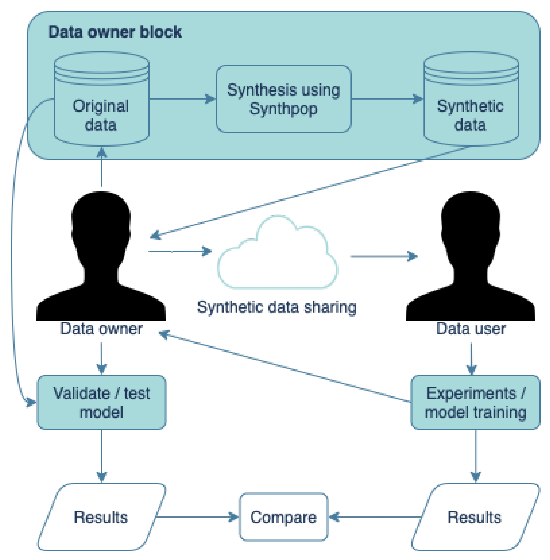
Current data-sharing systems, including SQLShare and DataHub, promote collaborative data analyses but fail to consolidate privacy-preserving prospects or means to manage sensitive data. Many other tools using AI methods, mainly GANs, have been developed which synthesize the data. Most AI-based data synthesis methods are designed to work on imaging data and do not work for microdata. Some do; however, either they are not free to use or come with limited access to the tool’s capacity, such as Tonic [26], Hazy [27], Datomize [28], and Mostly AI [29]. The synthpop package is an alternative to the previously mentioned methods for data synthesis. It is free to use and is capable of handling any microdata; there is no access limitation to the tool. It [30] was utilized in 2018; a synthesized version of highly sensitive data probing the role of ovulatory changes on sexual desire and behavior was publicly released [31]. The data set consists of 26 thousand of diary entries from women. Since sexual diaries are extremely sensitive and hard to anonymize completely, the data collector did not request consent from participants to make data publicly available but instead synthesized the data and made them publicly available for secondary data analysis. Figure 1 illustrates the data synthesis process for data sharing with data users and how synthetic data models can be verified and tested using original data by the data owner while maintaining the subject’s privacy. In this study, the performance of synthpop [30], which produced a synthetic version of data that is meant to be anonymous, was explored and examined by measuring the impacts of the data synthesis process.
3. Methodologies
3.1. Synthpop
The synthpop package was written as a part of the Synthetic Data Estimation for UK Longitudinal Studies (SYLLS) project to share the sensitive population-level data outside the setting where researchers held the original data set. Later, the synthpop package was altered to make it applicable to other data sets.
In this study, synthpop was the primary data anonymization and synthesis tool. It created a synthetic version of the original data while retaining its statistical properties and relationships between the variables. The achievement of anonymity relies on the assumption that there are no matching samples in the original and synthetic data sets; also, there are no samples with extreme values which could serve as unique identifiers. The method works by replacing some or all observed values by sampling from an appropriate probability distribution, conditional on the variable to be synthesized, the values from all previously synthesized columns of the original data set, and the fitted parameters of the conditional distribution (simple synthesis) or posterior predictive distribution of parameters (proper synthesis) while retaining the statistical properties of the original data set and relationships between the variables. By default, the syn() function produces one synthetic data set, but multiple data sets can be generated by setting the parameter m to a coveted number. An additional parameter, seed, can be used to fix the pseudo-random number generator to reproduce the same results. By default, syn() uses simple synthesis, but proper synthesis can be done by setting the proper argument to TRUE.
3.1.1. Methods for Synthesis
The synthpop tool consists of parametric and non-parametric methods [30]. Table 1 lists the methods currently implemented in synthpop. Each method generates synthetic values for each variable sequentially. Synthetic values are generated using the distribution of variables to be synthesized conditional on the distribution of previously observed synthetic and original variables called predictors. The default synthesis method is "cart" for all variables with predictors. It is a non-parametric method based on the classification and regression tree (CART) that is capable of handling any data. However, the first variable to be synthesized in the data set does not have a predictor, and it is a particular case where its values are by default generated by random sampling with replacement from original values ("sample" method). However, the user does not need to use the same synthesis method for all variables with predictors; a user can assign different methods from the list of methods to each variable in the data set, befitting the data type. On the other hand, setting the parameter method to "parametric" assigns default parametric methods to each variable based on its data type. Furthermore, if a user does not want to change or synthesize a variable, an empty method (" ") should be used for that variable. Finally, a new synthesis method can be defined by writing a function named syn.newmethod().
Implementation of methods: Let y denote an original data vector of length n, denote a matrix () of synthesized covariates, and x denote a matrix () of original covariate.
(1) Classification tree (syn.ctree) or classification and regression tree (syn.cart): It fits a classification or regression tree by binary recursive partitioning, followed by finding a terminal node for each . Finally, a donor from the node members is randomly drawn and takes that draw’s observed value as the synthetic value. The difference between syn.ctree and syn.cart is that they use functions from different packages. syn.ctree uses the ctree function from the party package, whereas syn.cart uses the rpart function from the rpart package. The selection of splitting variables and a stopping rule for the splitting process make them different from others.
(2) Random forest (syn.rf): It uses Breiman’s random forest algorithm for classification and regression [32]. Furthermore, It utilizes the randomForest function from the randomForest package.
(3) Bagging (syn.bag): It generates synthetic data using bagging by utilizing randomForest function from the randomForest package with the number of sampled predictors equal to the number of all predictors.
(4) Logistic regression (syn.logreg): It is used for the synthesis of binary variables by the non-Bayesian or approximate Bayesian logistic regression model. The non-Bayesian method first fits a logistic regression to the original data, then calculates the predicted inverse logits for synthesized covariates. Finally, compare the inverse logits to a random (0,1) deviation and obtain synthetic values. The approximate Bayesian method (for proper synthesis) repeats the same process as the non-Bayesian method with one additional step before computing inverse logits, drawing coefficients from a normal distribution with mean and variance estimated in the first step.
(5) Normal Linear regression preserving the marginal distribution (syn.normrank): First, synthetic values of normal deviates of the rank of the values in y are generated using the spread around the fitted linear regression line of normal deviates of rank given x. Then synthetic normal deviates of ranks are transformed to get synthetic ranks used to assign values from y. For proper synthesis, the regression coefficients are drawn from a normal distribution with mean and variance from the fitted model.
(6) Unordered polytomous regression (syn.polyreg): The synthetic categorical variables are generated by the polytomous regression model. First, it fits categorical responses as a multinomial model. Later, it computes predicted categories and finally adds appropriate noise to predictions. The algorithm uses the multinom function from the nnet package. Numerical variables are scaled before fitting to cover the range (0, 1).
3.1.2. Controlling the Sequence and Prediction
Synthetic values of each variable are generated from a joint distribution. The joint distribution is defined in terms of a series of conditional distributions. The values are imputed sequentially from the variable’s distribution to be synthesized conditionally on two distributions: (1) the distribution of all previously observed variables in the original data set, and (2) the distribution of all previously synthesized variables. This sequential process is, by default, automated, following the order of how variables appear in the data set (left to right). However, the order can be changed or specified for each variable by listing the indices of columns in the desired order to set parameter visit.sequence. If a user wishes not to synthesize a variable and not use it as a predictor, it should be removed from the visit.sequence.
Furthermore, if a user wishes not to synthesize a variable yet wishes to use the variable as one of the predictors for the synthesizing model, then an empty (" ") method should be used while keeping the variable in visit.sequence. Note that the variable(s) to be synthesized later in visit.sequence cannot be used as predictor(s) for variable(s) which appear before it. Though, variable(s) can explicitly be removed as predictor(s) for any specific variable(s) by updating the predictor.matrix.
3.1.3. Handling Data with Restricted and Missing Values
Relationships between variables can diversify significantly within a data set. Some variables can depend on each other or be tightly linked. As the goal of synthetic data is to mimic all original data characteristics, these restrictions should be preserved during the data synthesis process. For example, in a clinical data set, the variable containing information about the patient’s sibling’s clinical history is restricted to the variable containing information about whether the patient has siblings; this restriction needs to be addressed to get the best results from the synthesis process. When other variables determine the value for some case, the rule and corresponding values should be specified using rule and rvalues parameters.
Furthermore, if the data set has missing values and the values are defined with something other than the R missing data code NA, it should be specified in the cont.na parameter of the syn() function. Missing values in categorical variables are handled as additional categories. However, missing values in continuous variables are modeled in two steps. First, an auxiliary binary variable is synthesized to model whether a value is missing. If multiple types of missing values exist, an auxiliary categorical variable is created to record this. Second, a synthetic model is fitted to non-missing values, and synthetic values are generated for non-missing categories in the auxiliary variable. Finally, the auxiliary variable with non-missing values and zeros for remaining records is used to predict other variables.
3.2. Utility Measures of Data
The purpose of a synthetic data set is to resemble all the properties of the original data set. Thus, analyses made on synthetic data sets should lead to the same conclusions as those on the original data set. In theory, the model used for the synthesis process should resemble the original data-generation process to achieve its purpose. The methods to assess the utility of the synthetic data set can be broadly divided into general utility and specific utility [33]. The general utility estimates whether synthetic data have overall similarities in the statistical properties and multivariate relationships with the original data set. Simultaneously, the specific utility assesses the similitude of a fitted model’s performance on the synthetic data to its performance on the original data. The synthpop package provides two types of analyses for the synthetic data set based on the general and specific utility of the data set utilizing the compare() function in the package. First is the relative frequency distribution, and second is the linear machine learning model’s confidence interval overlap. However, due to the complexity of real-world microdata, especially for clinical microdata, more sophisticated tools to measure the impact of data anonymization are needed. As many real-world data, including clinical data, have non-linear relationships within their features; using a linear machine learning model to evaluate the machine learning capabilities of the synthetic data does not seem to be sufficient. Therefore, besides relative frequency distribution from the package and more rigorous analyses were performed in this study.
The overall utility of synthetic data is assessed on how adequately synthetic data succeed at all conducted utility tests, as detailed in Section 3.2.1. To succeed at a utility test, synthetic data need to resemble all the properties of original data, leaving no statistically significant difference. For formal assessments, the hypotheses are as follows: Let D denote an original data set, and represents a synthetic data set, where i indicates the index for synthetic data produced with the different synthesizing methods. Let t denote a vector of tests that returns a statistic and be a comparison function that returns a p-value. Finally, compare the output of with , a threshold value for the significance level.
The synthetic data quality was estimated based on whether utility tests led to rejecting the null hypothesis. To reject the null hypothesis, the comparative results using the comparison function () between original and synthetic data must have a p-value larger or equal to for all utility tests. The null hypothesis was not to be rejected if the comparative result using comparison function () between original and synthetic data possessed a p-value smaller than for any utility test. Note that the was set to for all tests.
3.2.1. General and Specific Utility Measures
The relative frequency distribution provides the fraction or proportion of times a value occurs in a data set. A side-by-side univariate distribution of each variable in the synthetic and original data set will be plotted to compare the probability distribution changes, which can be used to determine the likelihood of specific results occurring within a given population [30]. Two data sets can possess nearly identical statistical properties yet have very different distributions; therefore, the two-sample Kolmogorov–Smirnov test must be used to evaluate whether two underlying one-dimensional probability distribution differs in two different data sets (original and synthetic data set) for each variable.
Apart from visualizing frequency distributions, visualization of data points can help analysts look at data from a different perspective. Visualization of data directly, which has more than three dimensions, is currently out of scope. Still, dimension-reduction techniques that preserve the relationship between variables can be used as pre-steps. Uniform manifold approximation and projection (UMAP) is a dimension reduction technique that can be used for visualization similarly to T-distributed stochastic neighbor embedding (t-SNE) [34], but also for general non-linear dimension reduction [35]. UMAP is constructed from Riemannian geometry and an algebraic topology-based theoretical framework. The result is a scalable algorithm that applies to real-world data. Despite being similar to t-SNE, it is competitive for visualization quality and arguably preserves more of the global structure. Following the dimension reduction of the data while preserving global and local structures, data can be visualized in two or three dimensions.
The bivariate Pearson product-moment correlation coefficient (PPMCC) is a parametric measure of the linear correlation between pairs of continuous variables. PPMCC produces a sample correlation coefficient, R, which measures the linear relationship’s strength and direction. The PPMCC also evaluates whether there is significant statistical evidence for a linear relationship among the same pairs of variables, represented by a population correlation coefficient, (rho).
The specific utility of the data can be assessed by comparing the fitted synthetic and original models’ performances. This study used multiple machine learning models as classifiers, such as gradient boosting machine and random forest. Both of these methods can also be used for regression. Different types of machine learning models were used to evaluate the generality of the primary method of synthesis "synthpop". Moreover, the performance of the fitted model was examined based on multiple parameters for overall performance estimation.
Boosting algorithms were initially introduced by the machine learning community [36,37,38] for classification problems. The boosting algorithm’s principle approach combines several simple models iteratively, termed weak learners, to obtain a strong learner with improved predictive accuracy. A new statistical point of view for boosting was introduced to connect the boosting algorithm to the concept of loss functions [39]. Later, an extended boosting algorithm for regression termed the gradient boosting machine (GBM) was introduced [40]. The GBM is similar to a numerical optimization algorithm that aims to find an additive model that minimizes the loss function. Thus, GBM is a classification and regression forward-learning ensemble technique that generates a prediction model in the form of an ensemble of weak prediction models, typically decision trees that best reduce the loss function. This study follows the GBM algorithm implemented in the H2O package in R [41], which follows the algorithm specified by Hastie et al. [42].
Random forest classifier (RF) is a meta-estimator that fits several decision tree classifiers on various data sets sub-samples and uses the averaging approach to improve the predictive accuracy and control over the over-fitting [43]. In this study, Breiman’s random forest algorithm for classification implemented in scikit-learn 0.24.2 was used [32,43]. The performance of the fitted model was examined by multiple parameters, such as F1-score, receiver operating characteristic (ROC) curve, and accuracy, for overall performance estimation.
3.3. Quality of Information
The data-anonymization procedure aims to reduce semantics, meaning minimizing or removing personal information in a data set [44,45]. Data anonymization can cause distortion and information loss in the data set [44]. Entropy is a fundamental quantity in information theory associated with any random variable. Entropy can be interpreted as the level of information, surprise, or uncertainty associated with a random variable’s value or the result of a random process. The bit, which is the entropy unit, was adopted as a quantitative measure of information or a measure of surprise. The entropy of a random variable X, with possible outcomes , each with a probability of occurrence , is calculated as:
The entropy is maximal when all outcomes are equally likely in a system. The entropy goes down if the system moves away from equally possible outcomes or introduces some predictability. The information theory’s fundamental idea is that if the entropy of an information source, system, or data set drops, fewer questions are needed to guess the outcome. Entropy is directly proportional to uncertainty; i.e., as the value of entropy increases due to unpredictability, uncertainty in the system’s outcome increases, and the ability to compress decreases. Similarly, if the value for entropy decreases due to known structure, then the ability to compress increases, which leads to entropy being indirectly proportional to the ability to compress.
Mutual information (MI) is a measure of mutual dependence between two random variables. MI measures the information gain for a random variable X when information about another variable Y is given. MI between two random variables X and Y can be calculated as:
or
If entropy is a measure of uncertainty about a random variable Y, then is a measure of what X does not say about Y. In other words, is the uncertainty remaining about Y after X is known. Therefore, the equation can be interpreted as the amount of uncertainty in Y minus the amount of uncertainty in Y after X is known. Furthermore, this provides the inherent meaning of MI as the amount of information or reduction in uncertainty that one random variable provides about the other. Kraskov’s estimator [46] of mutual information is closely related to Shannon’s entropy, but Kraskov’s estimator relies on the nearest neighbors’ count. Kraskov’s estimator, along with many others [47], uses canonical distance defined in metric space for computability over Euclidean space and uses the Euclidean distance function. The mutual information estimator between two random variables and is defined as:
with being the digamma function and k denoting the number of neighbors. denotes the averages of both vectors and holding counts of neighbors overall [1, ..., N] and overall realizations of the random samples. In this study, a variation of the second algorithm from Kraskov’s estimator proposed by Oliver et al. [45] to use the method over non-Euclidean spaces using non-Euclidean distances was used. The calculation requires the nearest neighbors of points in joint space and counting how many lie in an absolute ball [45].
4. Experiments and Results
First, the performances of the different synthesis methods were evaluated based on the specific utility of the DIPP synthetic data set to select the fittest synthesis method. Specific utility compares the performances of the synthetic and original-data-fitted models. Following the method selection, general utility and the quality of information content were assessed for the selected synthetic data set. The general utility examines the statistical properties of the synthetic data set compared to the original data set based on the correlations among data variables, data visualization, data distributions, and data similarity. The quality of the information content is measured from an information-theoretic point of view, covering entropy and MI within the data sets. Similarly, all three primary analyses were repeated for the WDBC data set with the same motivation for general utility and quality of information contained in the data set but with additional motivations for specific utility experiments.
4.1. Specific and General Utility
The pre-processed version of the DIPP data set is a data frame with 30 attributes, including the binary response variable for 1329 subjects. Later, the data set was synthesized numerous times via the syn() command from the synthpop package using several methods. As mentioned earlier in Section 3.1.1, the first variable to be synthesized in the data is by default generated using the "sample" method. In our case, the response variable, "POS_antibodies", was the first to be synthesized, and then the rest of the attributes. For the reader interested in detailed implementation, Table A1 provides the list of all attributes in the data set and their descriptions in the order of synthesis, i.e., "visit.sequence".
Three different synthesis methods generated three synthetic data sets for initial experimentation. The methods used were "cart", "ctree", and "parametric"; and let SynD1, SynD2, and SynD3 denote generated synthetic data sets, respectively. One method of synthesis which performed the best out of those three methods was selected for generating another synthetic data set (SynD4) by setting the argument proper to TRUE for proper synthesis for further analysis.
The goal was twofold: first, to investigate if synthetic data sets can be used for machine learning problems when the original data cannot be acquired (due to patient’s privacy), and second, to assess how well synthetic data sets perform under a machine learning classifier as compared to the original data set. The machine learning classifier used was the GBM model, which was fitted, validated, and tested ten times (for more stable model performance) with all synthetic data sets and the original data set. Additionally, each data set was divided into three splits before model fitting: 75.0% of data for training, 12.5% for validation, and 12.5% for testing. We compared the results obtained from synthetic data test sets to the results of the original data test set to evaluate which synthesizing method produces the synthetic data set most resembling the performance of the original data set. The performance measure used was the confusion matrix and the parameters derived from it. The motivation behind using multiple performance parameters was to provide a more robust interpretation [48], as a model can have very high accuracy yet suffer from low precision [49] (pp. 128–129).
One sample set out of ten for the comparative performance of DIPP synthetic data sets (SynD1 to SynD4) with the original data set can be seen in Table 2. Note that the process was repeated ten times for all data sets to perform a significance test for testing accuracies. The accuracy of each synthetic data set-fitted model and of original data set-fitted model were compared using the comparison function. The function returns a p-value. Table 3 provides the p-value for each data set. Every single p-value was calculated using a t-test, comparing the accuracies of every synthetic data set to the original data set for the GBM model (10 iterations). Furthermore, a test set of original data sets was fed into the synthetic-data-fitted model to evaluate the local and global structure-preserving capabilities of the synthesis method and the pertinence of one aspect of the secondary data analysis. This comparative performance can also be seen in Table 2.
The objective was to reject the null hypothesis, i.e., the difference in the performance of the synthetic-data-fitted model should differ from the performance of the original-data-fitted model by, at the most, a non-significant amount. In other words, the aim is that the synthetic data set produced using any method does not perform better or worse than the original data. It must function as similar to the original data set as possible. From Table 3, the data sets produced using methods "cart" (SynD1) and "parametric" (SynD3) are the only data sets with p-values greater than , whereas the rest have p-values smaller than . If the p-value is greater than ; two data sets show enough evidence to reject the null hypothesis, meaning that the difference is statistically non-significant. Note that the p-value for each data set was calculated only using the accuracies of the model over the test set, which reflects the model’s generalizability. However, from Table 2, we can also say that SynD1 performs better than SynD3 when other evaluation parameters are considered. The overall performance difference from the original data is smaller for SynD1 than SynD3.
The analyses of SynD1 to SynD4 showed that the performance of SynD1 resembles that of the original the most. Therefore, the WDBC original data set was synthesized twice using the "cart" method. The whole data set was synthesized (SynW1), following only the training set being synthesized (SynW2), which was 30% of the data. As mentioned earlier in Section 3.1.1, the synthesis of the first variable in the data set by default uses the "sample" method, as it does not have a predictor. In our case, the binary response variable (M = malignant or B = benign) was the first to be synthesized; the rest of the attributes were synthesized in the order they would be found in the WDBC data set repository [9]. After synthesizing the original WDBC data set, SynW1 and SynW2 were preprocessed, and 14 highly correlated features were removed from all three data sets (original, SynW1, and SynW2)). The RF models were trained and tested three times in total with preprocessed original and synthetic data sets with 5-fold cross-validation. For all models, 70% of the data were used for training and 30% for testing.
In Table 2 is the performance list of original WDBC and SynW1 data-fitted models, along with the information about which data set was used for training and testing. Furthermore, a test set of original WDBC data sets was fed into the synthetic data (SynW2) fitted model to evaluate the local and global structure-preserving capability of the synthesis method and pertinence of one aspect of the secondary data analysis. The comparative performance can be seen in Table 2.
In Table 2 and Table 3, the results indicate that the synthetic data set (SynW1) performed similarly to the original data set. However, the performance of the SynW2 data-fitted model declined slightly when tested with the original data test set. Indeed, from the implementation of SynW2, we can say that the size of data affects the performance of the synthesis process, as the values are imputed by sampling from an assumed distribution. This experiment also shows that a model trained on synthetic data can be used to test for new original samples with success.
From the correlation matrix (Figure 2 and Figure 3), the original and synthetic data sets clearly have similar strong correlations between most variables. The relative frequency distributions analysis for the original and synthetic data sets (Figure 4 and Figure 5) report similar distributions between the original and synthetic data sets’ variables. The UMAP embedding for both original and synthetic data sets (Figure 6, Figure 7, Figure 8 and Figure 9) shows that samples belonging to each class form individual, similarly shaped clusters. However, the global structure of the WDBC synthetic data set is mirrored compared to the original data set in Figure 9. Furthermore, the data similarity between the original (DIPP and WDBC) and synthetic (SynD1 and SynW1) data sets of all discrete and continuous variables using the Kolmogorov–Smirnov two-sample test can be found in supplementary Table A2 and Table A3. A Kolmogorov–Smirnov two-sample test affirms that the analyses show evidence to reject the null hypothesis. That is, the variation in the distribution of these variables is statistically non-significant, as all attributes have a -value larger than .
4.2. Quality of Information
After analyzing the impacts of data synthesis and usability of data from a data mining point of view, the concepts of information theory were used further to evaluate the level of distortion in a data set and quantify the information loss. Claude Shannon’s entropy in bits, calculated for all variables concerning both original and synthetic data sets, reveals that a few variables in the synthetic data sets suffered a slight drop in entropy by approximately one bit, suggesting a probability of data compression, leading to a slight increase in the predictability of values for each data variable. A visual result of the entropy bit can be seen in supplementary Figure A1 and Figure A2. Finally, MI between all feature vectors and the response variable for both original and synthetic data sets was calculated using a variation of Kraskov’s estimation method. The distance between samples was calculated using a k-NN algorithm with three neighbors over a non-Euclidean space. The analysis found no variation in MI in the synthetic data sets compared to the original data sets, as the values of MI for both DIPP and WDBC synthetic data sets were the same positive numbers as for their corresponding original data sets, 12.786 and 10.239, respectively.
5. Conclusions and Discussion
It is natural to see clinical data suffering from imbalanced classes. This is often expected, as the data are not gathered in an experimental setting, such as a randomized controlled trial. It is necessary to note that such characteristics affect the performances of machine learning algorithms [50,51]. In our case, it was not the scope of this study to investigate this reasoning and improve the performance; however, it is essential, as it has also affected the data synthesis process. The tool imputes the values for synthetic variables from fitted parameters of synthesizing models, and imbalanced classes play a significant role in most synthesizing methods. The DIPP data set was pre-processed and mostly aggregated from a longitudinal database. When such data are generated, it is expected that the data set will suffer from imbalanced classes. Such characteristics play a significant role in data analysis; in our case, the effects can be seen in model training. Most synthetic-data-fitted models, including the original model, performed reasonably well in predicting negative and positive cases, despite having many negative samples. However, one synthetic data set (SynD3) significantly favored the negative samples more than any other data set. The SynD3 was the only synthetic data set produced using parametric methods fitting the data variable’s type. This analysis suggests that during data synthesis, model fitting parameters of the synthesizing method might have suffered overfitting, and synthetic data values were attributed to favoring negative classes. Even though the significance test of the accuracies of the SynD3 data-fitted model showed no statistically significant difference from that of the original-data-fitted model, when other evaluation parameters were considered, the SynD3 revealed various shortcomings favoring the previous finding. These interpretations underline the importance of the other evaluation parameters while determining a model’s performance.
Despite its weaknesses, the tool exceeded expectations when the default synthesis method "cart" (capable of handling any data type) was used. Two synthetic data sets were generated using the "cart" method: SynD1 and SynD4. The only difference was that SynD6 data were generated while setting the argument proper to TRUE for proper synthesis. Repeatedly, the SynD4 data-fitted model showed signs of overfitted parameters of the synthesizing model during data synthesis—however, the SynD1 data-fitted model outperformed in all analyses. The synthetic data set showed no signs of variation in data utility. The synthetic data set SynD1 succeeded in all performed tests with the statistically non-significant difference from the original data set; this is the only synthetic data set that led to rejecting the null hypothesis. Additionally, the quality of the information content was well preserved for 27 out of 30 variables. For the rest of the three variables, SynD1 suffered a decrease in entropy only by 1 bit. Conclusively, these analyses suggest that the "cart" method preserved not only the utilities but also the complexity of the DIPP data set according to the data standard established in this study, exhibiting that the tool certainly accomplished its intended goal.
The whole WDBC data set has undeniably strong correlations between features, since most are generated utilizing the initial ten real-valued features. Such a data set could be challenging to replicate fully, as similar variables are used to derive different features, and a strong dependence between the features is expected. Despite the complexity, the synthetic data set SynW1 succeeded in all performed tests by means of a statistically non-significant difference from the original data set; this is the only synthetic data set that led to rejecting the null hypothesis. Additionally, the quality of the information content was well preserved for all variables, except that SynW1 suffered a decrease in entropy only by 1 bit. Conclusively, these analyses suggest that the "cart" method preserved not only the utilities but also the complexity of the WDBC data set according to the data standard established in this study, exhibiting that the tool accomplished its intended goal. The overall performance of the data synthesis tool was remarkable. The tool performed adequately on all performed tests.
Overall, synthpop fulfills all the necessities and unfolds many opportunities for the research community, including easy data sharing, more significant collaborations, and information protection [52]. The impediments in clinical data mining and sharing most often relate to a research participant’s or patient’s privacy and security, and the circumstance that researchers face of having to consider the trade-off between the risk of disclosure and the benefits of open data sets [52,53,54,55]. Sharing clinical data could extend scientific collaboration for innovative discoveries and validate previously defined hypotheses. In numerous situations, the survival of data itself depends on the data holder’s capability to share data when needed, since not releasing data at all may eventually diminish the need for it [1]. Considering the workflow of the study, we can also state that data collectors and authors will always be indulged, since the findings from the synthetic data need verification from the original data set. This dependency on the original data set for result verification limited our study because the synthetic data can only be used for secondary data analysis. If the original author cannot be reached for result verification, the analyses may cease and result in an abandoned study. However, using synthetic data for secondary data analysis will enhance the collaboration between data owners and external data scientists while maintaining the subject’s privacy.
However, as demonstrated in this study, a user could utilize different tools to measure the utility of the data or consolidate further questioning if desired. By subsequently studying and assessing synthpop by measuring the impacts of the data synthesis process, we concluded that the tool performs competently in the current setting. Future researchers could consider testing the performance of synthpop by synthesizing the WDBC data set using different synthesis methods. Furthermore, implementing a more sophisticated way to read entropy bits and investigating the mutual information between pairs of variables in both original and synthetic data sets could highlight more in-depth impacts of the data synthesis process.
Author Contributions
Conceptualization, G.C.; methodology, G.C., P.S. and S.T.; software, G.C.; validation, G.C.; formal analysis, G.C.; investigation, G.C.; resources, G.C.; data curation, G.C., R.V. and M.J.K.; writing, G.C.; visualization, G.C.; supervision, P.S. and S.T.; project administration, P.S., S.T. and J.R.; funding acquisition, J.R. All authors have read and agreed to the published version of the manuscript.
Funding
This study is funded by the HTx project, which has received funding from the European Union’s Horizon 2020 research and innovation program under grant agreement No. 825162. HTx is a Horizon 2020 project supported by the European Union, lasting five years from January 2019. The main aim of HTx is to create a framework for the Next Generation Health Technology Assessment (HTA) to support patient-centered, societally oriented, real-time decision making regarding access to and reimbursement for health technologies throughout Europe.
Institutional Review Board Statement
Ethical review and approval were waived for this study as the study did not include any data gathering, it was based on previously collected data.
Informed Consent Statement
Patient consent was waived due to an open data set.
Data Availability Statement
More information on DIPP data and its owners can be found on the DIPP data website: http://dipp.fi (accessed on 4 December 2022). WDBC data supporting reported results can be found in [9,56] and links to the data set analyzed: https://archive.ics.uci.edu/ml/datasets/breast+cancer+wisconsin+(diagnostic) (accessed on 4 December 2022).
Acknowledgments
This article is based on my master thesis [57]. I want to express my most profound appreciation to my supervisor Pekka Siirtola and reviewer, Satu Tamminen, for their constructive feedback, patience, and valued guidance. I want to thank Ian Oliver and his team for presenting me with the background concerning the mutual information analyses. Finally, I thank my research group leader Juha Röning for his support and encouragement.
Conflicts of Interest
The authors declare no conflict of interest. The funders had no role in the design of the study; in the collection, analyses, or interpretation of data; in the writing of the manuscript; or in the decision to publish the results.
Abbreviations
The following abbreviations are used in this manuscript:
| CART | Classification And Regression Tree |
| DIPP | Finnish Type 1 Diabetes Prediction and Prevention study database |
| EHR | Electronic Health Records |
| FN | False Negative |
| FP | False Positive |
| GAN | Generative adversarial networks |
| GBM | Gradient Boosting Machine |
| GDPR | General Data Protection Regulation |
| k-NN | k-Nearest Neighbor |
| MI | Mutual Information |
| ML | Machine Learning |
| PPMCC | Pearson product-moment correlation coefficient |
| RF | Random Forest |
| ROC | Receiver Operating Characteristic |
| SYLLS | Synthetic Data Estimation for UK Longitudinal Studies |
| TN | True Negative |
| TP | True Positive |
| t-SNE | T-distributed Stochastic Neighbor Embedding |
| UMAP | Uniform Manifold Approximation and Projection |
| WDBC | Wisconsin Diagnostic Breast Cancer data set |
Appendix A
This Appendix section outlines the structure and objective of each data set used in this study along with miscellaneous results.
Appendix A.1. Wisconsin Diagnostic Breast Cancer Data Set
Breast cancer is the second most common cause of death in American women who are 40 to 55 years of age [58]. Since the 1930s, the beginning of formal tracking of cases through the registry, breast cancer rates have been regularly increasing in the United States [58]. Many researchers worldwide have been studying and trying to detect breast cancer early in life to decrease the mortality rate.
The WDBC data set used in this study is an open data set, which implies that the data is free and available at the University of California Irvine Machine Learning Repository [9]. The motivation for using the WDBC data set in this study is to utilize a different and more complex data set consisting of a relatively high correlation between variables. The data set features were derived from ten real-value features, which caused a high correlation within the data set. Furthermore, the data set is openly available, so the findings from this study can be replicated or further questioned, supporting the study’s primary objective. Therefore, this study examined the performance of the data synthesis tool over the WDBC data set toward the possibility of data sharing for similar data sets.
The data set has 569 samples with 32 attributes, including ID, diagnosis, and 30 real-valued input features. The diagnosis is binary, either M = malignant or B = benign. Ten real-valued features were computed for each cell nucleus:
- radius (mean of distances from the center to points on the perimeter)
- texture (standard deviation of grey-scale values)
- perimeter
- area
- smoothness (local variation in radius lengths)
- compactness (perimeter/area − 1.0)
- concavity (severity of concave portions of the contour)
- concave points (number of concave portions of the contour)
- symmetry
- fractal dimension ("coastline approximation" − 1)
Furthermore, for each of these features, mean, standard error, "worst," or largest (mean of the three largest values) were computed for each image, resulting in 30 features. Finally, the class distribution is 357 for benign and 212 for malignant.
Type 1 Diabetes Prediction and Prevention Data Set
Finland has the highest incidence of Type 1 Diabetes (T1D) in the world amongst young children, currently standing at approximately 72 in every 100,000 children under the age of 15 years [59]. The DIPP Study was established in 1994 in three university hospitals in Finland to understand/learn the pathogenesis of T1D [8]. This ongoing study aims to find new treatments and preventative methods by assessing risk factors in the development of T1D. The DIPP study is a population-based long-term clinical follow-up study that involves screening newborns for increased genetic risk for diabetes.
The DIPP database used in this study has been collected since 1994 only at the Oulu University Hospital. It contains information from over 6500 subjects in the form of longitudinal data recorded since birth. The database includes information about the subject, siblings, and parents’ monitoring information. The database also suffers from missing values due to non-standardized input methods, such as information entered by hand during collection. The database comprises blood samples, infections, medications, vaccines, nutrition, and environmental factors. Blood sample data includes three autoantibody values of glutamic acid decarboxylase (GADA), protein tyrosine phosphate autoantibody (IA2A), and antibodies of insulin (IAA).
The data set used in this study was built and pre-processed from the original DIPP database. Until 12 months, the data were aggregated to utilize information gained from that data to predict the positivity of the autoantibodies later in life. First, variables such as infections were aggregated to value 0 if the number of infections is zero or to value 1 if more than one or two infections in the first 12 months of age. Infections leading to hospital care and other similar variable were cumulated similarly. Furthermore, for variables such as autoantibodies, the maximum autoantibody value was taken into account before the first positive value of 12 months of age occurred. Later, seven subjects whose autoantibodies were in the positive range before 12 months of age due to autoantibodies transmitted from the mother were excluded. Finally, a response variable "POS_antibodies" was defined based on autoantibodies’ positivity. The class negative is if the subject never had an occurrence of positive value in any autoantibodies up until 170 months of age, and class positive is if the subject had two or more consecutive positive value occurrences in any autoantibodies up until 170 months of age. An autoantibody’s value is positive if they were higher than a specific threshold for the respective autoantibodies. The threshold values for GADA, IA2A, and IAA are 5.34, 0.42, and 3.47, respectively. Overall, there are 30 attributes using a small subset of data of 1329 subjects. Of these, 839 subjects belong to the positive and 490 to the negative classes. Table A1 provides a list of all the data set attributes and their description. The data set’s goal is to predict the probability of the positivity of autoantibodies before the age of 15 by utilizing information gained from the first 12 months of data.

Table A1.
Names and descriptions of attributes for the DIPP data set.
| Attributes | Description |
|---|---|
| POS_antibodies | Response variable— 1 the child had two or more consecutive positive samples in any of the auto-antibodies, 0 otherwise |
| length | Length at birth (cm) |
| weight | Weight at birth (g) |
| circle_of_head | Head circumference measured at birth (cm) |
| ratio_head_length | Ratio between head circumference and length measured at birth (cm) |
| Mom_birth_age | Age of mother at the time of birth (years) |
| height_growth | Growth rate calculated by: (height measured in the last visit—length at birth)/Age in months |
| weight_growth | Growth rate calculated by: (weight measured in the last visit—birth weight/1000)/Age in months |
| GADA.UUSI | Maximum value of GADA antibody that occurred before 12 months old (negative value) |
| mIAA.3.470 | Maximum value of IAA antibody that occurred before 12 months old (negative value) |
| IAA.0.42 | Maximum value of IA2A antibody that occurred before 12 months old (negative value) |
| s.gender | Gender 1—male, 2—female |
| duration | Pregnancy duration: 0—pre term 0 to 37 weeks, 1—normal 37 to 42 weeks, 2—post-term > 42 weeks |
| month | Month of birth—from 1 to 12 |
| mother_antib | 1—if the child’s mother had positive autoantibodies, 0 otherwise |
| sibling_antib | 1—if the child’s sibling had positive autoantibodies, 0 otherwise |
| has_sibling | 1—if the child has siblings, 0 otherwise |
| is_mom_t1d | Does mom have t1d 1—yes, 0—no |
| is_dad_t1d | Does dad have t1d 1—yes, 0—no |
| v.breastfeeding_only | Age when exclusive breastfeeding has ended (months) |
| v.breastfeeding_ended | Age when any breastfeeding has ended (months)—maximum is 12, which means currently still breastfeeding. |
| i.infections_ear | 0—no ear infections, 1—1 infection, 2—more than 2 infections |
| i.infections_eye | 0—no eye infections, 1—more than 1 infections |
| i.infections_hospital_care | 0—no infections requiring a hospital stay, 1—more than 1 infections |
| i.infections_airway | 0—no airway infections, 1—1 infection, 2—more than 2 infections |
| i.infections_gastric | 0—no infections, 1—1 or more infections |
| i.infections_other | |
| i.infections_fever | |
| i.infections_roseola | |
| i.infections_chickenpox |
Appendix A.2. Miscellaneous Results
Table A2.
-value and Cucconi p-value for matching continuous and discrete attributes between original and SynD1 data sets.
Table A2.
-value and Cucconi p-value for matching continuous and discrete attributes between original and SynD1 data sets.
| Attribute | KSp-Value | Cucconi p-Value |
|---|---|---|
| length | 0.7170990 | 0.603 |
| weight | 0.7924978 | 0.403 |
| circle_of_head | 1.0000000 | 0.914 |
| ratio_head_length | 0.9937073 | 0.495 |
| Mom_birth_age | 0.8930451 | 0.437 |
| height_growth | 0.9438003 | 0.629 |
| weight_growth | 0.7464065 | 0.472 |
| GADA.UUSI | 0.8380866 | 0.784 |
| mIAA.3.470 | 0.5239224 | 0.965 |
| IA2A.0.42 | 0.8097315 | 0.383 |
| month | 0.4346488 | 0.167 |
| v.breastfeeding_only | 0.9999954 | 0.946 |
| v.breastfeeding_ended | 0.9916316 | 0.981 |
Table A3.
-value for matching continuous and discrete attributes between original and synthetic data sets.
Table A3.
-value for matching continuous and discrete attributes between original and synthetic data sets.
| Attribute | KSp-Value |
|---|---|
| radius_mean | 0.9613699 |
| texture_mean | 0.9089228 |
| perimeter_mean | 0.9613699 |
| area_mean | 0.9383389 |
| smoothness_mean | 0.5924107 |
| compactness_mean | 0.9999932 |
| concavity_mean | 0.9780573 |
| concave.point_mean | 0.9613699 |
| symmetry_mean | 0.8735816 |
| fractal_dimension_mean | 0.9890057 |
| radius_se | 0.8735816 |
| texture_se | 0.9890057 |
| perimeter_se | 0.9613699 |
| area_se | 0.8735816 |
| smoothness_se | 0.2048226 |
| compactness_se | 0.9983954 |
| concavity_se | 0.9780573 |
| concave.point_se | 0.4076697 |
| symmetry_se | 0.6921113 |
| fractal_dimension_se | 0.9613699 |
| radius_worst | 0.9089228 |
| texture_worst | 0.9995891 |
| perimeter_worst | 0.6421872 |
| area_worst | 0.8735816 |
| smoothness_worst | 0.4507638 |
| compactness_worst | 0.9383389 |
| concavity_worst | 0.9953208 |
| concave.point_worst | 0.9983954 |
| symmetry_worst | 0.7412813 |
| fractal_dimension_worst | 0.9953208 |
Figure A1.
Entropy per bit for original and SynD1 data variables.

Figure A2.
Entropy per bit for original and synthetic data variables.

References
- Sweeney, L. k-anonymity: A model for protecting privacy. Int. J. Uncertain. Fuzziness Knowl.-Based Syst. 2002, 10, 557–570. [Google Scholar] [CrossRef] [Green Version]
- Viceconti, M.; Hunter, P.; Hose, R. Big data, big knowledge: Big data for personalized healthcare. IEEE J. Biomed. Health Inform. 2015, 19, 1209–1215. [Google Scholar] [CrossRef] [PubMed]
- Ohm, P. Broken promises of privacy: Responding to the surprising failure of anonymization. UCLA Law Rev. 2009, 57, 1701. [Google Scholar]
- Huston, P.; Edge, V.; Bernier, E. Open Science/Open Data: Reaping the benefits of Open Data in public health. Can. Commun. Dis. Rep. 2019, 45, 252. [Google Scholar] [CrossRef] [PubMed]
- Singh, K.N.M.; Shetty, Y.C. Data sharing: A viable resource for future. Perspect. Clin. Res. 2017, 8, 63. [Google Scholar] [CrossRef] [PubMed]
- Devriendt, T.; Borry, P.; Shabani, M. Factors that influence data sharing through data sharing platforms: A qualitative study on the views and experiences of cohort holders and platform developers. PLoS ONE 2021, 16, e0254202. [Google Scholar] [CrossRef]
- Yale, A.; Dash, S.; Dutta, R.; Guyon, I.; Pavao, A.; Bennett, K.P. Privacy Preserving Synthetic Health Data. In Proceedings of the 2019 ESANN, European Symposium on Artificial Neural Networks, Computational Intelligence and Machine Learning, Bruges, Belgium, 24–26April 2019; pp. 465–470. [Google Scholar]
- Finnish Type 1 Diabetes Prediction and Prevention. Available online: http://dipp.fi (accessed on 21 October 2022).
- Wolberg, W.H.; Mangasarian, O.L. Multisurface method of pattern separation for medical diagnosis applied to breast cytology. Proc. Natl. Acad. Sci. USA 1990, 87, 9193–9196. [Google Scholar] [CrossRef] [Green Version]
- Van Ginneken, A.M. The computerized patient record: Balancing effort and benefit. Int. J. Med. Inform. 2002, 65, 97–119. [Google Scholar] [CrossRef]
- Lee, J.; Park, Y.T.; Park, Y.R.; Lee, J.H. Review of national-level personal health records in advanced countries. Healthc. Inform. Res. 2021, 27, 102–109. [Google Scholar] [CrossRef]
- Kim, E.; Rubinstein, S.M.; Nead, K.T.; Wojcieszynski, A.P.; Gabriel, P.E.; Warner, J.L. The evolving use of electronic health records (EHR) for research. In Proceedings of the Seminars in Radiation Oncology; Elsevier: Amsterdam, The Netherlands, 2019; Volume 29, pp. 354–361. [Google Scholar]
- El Emam, K.; Jonker, E.; Arbuckle, L.; Malin, B. A systematic review of re-identification attacks on health data. PLoS ONE 2011, 6, e28071. [Google Scholar] [CrossRef] [Green Version]
- Greely, H.T. The Uneasy Ethical and Legal Underpinnings of Large-Scale Genomic Biobanks. Annu. Rev. Genom. Hum. Genet. 2007, 8, 343–364. [Google Scholar] [CrossRef]
- Fellegi, I.P. On the question of statistical confidentiality. J. Am. Stat. Assoc. 1972, 67, 7–18. [Google Scholar] [CrossRef]
- Denning, D.E. Secure statistical databases with random sample queries. ACM Trans. Database Syst. (TODS) 1980, 5, 295. [Google Scholar] [CrossRef] [Green Version]
- Samarati, P.; Sweeney, L. Protecting Privacy When Disclosing Information: K-Anonymity and Its Enforcement through Generalization and Suppression; Technical Report SRI-CSL-98-04; SRI Computer Science Laboratory: Palo Alto, CA, USA, 1998. [Google Scholar]
- Machanavajjhala, A.; Kifer, D.; Gehrke, J.; Venkitasubramaniam, M. L-diversity: Privacy beyond k-anonymity. Assoc. Comput. Mach. Trans. Knowl. Discov. Data 2007, 1, 3-es. [Google Scholar] [CrossRef]
- Li, N.; Li, T.; Venkatasubramanian, S. t-closeness: Privacy beyond k-anonymity and l-diversity. In Proceedings of the 2007 IEEE, 23rd International Conference on Data Engineering, Istanbul, Turkey, 15–20 April 2007; pp. 106–115. [Google Scholar] [CrossRef] [Green Version]
- Dwork, C.; McSherry, F.; Nissim, K.; Smith, A. Calibrating noise to sensitivity in private data analysis. In Proceedings of the Theory of Cryptography Conference; Springer: Berlin/Heidelberg, Germany, 2006; pp. 265–284. [Google Scholar] [CrossRef] [Green Version]
- Erlingsson, Ú.; Pihur, V.; Korolova, A. Rappor: Randomized aggregatable privacy-preserving ordinal response. In Proceedings of the 2014 ACM, Special Interest Group on Security, Audit and Control (SIGSAC) Conference on Computer and Communications Security, Scottsdale, AZ, USA, 3–7 November 2014; pp. 1054–1067. [Google Scholar] [CrossRef] [Green Version]
- Press, I.A. Apple Previews iOS 10, the Biggest iOS Release Ever. 2016. Available online: https://www.apple.com/newsroom/2016/06/apple-previews-ios-10-biggest-ios-release-ever/ (accessed on 4 December 2022).
- Muralidhar, K.; Domingo-Ferrer, J.; Martínez, S. epsilon-Differential Privacy for Microdata Releases Does Not Guarantee Confidentiality (Let Alone Utility). In Proceedings of the International Conference on Privacy in Statistical Databases; Springer: Cham, Switzerland, 2020; pp. 21–31. [Google Scholar]
- Culnane, C.; Rubinstein, B.I.; Teague, V. Health data in an open world. arXiv 2017, arXiv:1712.05627v1. [Google Scholar]
- gdpr.eu. General Data Protection Regulation. 2020. Available online: https://gdpr.eu (accessed on 4 December 2022).
- Tonic. The Fake Data Company. Available online: https://www.tonic.ai (accessed on 4 December 2022).
- Hazy Limited. Synthetic Data. Real Results. 2022. Available online: https://hazy.com (accessed on 4 December 2022).
- Datomize. Limited Data. Unlimited Insights. 2020. Available online: https://www.datomize.com (accessed on 4 December 2022).
- Mostly AI. Smarter Synthetic Data. Available online: https://mostly.ai (accessed on 4 December 2022).
- Nowok, B.; Raab, G.M.; Dibben, C. Synthpop: Bespoke creation of synthetic data in R. J. Stat. Softw. 2016, 74, 1–26. [Google Scholar] [CrossRef] [Green Version]
- Arslan, R.C.; Schilling, K.M.; Gerlach, T.M.; Penke, L. Using 26,000 diary entries to show ovulatory changes in sexual desire and behavior. J. Personal. Soc. Psychol. 2018, 121, 410. [Google Scholar] [CrossRef]
- Breiman, L. Random forests. Mach. Learn. 2001, 45, 5–32. [Google Scholar] [CrossRef] [Green Version]
- Snoke, J.; Raab, G.; Nowok, B.; Dibben, C.; Slavkovic, A. General and specific utility measures for synthetic data. J. R. Stat. Soc. Ser. A Stat. Soc. 2018, 181, 663–688. [Google Scholar] [CrossRef]
- Maaten, L.v.d.; Hinton, G. Visualizing data using t-SNE. J. Mach. Learn. Res. 2008, 9, 2579–2605. [Google Scholar]
- McInnes, L.; Healy, J.; Melville, J. Umap: Uniform manifold approximation and projection for dimension reduction. arXiv 2018, arXiv:1802.03426v2. [Google Scholar]
- Schapire, R.E. The strength of weak learnability. Mach. Learn. 1990, 5, 197–227. [Google Scholar] [CrossRef] [Green Version]
- Freund, Y. Boosting a weak learning algorithm by majority. Inf. Comput. 1995, 121, 256–285. [Google Scholar] [CrossRef] [Green Version]
- Freund, Y.; Schapire, R.E. Experiments with a new boosting algorithm. In Proceedings of the 13th International Conference proceedings, Machine Learning, San Francisco, CA, USA, 3–6 July 1996; pp. 148–156. [Google Scholar]
- Friedman, J.; Hastie, T.; Tibshirani, R. Additive logistic regression: A statistical view of boosting (with discussion and a rejoinder by the authors). Ann. Stat. 2000, 28, 337–407. [Google Scholar] [CrossRef]
- Friedman, J.H. Greedy function approximation: A gradient boosting machine. Ann. Stat. 2001, 29, 1189–1232. [Google Scholar] [CrossRef]
- Click, C.; Malohlava, M.; Candel, A.; Roark, H.; Parmar, V. Gradient boosting machine with H2O. H2O AI 2017. [Google Scholar]
- Friedman, J.; Hastie, T.; Tibshirani, R. The Elements of Statistical Learning; Springer Series in Statistics New York; Springer: Berlin/Heidelberg, Germany, 2001. [Google Scholar]
- Pedregosa, F.; Varoquaux, G.; Gramfort, A.; Michel, V.; Thirion, B.; Grisel, O.; Blondel, M.; Prettenhofer, P.; Weiss, R.; Dubourg, V.; et al. Scikit-learn: Machine Learning in Python. J. Mach. Learn. Res. 2011, 12, 2825–2830. [Google Scholar]
- Oliver, D.I. Privacy Engineering: A Dataflow and Ontological Approach; CreateSpace Independent Publishing Platform: North Charleston, SC, USA, 2014. [Google Scholar]
- Oliver, I.; Miche, Y. On the development of a metric for quality of information content over anonymised data-sets. In Proceedings of the 2016 IEEE, 10th International Conference on the Quality of Information and Communications Technology (QUATIC), Lisbon, Portugal, 6–9 September 2016; pp. 185–190. [Google Scholar] [CrossRef]
- Kraskov, A.; Stögbauer, H.; Grassberger, P. Estimating mutual information. Phys. Rev. E 2004, 69, 066138. [Google Scholar] [CrossRef] [Green Version]
- Pál, D.; Póczos, B.; Szepesvári, C. Estimation of Rényi entropy and mutual information based on generalized nearest-neighbor graphs. Adv. Neural Inf. Process. Syst. 2010, 23, 1849–1857. [Google Scholar]
- Tharwat, A. Classification assessment methods. Appl. Comput. Inform. 2018, 17, 168–192. [Google Scholar] [CrossRef]
- Taylor, J. Introduction to Error Analysis, The Study of Uncertainties in Physical Measurements; University Science Book: Mill Valley, CA, USA, 1997. [Google Scholar]
- He, H.; Ma, Y. Imbalanced Learning: Foundations, Algorithms, and Applications; John Wiley & Sons: Hoboken, NJ, USA, 2013. [Google Scholar]
- He, H.; Garcia, E.A. Learning from Imbalanced Data. IEEE Trans. Knowl. Data Eng. 2009, 21, 1263–1284. [Google Scholar]
- Quintana, D. Synthetic datasets: A non-technical primer for the behavioural sciences to promote reproducibility and hypothesis-generation. PsyArXiv 2019. [Google Scholar] [CrossRef]
- Cios, K.J.; Moore, G.W. Uniqueness of medical data mining. Artif. Intell. Med. 2002, 26, 1–24. [Google Scholar] [CrossRef]
- Lenert, L.; McSwain, B.Y. Balancing health privacy, health information exchange and research in the context of the COVID-19 pandemic. J. Am. Med. Inform. Assoc. 2020, 27, 963–966. [Google Scholar] [CrossRef]
- Ienca, M.; Vayena, E. On the responsible use of digital data to tackle the COVID-19 pandemic. Nat. Med. 2020, 26, 463–464. [Google Scholar] [CrossRef] [Green Version]
- Dua, D.; Graff, C. UCI Machine Learning Repository. 2017. Available online: https://archive.ics.uci.edu/ml/index.php (accessed on 4 December 2022).
- Chandra, G. Impacts of Data Synthesis: A Metric for Quantifiable Data Standards and Performances. Master’s Thesis, University of Oulu, Oulu, Finland, 2020. [Google Scholar]
- Harris, J.R.; Lippman, M.E.; Veronesi, U.; Willett, W. Breast cancer. N. Engl. J. Med. 1992, 327, 319–328. [Google Scholar] [CrossRef]
- Diabetesliitto. Finnish Diabetes Association. 2020. Available online: https://www.diabetes.fi (accessed on 4 December 2022).
Figure 1.
Data synthesis, sharing, and testing use case.

Figure 2.
Pearson correlation for original data set in the “lower” triangle and SynD1 data set in the “upper” triangle.
Figure 2.
Pearson correlation for original data set in the “lower” triangle and SynD1 data set in the “upper” triangle.

Figure 3.
Pearson correlation for original data set in the “lower” triangle and SynW1 data set in the “upper” triangle.
Figure 3.
Pearson correlation for original data set in the “lower” triangle and SynW1 data set in the “upper” triangle.

Figure 4.
Relative frequency distributions of a few original (observed) and SynD1 (synthetic) data set variables.
Figure 4.
Relative frequency distributions of a few original (observed) and SynD1 (synthetic) data set variables.

Figure 5.
Relative frequency distribution of a few original (observed) and SynW1 (synthetic) data set variables.
Figure 5.
Relative frequency distribution of a few original (observed) and SynW1 (synthetic) data set variables.

Figure 6.
Uniform Manifold Approximation and Projection for original DIPP data set.

Figure 7.
Uniform Manifold Approximation and Projection for SynD1 data set.

Figure 8.
Uniform Manifold Approximation and Projection for original WDBC data set.

Figure 9.
Uniform Manifold Approximation and Projection for SynW1 data set.

Table 1.
Built-in synthesizing methods. * Indicates default parametric methods [30].
Table 1.
Built-in synthesizing methods. * Indicates default parametric methods [30].
| Method | Description | Data Type |
|---|---|---|
| Non-parametric | ||
| ctree, cart | Classification and regression trees | Any |
| surv.ctree | Classification and regression trees | Duration |
| Parametric | ||
| norm | Normal linear regression | Numeric |
| normrank * | Normal linear regression preserving | Numeric |
| the marginal distribution | ||
| logreg * | Logistic regression | Binary |
| polyreg * | Polytomous logistic regression | Factor, >2 levels |
| polr * | Ordered polygamous logistic regression | Ordered factor, >2 levels |
| pmm | Predictive mean matching | Numeric |
| Other | ||
| sample | Random sample from the observed data | Any |
| passive | Function of the other synthesized data | Any |
Table 2.
Original and synthetic data sets and their performances using ML models.
| Test Set | Training Set | Predicted Labels | F1 Score | ROC Curve | ||
|---|---|---|---|---|---|---|
| Negative | Positive | |||||
| Original | Original | Negative | 89 | 16 | 0.85 | |
| DIPP | DIPP | Positive | 5 | 56 | 0.82 | 0.95 |
| Negative | 83 | 19 | 0.88 | |||
| SynD1 | SynD1 | Positive | 1 | 63 | 0.85 | 0.93 |
| Negative | 82 | 20 | 0.87 | |||
| SynD2 | SynD2 | Positive | 3 | 61 | 0.82 | 0.93 |
| Negative | 98 | 4 | 0.85 | |||
| SynD3 | SynD3 | Positive | 14 | 49 | 0.78 | 0.92 |
| Negative | 83 | 18 | 0.86 | |||
| SynD4 | SynD4 | Positive | 0 | 65 | 0.89 | 0.95 |
| Original | Original | Negative | 113 | 2 | 0.98 | |
| WDBC | WDBC | Positive | 3 | 53 | 0.95 | 0.96 |
| Negative | 111 | 2 | 0.98 | |||
| SynW1 | SynW1 | Positive | 2 | 56 | 0.97 | 0.97 |
| Original | Negative | 102 | 5 | 0.94 | ||
| WDBC | SynW2 | Positive | 7 | 57 | 0.90 | 0.92 |
Table 3.
p-values using accuracy from comparison function () between synthetic and original data sets.
Table 3.
p-values using accuracy from comparison function () between synthetic and original data sets.
| Data Set | p-Value |
|---|---|
| SynD1 | 0.0965496 |
| SynD2 | 0.0485093 |
| SynD3 | 0.1755973 |
| SynD4 | 0.0006553 |
| SynW1 | 0.0837001 |
Publisher’s Note: MDPI stays neutral with regard to jurisdictional claims in published maps and institutional affiliations. |
© 2022 by the authors. Licensee MDPI, Basel, Switzerland. This article is an open access article distributed under the terms and conditions of the Creative Commons Attribution (CC BY) license (https://creativecommons.org/licenses/by/4.0/).
Share and Cite
MDPI and ACS Style
Chandra, G.; Siirtola, P.; Tamminen, S.; Knip, M.J.; Veijola, R.; Röning, J. Impacts of Data Synthesis: A Metric for Quantifiable Data Standards and Performances. Data 2022, 7, 178. https://doi.org/10.3390/data7120178
AMA Style
Chandra G, Siirtola P, Tamminen S, Knip MJ, Veijola R, Röning J. Impacts of Data Synthesis: A Metric for Quantifiable Data Standards and Performances. Data. 2022; 7(12):178. https://doi.org/10.3390/data7120178
Chicago/Turabian StyleChandra, Gunjan, Pekka Siirtola, Satu Tamminen, Mikael J. Knip, Riitta Veijola, and Juha Röning. 2022. "Impacts of Data Synthesis: A Metric for Quantifiable Data Standards and Performances" Data 7, no. 12: 178. https://doi.org/10.3390/data7120178