A Comprehensive Data Pipeline for Comparing the Effects of Momentum on Sports Leagues

Abstract

Momentum has been a consistently studied aspect of sports science for decades. Among the established literature, there has, at times, been a discrepancy between conclusions. However, if momentum is indeed an actual phenomenon, it would affect all aspects of sports, from player evaluation to pre-game prediction and betting. Therefore, using momentum-based features that quantify a team’s linear trend of play, we develop a data pipeline that uses a small sample of recent games to assess teams’ quality of play and measure the predictive power of momentum-based features versus the predictive power of more traditional frequency-based features across several leagues using several machine learning techniques. More precisely, we use our pipeline to determine the differences in the predictive power of momentum-based features and standard statistical features for the National Hockey League (NHL), National Basketball Association (NBA), and five major first-division European football leagues. Our findings show little evidence that momentum has superior predictive power in the NBA. Still, we found some instances of the effects of momentum on the NHL that produced better pre-game predictors, whereas we view a similar trend in European football/soccer. Our results indicate that momentum-based features combined with frequency-based features could improve pre-game prediction models and that, in the future, momentum should be studied more from a feature/performance indicator point-of-view and less from the view of the dependence of sequential outcomes, thus attempting to distance momentum from the binary view of winning and losing.

1. Introduction

By the year 2027, the revenue for the global sports market is estimated to reach USD 623.63 billion. This is a marked increase from the revenue of USD 486.61 billion seen in 20221. This significant revenue growth also increases financial incentives for management groups to attempt to create successful sports franchises. One of the ways to improve a franchise is through the team’s quality of play, which has given rise to the use of sports analytics. Sports analytics are built on the idea that statistics, data science, and machine learning can improve a team’s quality by allowing management to make informed decisions with the use of information about the in-game play that the average scout, coach, or person in management may not notice by simply watching games.

The acceptance of sports analytics by fans, players, or people in management has often been slow and met with skepticism. In other cases, teams have embraced analytics and prospered because of it. Such was the case for the 2002 Oakland Athletics, who managed to create a competitive Major League Baseball (MLB) team at a fraction of the cost of their more wealthy competitors; this event became more colloquially known as “Moneyball” [1]. Due to this success, the field of sports analytics has grown to the point that many sports teams have in-house analytics departments. There is also a third-party market in which companies work with professional sports teams to provide in-depth statistical analysis or give them the tools to do so internally. Examples of such companies include Wyscout2, StatsBomb3, and Sportslogiq4.

Recently, a growing body of literature in sports analytics is interested mainly in studying the claims of many coaches, players, and fans that momentum impacts the outcome of the game [2]. These papers often conclude that momentum, as it is traditionally defined, does not exist in team sports [3,4]. In recent years, several papers have come to the opposite conclusion, stating that momentum impacts team sports [5,6]. In reviewing the literature on data engineering in sports analytics, we found a gap in the research. That gap is in providing a comprehensive approach to building a generic data pipeline using game events, from which valuable features can be extracted from event data. In this work, we try to fill this gap as follows. First, we propose a way to extract distinct sets of features from the event data to use later to evaluate their predictive power; this allows us to evaluate the effect (or lack thereof) of momentum on a given sport. We define momentum as the increase or decrease in a team’s overall quality of play over a small sample of games. Previous literature has often defined momentum differently. For instance, Arkes and Martinez [7] focused on momentum over multiple games and defined the effect of momentum as a “situation in which a team has a higher probability of winning or success had the team been playing well in the last few games”. Fry and Shukairy [8] studied momentum more from an in-game perspective and defined it as the idea that “certain positive (negative) events during a game cause a team to do better (worse) subsequent to that event”. Taylor and Demick [9] explored momentum from a psychological approach and defined it as “a positive or negative change in cognition, physiology, affect, and behavior caused by a precipitating event or series of events that will result in a shift in performance”. These definitions differ slightly but all hinge on the idea that success or failure increases the likelihood of future success or failure. Our definition of momentum focuses on momentum over multiple games and is similar in some way to these previous examples, but rather than focusing on catalysts, we focus on the overall trends of teams, whether these trends are positive or negative. This means that we are not dependent on all prior events being alike (positive or negative), as we are more concerned with the overall trend of the team. In our definition of momentum, the quality of play is defined as the features extracted from the in-game events. We assume that if momentum indeed plays a significant role in the outcome of a given game, our momentum-based features should be able to be incorporated into a model such that it can more accurately predict the outcome of the next game than a more traditional frequency-based approach. In this work, we provide a practical data pipeline that uses raw sports event data that can be transformed to create multiple feature sets (e.g., frequency, momentum, and combined) and then compare the predictive power of each of these feature sets using several different machine learning algorithms and performance metrics. We test our pipeline on data from the National Hockey League (NHL), National Basketball Association (NBA), and five major first-division European football/soccer leagues (e.g., Premier League, Bundesliga, La Liga, Serie A, and Ligue 1). Our standardized pipeline can be replicated in any sport for which event data are available.

This paper is organized as follows. Section 2 reviews several papers that discuss and propose methodologies to evaluate the effects of momentum in distinct sports and papers that propose sporting event data pipelines. Section 3 outlines our data pipeline in detail with information about how data was retrieved, processed, engineered, and finally used for comparisons in a machine learning model. Section 4 presents the results that we achieved in our research. In Section 5, we discuss our findings. Finally, Section 6 shows our conclusions and future work.

2. Literature Review

In our review of previous literature, we found only limited research in the area of data engineering pipelines for sporting event data; however, adjacent fields of study in sports can provide us with valuable information and potential ways to approach the momentum evaluation problem.

The work of Carson Leung and Kyle Joseph [10] proposed a way to mine data from college football games to predict the game’s outcome. An approach to storing and mining the available statistical information was outlined, but their work focused on predicting the games rather than defining and generalizing their mining approaches. This work also relied heavily on traditional statistical approaches to predicting outcomes rather than a machine learning-based approach.

The work conducted by Wang et al. [11] proposed a deep reinforcement learning approach to individual play retrieval from sporting data. They did this by proposing a way to measure and quantify the similarity between plays. They then used algorithms (some based on reinforcement learning) to determine how to split games to discover quality candidates within a given game. Lastly, using deep metric learning, they pruned games that likely only contained poor candidates to improve the efficiency of their search. This work was, however, intended for situations where a person would be more interested in retrieving similar plays for comparison rather than using these plays to predict the outcome of games.

Very recently, the work of Wongta and Natwichai [12] shows how to create a data pipeline that ingests game analytics efficiently. Their work focused on minimizing data flow issues in the pipeline from a much larger scope than what we are looking at in this work and included research into how certain approaches can affect data transfer rates and how that, in turn, may affect the central processing unit (CPU) in a given system. Therefore, this work provides valuable information to those actively parsing data as the game takes place and those who are greatly concerned with the speed of the process, such as those third-party analytics companies we previously mentioned. This work was similar to their previous work [13], which focused on the multiple issues arising in such an end-to-end sports data pipeline and how to remedy them.

It should also be noted that a large amount of research focuses on predicting game outcomes in a given sport, which also usually gives a brief overview of the pipeline used to create a game-predicting model. This can be seen in the work by Thabtah, Zhang, and Abdelhamid [14], who predicted outcomes in the NBA; a similar work by Pischedda [15] predicted outcomes in the NHL; and the work of Rodrigues and Pinto [16] focused on European football/soccer. Differently from these works, our work intends to create an approach more focused on feature engineering and a data pipeline such that it could be used as a potential guide for the comparison of feature sets and the effects of momentum in the sports analytics research space.

The extensive body of work regarding momentum in sports has covered many disciplines. In this work, we are more concerned with statistics, machine learning, and data science research. The most influential paper in this space is likely the work of Gilovich et al. [4], whose work gave rise to the “hot-hand fallacy”. The study presented by Gilovich et al. showed that consecutive made or missed shots in basketball resulted from random sequences and not from a momentum effect on the player shooting the ball. This conclusion has been backed up several times in works such as those by Vergin [3], who found no evidence of momentum in winning streaks from Major League Baseball (MLB) or the NBA when using the Wald–Wolfowitz or chi-square goodness-of-fit tests. The work of Koehler and Conley [17] also found no evidence of the hot hand in NBA shooting competitions. However, over the years, several papers have provided contradictory evidence for the claim that perceived streaks are the result of random sequences. The work of Ritzwoller and Romano [5] found evidence that some players exhibit shooting patterns in basketball that do not indicate randomness. The work of Green and Zwiebel [18] found evidence of the hot hand in 10 separate statistical categories from the MLB. The work presented by Miller and Sanjurjo [6] argued that there exists a bias in such experiments of conditional dependence and that when this bias is accounted for, the conclusions of such studies are often reversed. It is essential to highlight that our goal is not to validate or refute any prior work on momentum but to shift the field’s discourse away from the dependence or independence of sequential events and toward viewing momentum from a feature engineering perspective and measuring the predictive power of such features.

The random nature of outcomes in sports has been measured in several ways over the years. The work of Lopez, Matthews, and Baumer [19] showed that the best team does not win the game frequently in North American sports. The work of Wunderlich, Seck, and Memmert [20] showed that goal scoring in the English Premier League (EPL) is often affected by the randomness of the sport. This insinuates that often, a team may lose games while, in theory, outplaying their opponent. Because of this demonstrable randomness, we believe a more appropriate approach to assessing momentum is quantifying the increase or decrease in a team’s or player’s quality of play over a short period of time rather than focusing on the dependence of sequential outcomes.

Like the pieces of literature above, our work looks to answer whether momentum exists in sports. However, we approach momentum from a different perspective by quantifying it using a team’s linear play trend in several performance indicators rather than focusing on the dependence or independence of sequential outcomes. This allows us not to depend solely on the outcome of the game but to see how teams are trending in performance indicators that typically lead to success and use those trends to predict the outcomes of future games. While this approach is not without fault, we believe it can capture the essence of momentum more effectively than winning or losing streaks in a set of outcomes. As others have shown, sports are subject to randomness and are not determined by pure skill. Therefore, we should focus on what leads to winning/losing rather than the act of winning/losing. This, however, does not mean that there is not a lot of value in the literature we have cited. Rather than refuting or affirming previous findings, we look to provide a new perspective on momentum in sports.

3. Materials and Methods

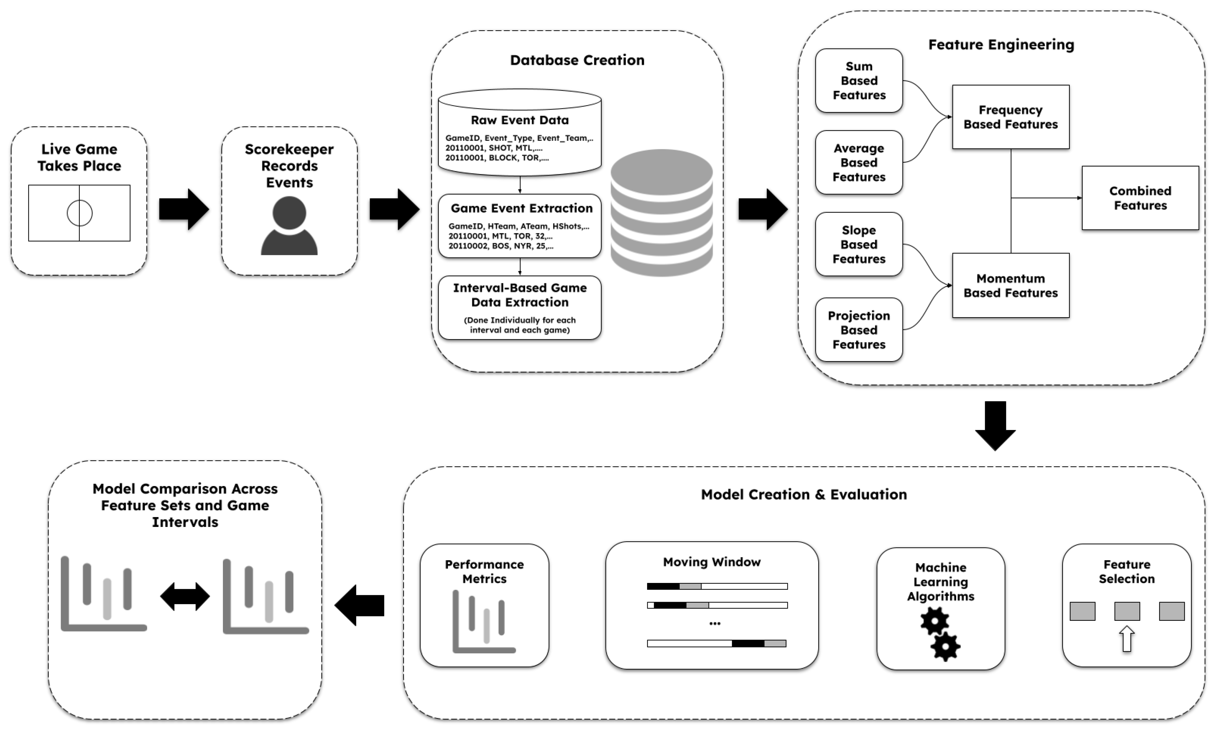
Figure 1 outlines the data pipeline proposed in this paper. Our pipeline starts with a raw dataset that includes individual events over games we intend to characterize. We then summarize individual games in our game event extraction, which groups events to determine key performance indicators in a game. We create the distinct features of our frequency-based, momentum-based, and combined feature sets using our game events. These feature sets are then fed into machine learning algorithms. The performance of these models is then evaluated with chosen performance metrics. Afterwards, the models are compared to each other, aiming to determine which groups of features have more predicting power.

3.1. Data Sources

The NHL dataset was sourced from a Python module called Hockey Scraper created by Harry Shomer5. This module scraped all NHL event data from the NHL’s public API for 2011 to 2020. For this dataset, we only included games that ended in the regular time frame. Overtime games are often close and do not help models distinguish between the binary targets of a home win or away win. We also removed each team’s first 20 games from each season, as they seem to struggle with consistency up to this point in the season. Both of these steps are often used in the training set for NHL pre-game prediction models, and we were inspired to do this by the work done by Peter Tanner on MoneyPuck.com6. We combined the scraped event data with expected goals data, also sourced from MoneyPuck.com, to ensure we had a solid dataset to build our models upon.

The NBA dataset was sourced from Kaggle7. This dataset held all play-by-play data for the NBA from 2015 to 2020. The NBA has a similar format to the NHL; each team plays 82 games a season, and ties after regulation are settled through overtime. We also found that removing overtime games and each team’s first 20 games yielded similar results, and therefore, we performed these steps as we did for the NHL dataset.

The European football/soccer dataset came from the public dataset released by Pappalardo et al. [21] using data collected by Wyscout. This dataset contained data from only the 2017 season; however, it contained these data for each of the five major first-division European leagues, those leagues being the first division in Spain, Italy, England, Germany, and France. We could view the data from these five competitions as five seasons of data. Due to the fact these leagues do not include overtime periods, we did not have to remove any games for that purpose. However, we removed each team’s first seven games, as the number of games per team per season in the five major leagues ranges from 34 to 38. This is nearly the same percentage of games removed per season from the NHL and NBA datasets.

3.2. Game Event Extraction

Using the raw data as our main source, we created individual game events that captured all the main events in a given game. This was done by grouping events based on their unique game ID. Each dataset had its way of uniquely identifying games. The NHL uniquely identified games with pairs of game IDs and the season in which the game took place. The Soccer dataset took the same approach, while the NBA dataset used the home team, away team, and date to identify each game.

We created a unique game ID for each game so that we would only require a single column to uniquely identify a game. We combined the season and game ID strings for the NHL and Soccer datasets to create a single game ID string. This works as follows. If the game had the ID “1115” and was being played in the 2015 season, our created game ID would be “20151115”. In the NBA, we used the season and a counter variable that incremented each new game. For example, the first game of the 2015 season would be game ID “201500001”, and the second game would be “201500002”, and so on.

These unique game IDs allowed us to create the game events by querying the raw datasets. For example, if we were looking to determine the number of shots the home team took in a given game, we would count the number of “SHOT” events that contained the unique game ID in the game_id column and contained the home team in the event_team column. This allowed us to summarize the outcome of each game from the event data and discern statistics such as the score, number of shots, shooting percentage, and more.

Table 1. Example of the data contained in each game event for the NHL.

Game ID	Away Team	Home Team	Away Goals	Home Goals	Away Shots	…
20150001	MTL	TOR	3	2	25	…
20150002	CAL	EDM	1	3	30	…
20150003	MIN	PIT	2	0	22	…
…	…	…	…	…	…	…

displays a small amount of the information that is held in each game event and shows how they are organized in the database.

3.3. Interval-Based Game Data Extraction

One of the fundamental parts of our pipeline is the game intervals. These intervals represent the number of games used to assess team quality in our models. For each game in our dataset, we would use the previous n games to gather statistics representing each team’s quality. For example, if we use an interval of three games, we will only use each team’s last three games when creating the features that represent the quality of those teams for a given game we are trying to predict the outcome of. Specifically, this paper uses intervals of 3 to 10 games.

For each game and each game interval, this extraction must take place. The data from interval-based extraction are used to calculate the values for our features and are, therefore, calculated concurrently with our feature set extraction to ensure that only one extraction of interval-based data takes place, thereby making the parsing of the data more computationally efficient.

The game IDs that were previously discussed can help improve this process. If IDs are sequential, that is, the IDs increase in the order of game occurrence, we can extract the n most recent games by getting all games involving a given team that has a game ID less than the ID of the game we are modeling; from there, we get the n games with the highest game ID. If the game IDs are not sequential, a better approach would be to retrieve the most recent games using their dates.

3.4. Feature Engineering

This work considers three feature sets in our pipeline: frequency-based, momentum-based, and combined. The frequency-based and momentum-based features have different sub-features, which we will discuss below. The combined feature set represents the combination of both the frequency-based and momentum-based feature sets. The features that were used by the models can be seen in

Table A1. The statistics that were used to create the features for the NHL model.

Statistic	Sum-Based	Average-Based	Slope-Based	Projection-Based
Wins	✓
Losses	✓
Goals For	✓	✓	✓	✓
Goals Against	✓	✓	✓	✓
Goals For 5v5	✓	✓	✓	✓
Goals Against 5v5	✓	✓	✓	✓
Goals For 5v5 Close	✓	✓	✓	✓
Goals Against 5v5 Close	✓	✓	✓	✓
Shots For	✓	✓	✓	✓
Shots Against	✓	✓	✓	✓
CORSI	✓	✓	✓	✓
CORSI 5v5	✓	✓	✓	✓
CORSI 5v5 Close	✓	✓	✓	✓
Faceoffs	✓	✓	✓	✓
Hits For	✓	✓	✓	✓
Hits Against	✓	✓	✓	✓
Penalty Minutes For	✓	✓	✓	✓
Penalty Minutes Against	✓	✓	✓	✓
Blocks For	✓	✓	✓	✓
Blocks Against	✓	✓	✓	✓
Giveaways For	✓	✓	✓	✓
Giveaways Against	✓	✓	✓	✓
Takeaways For	✓	✓	✓	✓
Takeaways Against	✓	✓	✓	✓
xG For	✓	✓	✓	✓
xG Against	✓	✓	✓	✓
xG For 5v5	✓	✓	✓	✓
xG Against 5v5	✓	✓	✓	✓
xG For 5v5 Close	✓	✓	✓	✓
xG Against 5v5 Close	✓	✓	✓	✓
Power Play Opportunities For	✓	✓	✓	✓
Power Play Opportunities Against	✓	✓	✓	✓
Power Play Goals For	✓	✓	✓	✓
Power Play Goals Against	✓	✓	✓	✓

,

Table A2. The statistics that were used to create the features for the NBA model.

Statistic	Sum-Based	Average-Based	Slope-Based	Projection-Based
Wins	✓
Losses	✓
Points For	✓	✓	✓	✓
Points Against	✓	✓	✓	✓
Field Goal Percentage For	✓	✓	✓	✓
Field Goal Percentage Against	✓	✓	✓	✓
Free Throw Percentage For	✓	✓	✓	✓
Free Throw Percentage Against	✓	✓	✓	✓
3-Point Field Goal Percentage For	✓	✓	✓	✓
3-Point Field Goal Percentage Against	✓	✓	✓	✓
Rebounds For	✓	✓	✓	✓
Rebounds Against	✓	✓	✓	✓
Offensive Rebounds For	✓	✓	✓	✓
Offensive Rebound Percentage For	✓	✓	✓	✓
Offensive Rebounds Against	✓	✓	✓	✓
Offensive Rebound Percentage Against	✓	✓	✓	✓
Defensive Rebounds For	✓	✓	✓	✓
Defensive Rebound Percentage For	✓	✓	✓	✓
Defensive Rebounds Against	✓	✓	✓	✓
Defensive Rebound Percentage Against	✓	✓	✓	✓
Assists For	✓	✓	✓	✓
Assists Against	✓	✓	✓	✓
Steals For	✓	✓	✓	✓
Steals Against	✓	✓	✓	✓
Blocks For	✓	✓	✓	✓
Blocks Against	✓	✓	✓	✓
Turnovers For	✓	✓	✓	✓
Turnovers Against	✓	✓	✓	✓
Effective Field Goal Percentage For	✓	✓	✓	✓
Effective Field Goal Percentage Against	✓	✓	✓	✓
True Shooting Percentage For	✓	✓	✓	✓
True Shooting Percentage Against	✓	✓	✓	✓

and

Table A3. The statistics that were used to create the features for the European football/soccer model.

Statistic	Sum-Based	Average-Based	Slope-Based	Projection-Based
Wins	✓
Losses	✓
Draws	✓
Goals For	✓	✓	✓	✓
Goals Against	✓	✓	✓	✓
Shots For	✓	✓	✓	✓
Shots Against	✓	✓	✓	✓
Shots On Target For	✓	✓	✓	✓
Shots On Target Against	✓	✓	✓	✓
Corners For	✓	✓	✓	✓
Corners Against	✓	✓	✓	✓
Corners On Target For	✓	✓	✓	✓
Corners On Target Against	✓	✓	✓	✓
Fouls For	✓	✓	✓	✓
Fouls Against	✓	✓	✓	✓
Yellow Cards For	✓	✓	✓	✓
Yellow Cards Against	✓	✓	✓	✓
Red Cards For	✓	✓	✓	✓
Red Cards Against	✓	✓	✓	✓
Passes For	✓	✓	✓	✓
Passes Against	✓	✓	✓	✓
Passes On Target For	✓	✓	✓	✓
Passes On Target Against	✓	✓	✓	✓
Free-kicks For	✓	✓	✓	✓
Free-kicks Against	✓	✓	✓	✓
Free-kicks On Target For	✓	✓	✓	✓
Free-kicks On Target Against	✓	✓	✓	✓

. The features extracted from the data are largely reflections of the event types recorded in each dataset. However, in the case of the NHL and NBA, more advanced performance indicators were extrapolated using the data. The advanced metrics used from each of these datasets were influenced by performance indicators discussed in other research, such as work in ice hockey by Johansson, Wilderoth, and Sattari [22] and work in basketball by Kubatko, Oliver, Pelton, and Rosenbaum [23]. Some popular public sources were also consulted, such as Natural Stat Trick8 and Basketball-Reference9.

3.4.1. Frequency-Based

Two separate frequency-based feature types are considered in our pipeline, named sum-based and average-based features. These features represent a primarily static and traditional approach to pre-game prediction in sports. These features are created by first querying data from each team’s previous n games as defined by our game interval. From there, we select a statistic for which we are creating these features, such as shots or blocks. Lastly, we extract features from the chosen statistic. Sum-based features are the sum of the statistics over the previous n games as defined by the game interval, i.e., the total number of shots over the last three games. At the same time, average-based features are the average statistical value achieved over the previous n games, i.e., the average number of shots over the last three games.

Table 2. Example of statistics over a team’s last three games.

Game Date	Number of Shots	Number of Goals
1 January	25	0
3 January	42	3
6 January	35	4
7 January	?	?

shows statistics achieved by a given team over the last three games. The question marks represent values for the game we are looking to predict. We use this table to illustrate how to create sum-based and average-based features to predict the outcome of the team’s upcoming game on 7 January. If we were to calculate the sum-based feature for the shots statistic on this set of recent games, we would add 25, 42, and 35 together, giving us a sum-based shot feature of 102. If we were now to calculate the average-based goal feature, we would divide the total number of goals by the number of games in the interval. So, we would divide 7 by 3, giving us an average-based goal feature of 2.33.

3.4.2. Momentum-Based

This work defines two separate momentum-based feature types: slope-based and projection-based. Slope-based features are created as follows: first, we query data from each team’s previous n games. We then select a statistic, such as shots, blocks, goals, etc., to create momentum-based features. Using the queried data from the recent games and our selected statistic, we create a two-dimensional space to plot our data, where the x-axis represents the passing of days between games, and the y-axis represents the statistical value they obtained for each given game. For example, if we had chosen the number of shots for our statistic, we would have plotted the number of shots for each game on the y-axis, with the x-axis representing the passing of days between games starting at $x=0$ for the first/earliest game in the interval. With these points, we calculate the linear line of best fit, and the slope of such a line would be our slope-based feature. Projection-based features are essentially just an extension of our slope-based features. Using the equation of the line of the best fit, we calculate the slope-based feature. We add the x value, which is the number of days that have passed since the first day in our game interval, and we project the statistical value for the upcoming game if the given trends continue.

We feel that an example can best show how these features are calculated. Suppose we are trying to calculate the slope-based and projection-based features using a three-game interval for the team in Table 2. We have chosen the number of shots to be the statistic we are using for our calculations, and we are calculating features for the upcoming game on 7 January. Using these data, we plot the data in the two-dimensional space as previously stated. Starting with the first game in our interval, which is the game on 1 January, we would plot $x=0$, $y=25$. From there, we would count the days between the game on the 1st and the 3rd; there are two days between these games, so next, we would plot $x=2$, $y=42$. Lastly, we would note that 6 January is five days after 1 January, so we plot $x=5$, $y=35$. With the points we have plotted, we can calculate the linear line of best fit; this line of best fit is represented by the equation $y=1.657x+30.13$. From this equation, we can see that our slope-based feature would be 1.657. Now, using the line of best fit, we can calculate our projection-based feature. Using the fact that 7 January is six days after our first game in the interval on 1 January, we plug $x=6$ into our previously stated line of best-fit equation. This gives us roughly $40.08$, which would be our projection-based feature and represents how many shots the team should have if recent trends continue. This example can be seen in Figure 2.

3.5. Model Evaluation/Comparison

We use a moving window to generate the data folds rather than evaluating our models using a standard cross-validation approach. This is because sports events are, in many ways, temporal data, and therefore, we do not want future events to be predicting past events. While this approach may slightly decrease our predictive power because we will be training on significantly fewer games than we would when using a traditional 80:20 split and cross-validation, we believe it maintains the integrity of the temporal data.

Our moving window first sorts all games in order of their occurrence. From there, we determine the number of games the model should train on and the number of games it should test on; these numbers are different for each sport we will discuss. Next, we divide all games into 20 equal train-test splits, such that a model is trained on a group of games and then tested on a group of games that begin immediately after the last game in the training set, thus ensuring that the future is not predicting the past. Therefore, these train-test splits move from left to right in the window of time.

As we alluded to, the train-test size is different for each sport due to the difference between the number of games in a season for each sport. The training and testing windows in the NHL and NBA are the same size, as teams in both leagues have 82-game seasons. The training and testing size used for the NHL/NBA is 2460 and 1230, respectively. We need to use much smaller training and testing sizes in the soccer dataset, as teams play significantly fewer games, with only 34 to 38 games for each team in a given season and fewer teams playing in the league. The training and testing sizes used for the soccer dataset are 760 and 380, respectively. These sizes were chosen to represent roughly two seasons of training and one season of testing in all three sports.

We adjusted the feature representation before our data were fed into our machine learning algorithms. Rather than having two values for each feature, one for the home team and one for the away team, we created one singular feature by subtracting the away feature from the home feature. For example, if we were creating our goals feature, and the value for the home team was 10 while the value for the away team was 7, we would subtract 7 from 10, giving us 3 for our goals feature. Our inspiration for this type of feature representation came from the work of Pischedda [15], who found that this increased the predictive power of their NHL game prediction model. We came to the same conclusion when testing our models and using this feature representation.

We have included feature selection approaches in our pipeline. We tested multiple approaches, such as recursive feature selection and sequential feature selection. However, we obtained the best results with the SelectBestK method. This method is handed some features to select (k) as a parameter and then selects the k best-scoring features from the complete feature set for a chosen statistical measurement. We used this method to select the best half of the available features for each model per their scoring based on mutual information. We perform feature selection on each training set in the moving window. This means we perform it 20 separate times, once for each training and testing set, which can result in slightly different features being chosen each time. We chose to do this because selecting features based on the entire dataset may introduce a bias into our moving window that unfairly increases the performance of our models.

We used three separate machine learning approaches for our models: logistic regression, random forest [24], and linear discriminant analysis (LDA). While we attempted to use more powerful techniques such as XGBoost [25] and neural networks, all gradient boosting methods yielded inferior results with our data. When testing neural networks, we found it was impossible to produce a neural network that was not biased toward one feature set or the other, and the logistics of having a network for each model and feature set was beyond the scope of what we are proposing here, as our focus is the data pipeline itself. However, we should note that any machine learning techniques could be employed in this pipeline.

To evaluate our models’ predictive power, we used the accuracy metric from Sklearn [26]. After our models have predicted the outcome of each game in the testing set, the accuracy metric determines what percentage of those predictions were correct. Our data manipulation and model evaluation were done using the Python programming language. For our data manipulation, we relied heavily on the Pandas module [27], while our machine learning algorithms and evaluation metrics were all imported through Sklearn [26]. Lastly, we created data visualizations that show the average accuracy obtained at each game interval for each machine learning technique and each sport. These visualizations were created using the Matplotlib and Seaborn modules [28,29].

We should also note the hyperparameters used with our machine learning techniques. Logistic regression used all default hyperparameters, except for max iterations set to 10,000. Random forest used a random state of 1415 to ensure reproducibility and had the number of estimators set to 20% of the training window size. Lastly, LDA used all default hyperparameters as well.

4. Results

Below, we present the results obtained from each machine learning technique we employed. In all figures of this subsection, we report the average accuracy of the 20 equal train-test splits in the NHL, NBA, and football/soccer datasets. In Section 4.1, we show the results obtained when using logistic regression, followed by Section 4.2, which shows the results obtained when using random forest. Lastly, Section 4.3 shows the results obtained when using LDA.

4.1. Logistic Regression

In Figure 3 and

Table 3. Average accuracy obtained from the 20 train-test splits of the moving window for each league and feature set when using logistic regression. The highest average accuracy for each league at each game interval is represented in bold font.

League	Feature Set	Interval of Games Used
		3	4	5	6	7	8	9	10
	Frequency	0.5535	0.5594	0.5623	0.5669	0.5743	0.5824	0.5889	0.5916
NHL	Momentum	0.5612	0.5606	0.5682	0.5691	0.5645	0.5760	0.5661	0.5720
	Combined	0.5504	0.5608	0.5580	0.5653	0.5738	0.5763	0.5819	0.5802
	Frequency	0.6051	0.6199	0.6310	0.6411	0.6442	0.6387	0.6479	0.6451
NBA	Momentum	0.5742	0.5821	0.5939	0.5858	0.6008	0.6039	0.6035	0.6066
	Combined	0.6044	0.6287	0.6346	0.6333	0.6422	0.6318	0.6411	0.6445
	Frequency	0.6434	0.6538	0.6457	0.6481	0.6423	0.6484	0.6433	0.6628
Soccer/Football	Momentum	0.6165	0.6230	0.6448	0.6509	0.6480	0.6477	0.6293	0.6459
	Combined	0.6468	0.6417	0.6394	0.6475	0.6324	0.6341	0.6328	0.6430

, our logistic regression analysis reveals intriguing findings. It becomes evident that the performance of various feature sets differs across different sports leagues. In the NHL, for instance, the momentum-based models exhibit superior performance when game intervals are shorter. In contrast, frequency-based features and combined features consistently outperform momentum-based features for the NBA across all game interval durations. Turning our attention to soccer, we observe that the momentum-based model excels when game intervals range from six to seven, while frequency-based and combined features perform similarly to each other throughout all intervals. Logistic regression consistently delivers the highest average accuracy across all three sports, underscoring its effectiveness in our analysis.

4.2. Random Forest

In Figure 4 and

Table 4. Average accuracy obtained from the 20 train-test splits of the moving window for each league and feature set when using random forest. The highest average accuracy for each league at each game interval is represented in bold font.

League	Feature Set	Interval of Games Used
		3	4	5	6	7	8	9	10
	Frequency	0.5414	0.5459	0.5473	0.5505	0.5582	0.5656	0.5643	0.5647
NHL	Momentum	0.5419	0.5431	0.5455	0.5561	0.5436	0.5502	0.5511	0.5466
	Combined	0.5536	0.5578	0.5566	0.5645	0.5618	0.5671	0.5707	0.5692
	Frequency	0.5829	0.5916	0.5971	0.6074	0.6234	0.6267	0.6248	0.6282
NBA	Momentum	0.5530	0.5641	0.5754	0.5805	0.5752	0.5952	0.5855	0.5992
	Combined	0.5802	0.5901	0.6030	0.6069	0.6193	0.6185	0.6208	0.6291
	Frequency	0.6328	0.6250	0.6385	0.6263	0.6393	0.6360	0.6372	0.6325
Soccer/Football	Momentum	0.5663	0.5808	0.6056	0.6145	0.6184	0.6224	0.6208	0.6274
	Combined	0.6316	0.6272	0.6410	0.6381	0.6353	0.6408	0.6339	0.6458

, some interesting observations emerge as we present the results obtained for the random forest model. Momentum-based models, it appears, do not exhibit strong performance across any of the sports. In contrast, the combined and frequency-based feature sets consistently yield better results across all three sports. Notably, in both the NHL and soccer datasets, the combined features display an edge over the frequency-based feature set, suggesting that combining frequency-based and momentum-based features may offer a promising approach to enhance prediction accuracy. This can also be seen to a lesser extent in the NBA.

4.3. Linear Discriminant Analysis

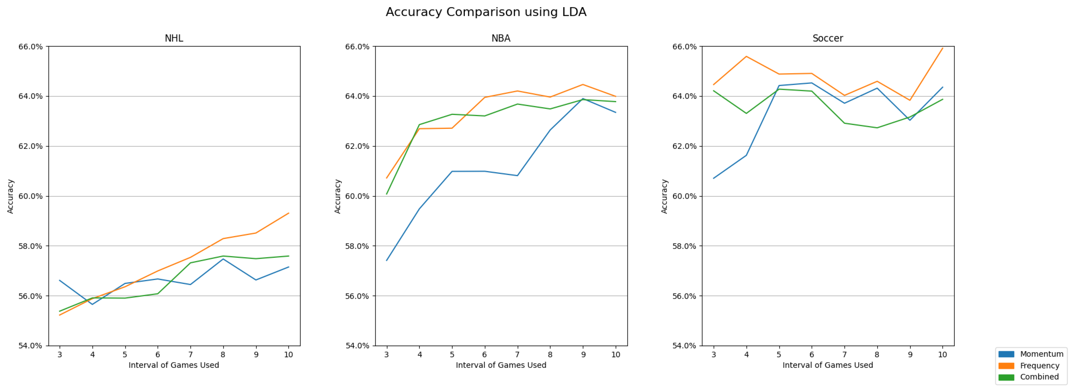
Utilizing linear discriminant analysis (LDA) reveals a consistent preference for the frequency-based feature set, a trend evident in Figure 5 and

Table 5. Average accuracy obtained from the 20 train-test splits of the moving window for each league and feature set when using LDA. The highest average accuracy for each league at each game interval is represented in bold font.

League	Feature Set	Interval of Games Used
		3	4	5	6	7	8	9	10
	Frequency	0.5522	0.5588	0.5636	0.5699	0.5753	0.5829	0.5851	0.5931
NHL	Momentum	0.5661	0.5565	0.5649	0.5667	0.5645	0.5747	0.5663	0.5715
	Combined	0.5538	0.5591	0.5590	0.5608	0.5732	0.5759	0.5748	0.5759
	Frequency	0.6071	0.6269	0.6271	0.6394	0.6415	0.6396	0.6446	0.6398
NBA	Momentum	0.5741	0.5948	0.6098	0.6098	0.6081	0.6264	0.6390	0.6334
	Combined	0.6007	0.6285	0.6327	0.6320	0.6368	0.6348	0.6385	0.6377
	Frequency	0.6446	0.6559	0.6488	0.6490	0.6402	0.6459	0.6383	0.6591
Soccer/Football	Momentum	0.6070	0.6162	0.6442	0.6452	0.6371	0.6431	0.6303	0.6435
	Combined	0.6421	0.6330	0.6427	0.6419	0.6291	0.6272	0.6316	0.6387

. However, a couple of notable results are present. The NHL dataset mirrors the initial advantage for momentum-based features observed with short game intervals when using logistic regression. We consistently observe a preference for frequency-based features in the NBA dataset across all but two game intervals. In the soccer dataset, the frequency-based features excel at all intervals. However, all feature sets seem to perform well in the soccer dataset.

5. Discussion

Upon examining our results, several compelling patterns come to light. Notably, in the context of the NHL dataset, we discern potential evidence of momentum’s influence across all three machine learning techniques employed. Both logistic regression and LDA reveal that momentum-based features and, at times, combined features hold an early predictive advantage over the frequency-based feature set. This finding carries notable significance, suggesting that a team’s performance trend, as opposed to their aggregated and averaged performance over the same period, better predicts outcomes when we only consider a small sample of recent games to access team quality. This insight implies that momentum can wield predictive power, particularly for outcomes over shorter spans of games such as three or four. It is essential to clarify that this does not imply that momentum-based features or momentum itself are universally superior predictors; instead, it underscores that momentum-based features can enhance more intricate models by offering valuable insights into short-term performance.

In the case of random forest and the NHL dataset, we observe that a combination of momentum-based and frequency-based features exhibits the highest predictive efficacy. Given that random forest is a more powerful technique than logistic regression and LDA, this outcome suggests that the model places significant weight on specific features from the combined feature set. This finding emphasizes the potential advantages of employing combined features when the goal is to predict the game outcome, provided that feature selection and hyperparameter tuning are rigorously performed, particularly in the context of more complex machine learning techniques.

In the NBA dataset, our analysis reveals a minimal effect attributable to momentum across all three machine learning approaches applied in this study. At times, we see advantages when using the combination of both frequency-based and momentum-based features, but these advantages are rare and short-lived. Several factors may contribute to this lack of evidence, including the specific features we utilized, the level of hyperparameter tuning, or the inherent characteristics of the NBA itself. It is worth acknowledging that the NBA, as shown by Rockerbie [30], may exhibit distinctive attributes, such as lesser degrees of team parity and randomness, which can potentially impact the predictability of outcomes.

When examining the outcomes derived from our European football/soccer dataset, we uncover a particularly intriguing trend, mainly when focusing on the performance of momentum-based features, and notably within the context of logistic regression. In contrast to the NHL, where momentum-based features demonstrate an advantage over shorter intervals of three or four games, the soccer dataset presents a distinctive pattern. Here, the initial performance of momentum-based predictors is underwhelming, but they exhibit exponential growth in predictive power, reaching their peak at game intervals of six to eight. Notably, logistic regression showcases an accuracy peak at an interval of six to seven games. We also see the combined feature sets outperform the other feature sets the majority of the time when using random forest. Although the margins of this advantage are small, this recurring trend emphasizes the potential benefits of leveraging combined feature sets with more sophisticated machine learning techniques.

The primary objective of this study was to demonstrate the feasibility of comparing momentum’s impact within a given sport by utilizing both frequency-based and momentum-based features. We contend that we have effectively elucidated and substantiated the rationale behind this methodology. Furthermore, we have illustrated this approach’s practical implementation by contrasting momentum’s effects across three distinct datasets.

The outcomes presented in this study strongly suggest that team-based momentum is a tangible phenomenon, quantifiable through the use of momentum-based features. We believe these findings lay the foundation for future predictive models, which could employ a combined feature approach to capture short-term and long-term success in sports analytics more comprehensively.

On a more practical level, this work helps us differentiate the level to which momentum affects different sports, thus allowing us to contextualize other literature on the topic in their respective sports. For instance, studies that find no evidence of momentum in the NBA are no surprise, given our findings here. This work could also be adapted to examine how momentum affects individual teams differently. This, in theory, could give teams a better understanding of how an upcoming opponent may perform, given their predisposition to being affected by momentum or the lack thereof. For instance, if a team seems to be heavily affected by momentum, their upcoming opponents can put extra emphasis on their more recent games to judge the quality of the team.

In this work, we did not use neural networks due to the large scope of constructing multiple network architectures for each sport and feature set. However, we would like to explore how neural networks, particularly Long Short-Term Memories (LSTMs), interact with each feature set in future works. LSTMs are particularly interesting due to their advantages when using temporal data such as the datasets we have outlined in this manuscript. Ideally, we would like to construct a pipeline capable of engineering unique networks for each sport and feature set, thus allowing us to further our understanding of the predictive power of momentum-based features.

It is essential to acknowledge certain limitations in our overall approach. Our models did not implement a rigorous feature selection technique, nor a hyperparameter selection technique of any kind, potentially introducing bias towards specific feature sets in certain sports. In future research, a practical strategy that combines momentum-based and frequency-based features from various game interval durations may prove instrumental in achieving more accurate predictive models, particularly in sports like the NHL, where momentum exhibits more substantial indications. Additionally, our approach to engineering momentum-based features has two potential drawbacks. The first is related to cases where we use as few as three games for our game interval. In such instances, the residuals may deviate significantly from the line of best fit. Currently, there is no immediate solution to this issue in our research. Nevertheless, in future endeavors, exploring the possibility of exclusively predicting games for which the line of best fit results in an acceptable value for the residual sum of squares (RSS) may be worthwhile. Another essential concern is using momentum-based features with many recent games, such as 20 or more. In such cases, it is possible that the slope of the momentum-based feature could approach zero. However, employing a more significant number of games may not align with the conventional concept of momentum, which is typically viewed as a short-term phenomenon. As the slope feature approaches zero, it could be harnessed with the residual sum of squares (RSS) to gauge consistency in scenarios where larger game intervals are applied. Recognizing that these larger game intervals might also lead the projection-based feature to yield outcomes connected to those obtained through the average-based feature is essential. To avoid this, we recommend limiting the use of this method to no more than 10 to 12 recent games unless the objective is to measure consistency rather than momentum. The specific limit could vary, depending on the league’s structure for which predictions are made. It is crucial to clarify that our intention is not to imply that momentum-based features, in isolation, are inherently superior to frequency-based features. Instead, we aim to illustrate the ability to measure momentum in ways that extend beyond solely relying on sequential outcomes. Through these diverse approaches, we can gain insights into how momentum can influence different sports in distinctive manners, potentially paving the way for developing more robust pre-game prediction models.

6. Conclusions

In this work, we aimed to outline a data pipeline that could effectively compare and demonstrate the predictive power of momentum-based features among multiple sports leagues. We believe we have achieved that, and in its current state, this pipeline can be used to measure the effects of momentum in any sport for which event data are available and could also be adapted to view the effects of momentum on individual players. We also believe we have provided further insight into momentum by approaching the phenomenon from a trend-of-play perspective; we believe this view allows us to emphasize that momentum can be separate from game outcomes and that it is more important to focus on what historically leads to winning rather than winning itself. In the future, we would like to explore potential refinements to the pipeline to select the optimal features and hyperparameters for each model in order to explore the capabilities of the momentum-based features further, particularly when they are being combined with frequency-based features in more robust models such as random forest.

References

- Lewis, M. Moneyball: The Art of Winning an Unfair Game; WW Norton & Company: Manhattan, NY, USA, 2004. [Google Scholar]
- Miller, J.B.; Sanjurjo, A. A visible (hot) hand? Expert players bet on the hot hand and win. SSNR Elsevier 2017. [Google Scholar] [CrossRef]
- Vergin, R.C. Winning Streaks in Sports and the Misperception of Momentum. J. Sport Behav. 2000, 23, 181. [Google Scholar]
- Gilovich, T.; Vallone, R.; Tversky, A. The hot hand in basketball: On the misperception of random sequences. Cogn. Psychol. 1985, 17, 295–314. [Google Scholar] [CrossRef]
- Ritzwoller, D.M.; Romano, J.P. Uncertainty in the hot hand fallacy: Detecting streaky alternatives to random Bernoulli sequences. Rev. Econ. Stud. 2022, 89, 976–1007. [Google Scholar] [CrossRef]
- Miller, J.B.; Sanjurjo, A. Surprised by the hot hand fallacy? A truth in the law of small numbers. Econometrica 2018, 86, 2019–2047. [Google Scholar] [CrossRef]
- Arkes, J.; Martinez, J. Finally, evidence for a momentum effect in the NBA. J. Quant. Anal. Sport. 2011, 7, 1–16. [Google Scholar] [CrossRef]
- Fry, M.J.; Shukairy, F.A. Searching for momentum in the NFL. J. Quant. Anal. Sport. 2012, 8. [Google Scholar] [CrossRef]
- Taylor, J.; Demick, A. A multidimensional model of momentum in sports. J. Appl. Sport Psychol. 1994, 6, 51–70. [Google Scholar] [CrossRef]
- Leung, C.K.; Joseph, K.W. Sports data mining: Predicting results for the college football games. Procedia Comput. Sci. 2014, 35, 710–719. [Google Scholar] [CrossRef]
- Wang, Z.; Long, C.; Cong, G. Similar sports play retrieval with deep reinforcement learning. IEEE Trans. Knowl. Data Eng. 2021, 35, 4253–4266. [Google Scholar] [CrossRef]
- Wongta, N.; Natwichai, J. Data Pipeline of Efficient Stream Data Ingestion for Game Analytics. In Proceedings of the Advances in Internet, Data & Web Technologies: The 11th International Conference on Emerging Internet, Data & Web Technologies (EIDWT-2023), Semarang, Indonesia, 23–25 February 2023; Springer: Berlin/Heidelberg, Germany, 2023; pp. 483–490. [Google Scholar]
- Wongta, N.; Natwichai, J. End-to-End Data Pipeline in Games for Real-Time Data Analytics. In Proceedings of the Advances in Internet, Data and Web Technologies: The 9th International Conference on Emerging Internet, Data & Web Technologies (EIDWT-2021), Chiang Mai, Thailand, 25–27 February 2021; Springer: Berlin/Heidelberg, Germany, 2021; pp. 269–275. [Google Scholar]
- Thabtah, F.; Zhang, L.; Abdelhamid, N. NBA game result prediction using feature analysis and machine learning. Ann. Data Sci. 2019, 6, 103–116. [Google Scholar] [CrossRef]
- Pischedda, G. Predicting NHL match outcomes with ML models. Int. J. Comput. Appl. 2014, 101. [Google Scholar] [CrossRef]
- Rodrigues, F.; Pinto, Â. Prediction of football match results with Machine Learning. Procedia Comput. Sci. 2022, 204, 463–470. [Google Scholar] [CrossRef]
- Koehler, J.J.; Conley, C.A. The “hot hand” myth in professional basketball. J. Sport Exerc. Psychol. 2003, 25, 253–259. [Google Scholar] [CrossRef]
- Green, B.; Zwiebel, J. The hot-hand fallacy: Cognitive mistakes or equilibrium adjustments? Evidence from major league baseball. Manag. Sci. 2018, 64, 5315–5348. [Google Scholar] [CrossRef]
- Lopez, M.J.; Matthews, G.J.; Baumer, B.S. How often does the best team win? A unified approach to understanding randomness in North American sport. Ann. Appl. Stat. 2018, 12, 2483–2516. [Google Scholar] [CrossRef]
- Wunderlich, F.; Seck, A.; Memmert, D. The influence of randomness on goals in football decreases over time. An empirical analysis of randomness involved in goal scoring in the English Premier League. J. Sport. Sci. 2021, 39, 2322–2337. [Google Scholar] [CrossRef]
- Pappalardo, L.; Cintia, P.; Rossi, A.; Massucco, E.; Ferragina, P.; Pedreschi, D.; Giannotti, F. A public data set of spatio-temporal match events in soccer competitions. Sci. Data 2019, 6, 236. [Google Scholar] [CrossRef]
- Johansson, U.; Wilderoth, E.; Sattari, A. How Analytics is Changing Ice Hockey. In Proceedings of the Linköping Hockey Analytics Conference, Linköping, Sweden, 6–8 June 2022; pp. 49–59. [Google Scholar]
- Kubatko, J.; Oliver, D.; Pelton, K.; Rosenbaum, D.T. A starting point for analyzing basketball statistics. J. Quant. Anal. Sport. 2007, 3, 1. [Google Scholar] [CrossRef]
- Ho, T.K. Random decision forests. In Proceedings of the 3rd International Conference on Document Analysis and Recognition, Montreal, QC, Canada, 14–16 August 1995; IEEE: Piscataway, NJ, USA, 1995; Volume 1, pp. 278–282. [Google Scholar]
- Chen, T.; Guestrin, C. Xgboost: A scalable tree boosting system. In Proceedings of the 22nd Acm Sigkdd International Conference on Knowledge Discovery and Data Mining, San Francisco, CA, USA, 13–17 August 2016; pp. 785–794. [Google Scholar]
- Pedregosa, F.; Varoquaux, G.; Gramfort, A.; Michel, V.; Thirion, B.; Grisel, O.; Blondel, M.; Prettenhofer, P.; Weiss, R.; Dubourg, V.; et al. Scikit-learn: Machine Learning in Python. J. Mach. Learn. Res. 2011, 12, 2825–2830. [Google Scholar]
- McKinney, W. Data structures for statistical computing in python. In Proceedings of the 9th Python in Science Conference, Austin, TX, USA, 28 June–3 July 2010; Volume 445, pp. 51–56. [Google Scholar]
- Hunter, J.D. Matplotlib: A 2D graphics environment. Comput. Sci. Eng. 2007, 9, 90–95. [Google Scholar] [CrossRef]
- Waskom, M.L. seaborn: Statistical data visualization. J. Open Source Softw. 2021, 6, 3021. [Google Scholar] [CrossRef]
- Rockerbie, D.W. Exploring interleague parity in North America: The NBA anomaly. J. Sport. Econ. 2016, 17, 286–301. [Google Scholar] [CrossRef]
Figure 1.
A diagram of our complete data pipeline.
Figure 2.
Example of how momentum-based features are calculated with the use of the data in Table 2.
Figure 3.
A comparison of the accuracy achieved among different sports and feature sets using logistic regression.
Figure 4.
A comparison of the accuracy achieved among different sports and feature sets when using random forest.
Figure 5.
A comparison of the accuracy achieved among different sports and feature sets when using linear discriminant analysis.