

Introduction to Reproducible Geospatial Analysis and Figures in R: A Tutorial Article

BEAGx, Faculty of Gembloux Agro-Bio Tech, University of Liège, 5030 Gembloux, Belgium
*
Author to whom correspondence should be addressed.
Data 2024, 9(4), 58; https://doi.org/10.3390/data9040058
Submission received: 23 March 2024
/
Revised: 10 April 2024
/
Accepted: 14 April 2024
/
Published: 20 April 2024
(This article belongs to the Topic Techniques and Science Exploitations for Earth Observation and Planetary Exploration)
Abstract
:The present article is intended to serve an educational purpose for data scientists and students who already have experience with the R language and which to start using it for geospatial analysis and map creation. The basic concepts of raster data, vector data, CRS and datum are first presented along with a basic workflow to conduct reproducible geospatial research in R. Examples of important types of maps (scatter, bubble, choropleth, hexbin and faceted) created from open-source environmental data are illustrated and their practical implementation in R is discussed. Through these examples, essential manipulations on geospatial vector data are demonstrated (reading, transforming CRS, creating geometries from scratch, buffer zones around existing geometries and intersections between geometries).
1. Introduction
The R language [1] is a popular open-source tool for data analysis and generation of figures for scientific communication [2,3]. The open and collaborative nature of R allows its wide and varied user community to continuously extend its capabilities through “packages” hosted in repositories (the main of which is the Comprehensive R Archive Network (CRAN), https://cran.r-project.org (accessed on 20 March 2024).
Through the years, literate programming capabilities (generation of documents from code script) have been added to R through several packages (namely knitr [4,5,6], RMarkdown [7,8,9], bookdown [10,11]) and, more recently, through the multi-language and multi-engine Quarto software (https://quarto.org/ (accessed on 20 March 2024)). Literate programming has raised an ever-growing interest in the scientific community for several years for two reasons. First, and most importantly, it drastically improves transparency and computational reproducibility of scientific research, which has been identified as a critical point undermining the reliability of the scientific literature reliability in many fields and disciplines, including Earth and environmental sciences [12,13]. An increasing number of journals require that the raw data and scripts for data analysis be submitted along with manuscripts, and some of them already accept submission in Rmarkdown format [14]. The second reason is that it allows scientists to conveniently combine data analysis, figure generation and manuscript preparation (with automatic management of editing aspects such as formatting, bibliography, cross references…) in one single and convenient tool. Plentiful resources can be relied on to learn about using R for literate programming (e.g., [7,8,10,15,16]).
Numerous packages also brought geospatial information system (GIS) capabilities to R, making it a mainstream tool for reproducible GIS analysis [17,18]. Two significant examples include terra [19] and sf [20], both relying on external popular libraries (such as S2 [21], GEOS [22], GDAL [23] and PROJ [24]). Many packages can be used to produce maps in R, from general-purpose ones (such as base [1] ggplot2 [25] extended with ggspatial [26]) to specialized ones (such as tmap [27], cartography [18], leaflet [28], ggmap [29], mapdeck [30] or mapview [31]).
The present article aims to present the basics of geospatial analysis, geospatial data manipulations and map types with example application using the R language. This tutorial article focuses on the package sf [20] for geospatial data manipulation and on the package ggplot2 [25] for generating maps. The full RMarkdown script and the datasets used to prepare this manuscript available in Supplementary Materials.
2. The Basics of GIS and Geospatial Analysis
2.1. Geospatial Data Types and Formats
Vector and raster data are two fundamental types of data structures used in GIS [32]. Vector data represent discrete entities (features) as points, lines, and polygons encoded through the coordinates of their vertices [32]. Vector data types are suitable for discrete measurements and complex geometries such as lines (e.g., rivers) and polygons (e.g., countries) [32]. Raster data represent spatial information as a grid of cells or pixels, where each cell holds a value representing a specific attribute or phenomenon [32]. They can be used to represent continuous data such as land cover acquired through teledetection (satellite and drone imagery).
Geospatial data can be stored in various file formats. Table 1 lists some commonly encountered GIS formats.
Vector data formats (such as shapefile, geopackage and geoJSON) can be read in R using sf :: st_read [20] whereas raster data such as geoTIFF can be read using raster :: raster [37]. In addition to these specialized formats, GIS data are also commonly found in .csv and .xlsx formats. These file formats can be read using utilis :: read.csv [1] and openxlsx :: read.xlsx [38], respectively, and then converted to objects of class sf using sf :: st_as_sf [20], specifying the columns to use as coordinates and the CRS. Further details on GIS file formats can be found in [39].
2.2. Coordinate Reference System(CRS)
A coordinate reference system (CRS) is a framework used to define the positions of objects on the Earth’s surface. It consists of a coordinate system, which defines how coordinates are represented, and a datum, which specifies the reference point, orientation, and scale of the coordinate system [32,40].
There are two types of CRS: geographic and projected. Geographic CRSs represent the Earth’s surface as an ellipsoidal surface (specified in the datum) and refer to positions and distances as angles [32,40]. Projected CRSs represent Earth’s surface projections of geographic CRS on a virtual cone, cylinder or plane at a given location in space, with a given orientation, etc. The projection can then be represented on a flat surface (e.g., paper or screen) by “unfolding” the cylinder or cone [32,40]. Projected CRSs represent positions and distances as Cartesian coordinates on that flat surface. Although more practical for representation and some computation (as distance units can be expressed in metres or feet), the projection process always induces distortion [32,40].
Coordinate reference systems can be identified in different ways. The most currently common ways are the EPSG (European Petroleum Survey Group) identifier and the more complete WKT2 (“well-known text”) defined by the Open Geospatial Consortium [33] and transposed in ISO 19162 [41]. Table 2 lists some common CRS. Most often, countries use a specific CRS for maximum accuracy.
2.3. Workflow
The first step of spatial analysis is to find the supporting data that are necessary to contextualize the data set of interest. These can be coasts and national/administrative borders locations, land use data, hydrographic data, demographic data, etc. Such data can be obtained from national and international geographic, demographic and statistical institutions (such as Eurostat and the Joint Research Center for the European Union) in formats such as .csv or shapefiles which are read in R using utils :: read.csv [1] and sf :: st_read [20], respectively. Useful data can also be imported directly through specific packages such as rnaturalearth [42] and rnaturalearthdata [43] (data from https://www.naturalearthdata.com/ (accessed on 20 March 2024)), giscoR [44] (data from the geospatial open data repository of the European commission (GISCO)), geodata [45] (data from various sources).
After some data manipulation (examples are provided through the examples in the next section, further examples can be found in chapter 5 of [40]), maps can be generated using various packages. The present tutorial relies on the popular ggplot2 package [25] relying on the “grammar of graphics” paradigm [46] according to which the different elements of the plot (axis, labels, geometries…) are added in “layers” that can be controlled independently of each other, allowing fine tuning. Using ggplot2 functions, each layer is separated with “+”. The function ggplot2::geom_sf [25] 1 is designed to handle data from objects of class sf. The function ggplot2::coord_sf [25] 2 is used to control the area displayed on the map with the xlim and ylim arguments (the value supplied is interpreted in the distance unit of the CRS). Finally, as their name suggests, the functions ggspatial :: annotation_scale and ggspatial :: annotation_north_arrow [26] are used to add a scale and an indication of direction, respectively. Finally, figures can be exported in common formats such as .png and .svg using ggplot2 :: ggsave [25].
3. Example of Common Map Types
3.1. Scatter Map
A scatter map is the simplest type of map used to represent data points on a map, usually with a color proportional to a given variable. In this first example, a scatter map representing the soil organic carbon (SOC) content measured across Germany (data from Poeplau et al. [49]) is prepared.
The data are first loaded from tidyr :: xlsx files using openxlsx :: read.xlsx [38] and stored as objects of class df. The mean SOC is calculated for each sampling location using dplyr :: group_by and dplyr :: summarise [50]. The measurement and sampling location data are merged using base :: merge [1]. The data are converted to an object of class sf using sf :: st_as_sf [20], specifying the columns to use as coordinates and the CRS.
The background map of the European Nomenclature of Territorial Units for Statistics (NUTS) is loaded using giscoR :: gisco_get_nuts [44]. This function allows us to download the map with three available CRS: EPSG 4326 (default), EPSG 4258, EPSG 3035 and EPSG 3857. Since the ESPG of the data is EPSG 25832, the CRS of either the data or the map must be changed to match the other. In the present example, the CRS of the map is changed because EPSG 25832 is more accurate for the region of interest. A dummy boolean variable is created to indicate whether the polygon belongs to Germany or not. This variable is used later to distinguish Germany from other countries on the maps.
![Data 09 00058 i001]()

When generating plots using ggplot2 [25], the default color scale fits the whole range of the data for the represented variable. In frequent cases (e.g., presence of outliers or highly skewed distribution), most data may fall within a narrow range of the color scale, making it rather uninformative. In the present example, this is overcome by scaling the minimum and maximum values of the scale to specific quantiles using the limits argument of viridis :: scale_color_viridis [51] and by adding the argument oob= scales :: squish [52] (which replaces out of bounds (oob) values with the closest limit). The viridis color scales have the advantage of remaining readable with color-blindness [51]. The axis range of the map is defined by supplying values from sf :: st_bbox [20] (which calculates a bounding box of its input) to ggplot2 :: coord_sf [25] to automatically “zoom” on the area of interest. The functions ggplot2 :: scale_fill_manual [25] and ggplot2 :: guides [25] are used to assign a distinct color to Germany and hide the legend for the associated dummy variable, respectively. The resulting map is shown in Figure 1.
![Data 09 00058 i002a]()
![Data 09 00058 i002b]()


In the following example, a map of the watercourses with a long-term average discharge higher than 10 m³/s in Germany along with a buffer zone of 20 km around them is generated to exemplify line geometries and buffer zones (the data are taken from the HydroRIVERS dataset [53]). First, the hydrographic data are read from a shapefile, the CRS of the data is transformed to the same CRS as the map and only watercourses with a flow higher than 10 m³/s are retained using dplyr :: filter [50]. Then, a buffer zone of 20 km around all watercourses is calculated using sf :: st_buffer [20]. Since a buffer is calculated for each line segment, all buffers are melted together using sf :: st_union [20]. The result is shown in Figure 2.
![Data 09 00058 i003]()

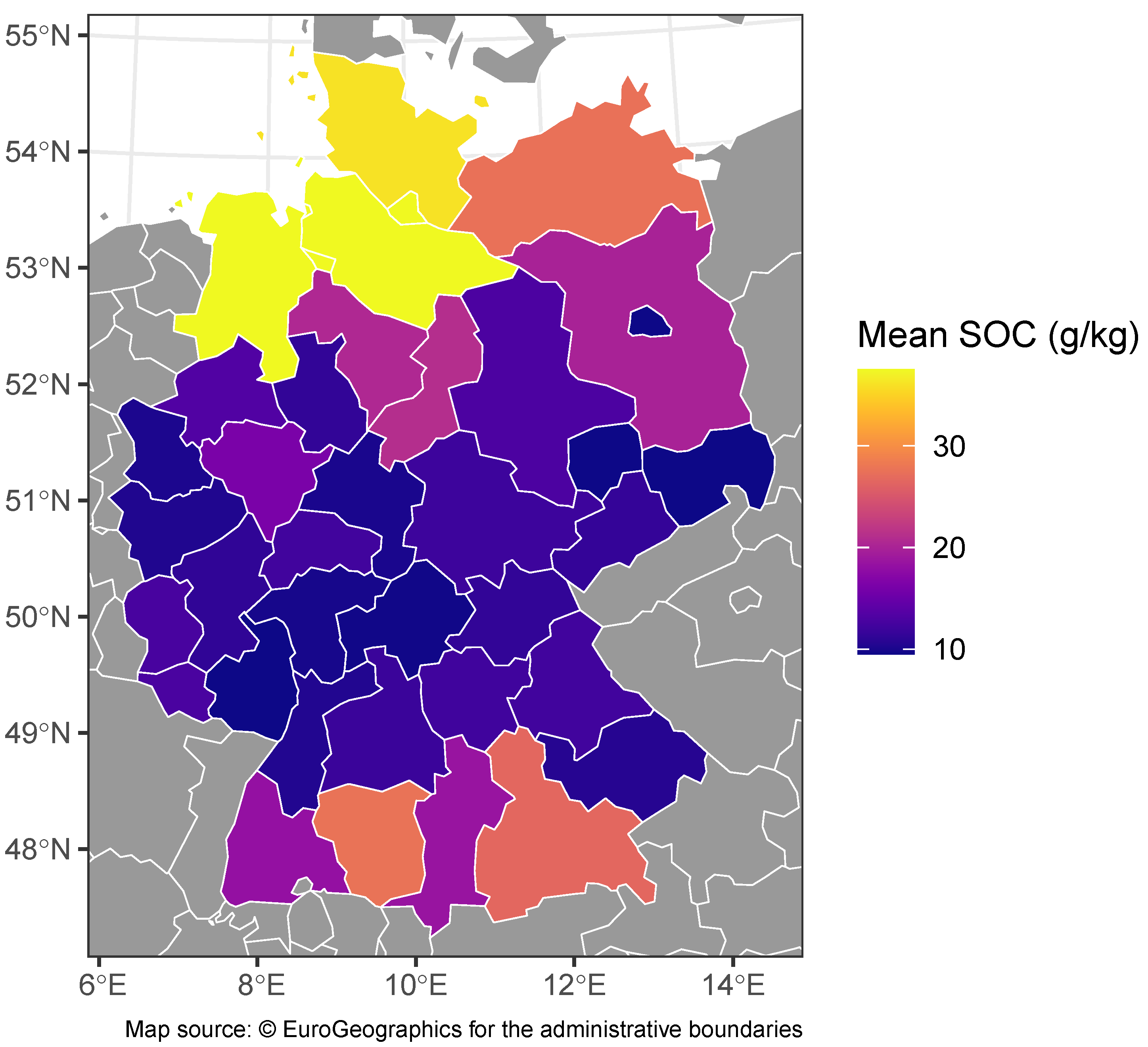
3.2. Choropleth Maps
A choropleth map is a type of map where arbitrary areas (usually administrative) are colored accordingly with a given variable (usually an aggregate statistic). Choropleth maps are most useful when the data are meaningful to the geographic segmentation (e.g., economic and demographic data such as per capita income, gross domestic product…).
In the example below, a choropleth map is used to represent the soil organic carbon (SOC) content measured across Germany. First, each point is associated with the NUTS in which it is located using sf :: st_intersection [20]. The mean for each NUTS is calculated and joined with the corresponding geometries. The geometries must be dropped from the means with sf :: st_drop_geometry [20] since sp :: merge can only join an object of class sf with an object of class df. The resulting choropleth map is shown in Figure 3.
![Data 09 00058 i004a]()
![Data 09 00058 i004b]()


3.3. Hexbin Map
Hexbins are the two-dimensional analogs of histograms with hexagon-shaped cells. Hexbin maps are somewhat in-between scatter maps and choropleth maps: they can be used to represent aggregate data over space, but unlike choropleth maps, the segmentation is regular and not related to a meaningful characteristic such as a national border. The relevance of the information communicated depends heavily on the granularity (i.e., cell size). Hexbins should only be used for relatively small areas (e.g., country or smaller), as the wider the area represented on a map, the more distorted the cells will be in the real space when applied to a planar projection.
Square counterparts also exist (“fishnets” maps). The process of generating a fishnet map can be assimilated into the conversion of vector data to raster data (“rasterization”) [40].
In the following example, the mean soil organic carbon (SOC) content measured across Germany is represented in a hexbin map. To achieve this, a hexagon grid covering the data is generated using sf :: st_make_grid [20] with the argument square = FALSE (this step is also called tesselation) and formatted into an object of class sf using sf :: st_sf [20]. The desired cell size is specified with the argument cellsize. The value for this argument must be supplied with a unit compatible with the unit specified in the CRS, which can be specified with units :: as_units [54]. It follows that it is not straightforward to set a cell size area when the unit of the CRS is degrees (which is the case for the widespread EPSG 4326).
Since ggplot2 :: coords_sf [25] displays an area slightly larger than the one specified using ggplot2 :: coord_sf [25], the tesselation is performed on an area expanded by a factor 0.25 compared to the area of interest covered by the data. The result is shown in Figure 5.
![Data 09 00058 i006a]()
![Data 09 00058 i006b]()


In the previous example, the grid was generated in such a way that hexagons have the same size on the projected map. Because of the projection, the actual area of the hexagons is not exactly identical. The broader the geographic area covered, the higher the deviation between cells.
Alternatively, it is possible to generate a grid with cells of actual regular size/area using the package dggridR. A dggr object representing the desired grid is obtained with dggridR:: dgconstruct [55]. The resolution parameter is selected from 0 to 30 (each resolution corresponds to a given division of Earth’s surface; the corresponding number of cells and area can be consulted by running dggridR:: dginfo [55]). Various grids are available. In the present example, the default grid (“ISEA3H”) is used.
The function dggridR:: dgrectgrid is then used to generate the grid as an object of class sf based on the dggr object and coordinates of the bounding box covering the area of interest in degree longitude/latitude. The following steps are identical to the first hexbin map example. The result is shown in Figure 6.
![Data 09 00058 i007a]()
![Data 09 00058 i007b]()


The main disadvantage of the dggridR approach is that the cell area must be selected among available ones.
3.4. Bubble Map
A bubble map is very similar to a scatter map, except that the sizes of the dots (or another shape) are proportional to a variable (instead or in addition to color).
In the following example, a bubble map is used to illustrate the mean concentration of particulate matter with an aerodynamic diameter smaller than 10 µm (PM10) across the United Kingdom in the period 2016–2019 (source data: [56,57]). Again, the data are read from tabular format (in this case, .csv) and converted to an object of class sf using sf :: st_as_sf [20]. Since the CRS is not specified, the default WGS84 (EPSG 4326) is assumed. To produce a more accurate map, the CRS is changed to the British National Grid (EPSG 27700), a more specific CRS for this region. The CRS of the map is also changed to match the CRS of the data.
For this example, the location data were deliberately converted to a simple feature before merging with the measurement data. When merging an object of class sf with an object of class df using sp :: merge [58], the first must be supplied to the x argument and the second to the y argument.
![Data 09 00058 i008]()

A single combined legend for multiple aesthetics (size and color) can be obtained by using ggplot2 :: guides and supplying ggplot2 :: guide_legend [25] to arguments of each aesthetic. The labels in the legend for both aesthetics (specified using ggplot2 :: labs [25]) must also be identical. The map obtained is displayed in Figure 7.
![Data 09 00058 i009a]()
![Data 09 00058 i009b]()


3.5. Faceted Map
In a faceted map, data are subsetted into groups and a map is generated for each group. The generated maps are typically displayed in a grid layout. Faceted maps are a common way of representing geospatial data at different points in time or for other categorial variables.
The following example shows how to produce a faceted map of the maximum daily PM10 concentration per year in the UK in the period 2016–2019. First, the year is extracted from the timestamps of each measurement with base :: format [1]. Then, means are calculated for each station and each year.


3.6. Insets
Some countries have remote non-contiguous territories such as overseas territories which are not convenient to represent on a map while respecting their actual position on the globe. In such cases, insets are useful. There are several approaches already documented on the web for this task, e.g., using cowplot [59] 3,4,5 or only using ggplot2 6. In the following example, the last approach is used to represent a map of the United States with insets for Hawaii and Alaska based on simple features extracted using rnaturalearth :: ne_countries [42]. The result is shown in Figure 9.
![Data 09 00058 i011a]()
![Data 09 00058 i011b]()


4. Conclusions
The present tutorial article briefly presented the concepts of vector data, raster data and coordinate reference systems. The implementation of basic vector geospatial data representation and operations (reading, creating geometries from scratch, buffers from existing geometries, intersecting geometries…) using the R language was demonstrated. Finally, the main types of maps and their generation and fine tuning through R were described. The present tutorial can be used as a teaching resource for data scientists and students beginners in geospatial analysis. The full RMarkdown script and the datasets used to prepare this manuscript available in Supplementary Materials.
Supplementary Materials
The full RMarkdown script used to prepare this manuscript and the .bib file containing the bib-liographic references can be downloaded at: https://www.mdpi.com/article/10.3390/data9040058/s1.
Author Contributions
Conceptualization, P.M. and E.S.; methodology, P.M. and E.S.; software, P.M. and E.S.; formal analysis, P.M. and E.S.; data curation, P.M. and E.S.; writing—original draft preparation, P.M. and E.S.; writing—review and editing, P.M. and E.S.; visualization, P.M. and E.S. All authors have read and agreed to the published version of the manuscript.
Funding
This research received no external funding. The APC was funded by the BEAGx—Gembloux Agro-Bio Tech—University of Liège.
Data Availability Statement
The HydroRIVERS dataset is available from https://www.hydrosheds.org/products/hydrorivers (accessed on 20 March 2024). The UK air quality dataset is available from https://doi.org/10.5281/ZENODO.4315224. The SOC dataset is available from https://doi.org/10.3220/DATA20200203151139. All datasets are archived after publication in a GitHub repository at https://github.com/EdouardSalingros/IntroductionReproducibleGeospatialAnalysisFiguresRTutorial (accessed on 20 March 2024).
Conflicts of Interest
The authors declare no conflicts of interest.
Abbreviations
The following abbreviations are used in this manuscript:
| GIS | Geospatial Information System |
| CRS | Coordinate Reference System |
| SOC | Soil Organic Carbon |
| NUTS | Nomenclature of Territorial Units for Statistics |
| 1 | Technical documentation on this function is available in the vignette at https://cran.r-project.org/web/packages/ggplot2/ggplot2.pdf (accessed on 20 March 2024) |
| 2 | Technical documentation on this function is available in the vignette at https://cran.r-project.org/web/packages/ggplot2/ggplot2.pdf (accessed on 20 March 2024) |
| 3 | https://dieghernan.github.io/202203_insetmaps/ (accessed on 20 March 2024) |
| 4 | https://upgo.lab.mcgill.ca/2019/12/13/making-beautiful-maps/ (accessed on 20 March 2024) |
| 5 | https://r-spatial.org/r/2018/10/25/ggplot2-sf-3.html (accessed on 20 March 2024) |
| 6 | https://r-spatial.org/r/2018/10/25/ggplot2-sf-3.html (accessed on 20 March 2024) |
References
- R Core Team. R: A Language and Environment for Statistical Computing; R Foundation for Statistical Computing: Vienna, Austria, 2023. [Google Scholar]
- Curtis, M.L.; Nunez, G.H. Trends in Statistical Analysis Software Use for Horticulture Research between 2005 and 2020. HortTechnology 2022, 32, 356–358. [Google Scholar] [CrossRef]
- Masuadi, E.; Mohamud, M.; Almutairi, M.; Alsunaidi, A.; Alswayed, A.K.; Aldhafeeri, O.F. Trends in the Usage of Statistical Software and Their Associated Study Designs in Health Sciences Research: A Bibliometric Analysis. Cureus 2021, 13, e12639. [Google Scholar] [CrossRef] [PubMed]
- Xie, Y. knitr: A Comprehensive Tool for Reproducible Research in R. In Implementing Reproducible Computational Research; Stodden, V., Leisch, F., Peng, R.D., Eds.; Chapman & Hall/CRC: Boca Raton, FL, USA, 2014. [Google Scholar]
- Xie, Y. Dynamic Documents with R and knitr, 2nd ed.; Chapman & Hall/CRC: Boca Raton, FL, USA, 2015. [Google Scholar]
- Xie, Y. knitr: A General-Purpose Package for Dynamic Report Generation in R; R Package Version 1.44; R Foundation for Statistical Computing: Vienna, Austria, 2023; Available online: https://rdrr.io/cran/knitr/ (accessed on 20 March 2024).
- Xie, Y.; Allaire, J.; Grolemund, G. R Markdown: The Definitive Guide; Chapman & Hall/CRC: Boca Raton, FL, USA, 2018. [Google Scholar]
- Xie, Y.; Dervieux, C.; Riederer, E. R Markdown Cookbook; Chapman & Hall/CRC: Boca Raton, FL, USA, 2020. [Google Scholar]
- Allaire, J.; Xie, Y.; Dervieux, C.; McPherson, J.; Luraschi, J.; Ushey, K.; Atkins, A.; Wickham, H.; Cheng, J.; Chang, W.; et al. rmarkdown: Dynamic Documents for R; R Package Version 2.25.; R Foundation for Statistical Computing: Vienna, Austria, 2023. [Google Scholar]
- Xie, Y. bookdown: Authoring Books and Technical Documents with R Markdown; Chapman & Hall/CRC: Boca Raton, FL, USA, 2016. [Google Scholar]
- Xie, Y. bookdown: Authoring Books and Technical Documents with R Markdown; R Package Version 0.38; R Foundation for Statistical Computing: Vienna, Austria, 2024. [Google Scholar]
- Puetz, S.J.; Condie, K.C.; Sundell, K.; Roberts, N.M.; Spencer, C.J.; Boulila, S.; Cheng, Q. The replication crisis and its relevance to Earth Science studies: Case studies and recommendations. Geosci. Front. 2024, 15, 101821. [Google Scholar] [CrossRef]
- Hicks, D.J. Open science, the replication crisis, and environmental public health. Account. Res. 2021, 30, 34–62. [Google Scholar] [CrossRef] [PubMed]
- Caprarelli, G.; Sedora, B.; Ricci, M.; Stall, S.; Giampoala, M. Notebooks Now! The Future of Reproducible Research. Earth Space Sci. 2023, 10, e2023EA003458. [Google Scholar] [CrossRef]
- Holmes, D.T.; Mobini, M.; McCudden, C.R. Reproducible manuscript preparation with RMarkdown application to JMSACL and other Elsevier Journals. J. Mass Spectrom. Adv. Clin. Lab 2021, 22, 8–16. [Google Scholar] [CrossRef]
- Bauer, P.C.; Landesvatter, C. Writing a Reproducible Paper with R Markdown and Pagedown. 2021. Available online: https://osf.io/preprints/osf/k8jhx (accessed on 20 March 2024). [CrossRef]
- Slater, L.J.; Thirel, G.; Harrigan, S.; Delaigue, O.; Hurley, A.; Khouakhi, A.; Prosdocimi, I.; Vitolo, C.; Smith, K. Using R in hydrology: A review of recent developments and future directions. Hydrol. Earth Syst. Sci. 2019, 23, 2939–2963. [Google Scholar] [CrossRef]
- Giraud, T.; Lambert, N. Reproducible Cartography. In Advances in Cartography and GIScience; Lecture Notes in Geoinformation and, Cartography; Peterson, M., Ed.; Springer: Cham, Switzerland, 2017; pp. 173–183. [Google Scholar] [CrossRef]
- Hijmans, R.J. terra: Spatial Data Analysis; R Package Version 1.7–71; R Foundation for Statistical Computing: Vienna, Austria, 2024. [Google Scholar]
- Pebesma, E. Simple Features for R: Standardized Support for Spatial Vector Data. R J. 2018, 10, 439–446. [Google Scholar] [CrossRef]
- Dunnington, D.; Pebesma, E.; Rubak, E. s2: Spherical Geometry Operators Using the S2 Geometry Library. 2024. R Package 57 Version 1.1.6. Available online: https://github.com/r-spatial/s2 (accessed on 20 March 2024).
- GEOS Contributors. GEOS Coordinate Transformation Software Library; Open Source Geospatial Foundation: Beaverton, OR, USA, 2021. [Google Scholar]
- GDAL/OGR Contributors. GDAL/OGR Geospatial Data Abstraction Software LIBRARY; Open Source Geospatial Foundation: Beaverton, OR, USA, 2020. [Google Scholar]
- PROJ Contributors. PROJ Coordinate Transformation Software Library; Open Source Geospatial Foundation: Beaverton, OR, USA, 2022. [Google Scholar] [CrossRef]
- Wickham, H. ggplot2: Elegant Graphics for Data Analysis; Springer: New York, NY, USA, 2016. [Google Scholar]
- Dunnington, D. ggspatial: Spatial Data Framework for ggplot2; R Package Version 1.1.9; R Foundation for Statistical Computing: Vienna, Austria, 2023. [Google Scholar]
- Tennekes, M. tmap: Thematic Maps in R. J. Stat. Softw. 2018, 84, 1–39. [Google Scholar] [CrossRef]
- Cheng, J.; Schloerke, B.; Karambelkar, B.; Xie, Y. leaflet: Create Interactive Web Maps with the JavaScript ‘Leaflet’ Library; R Package Version 2.2.1; R Foundation for Statistical Computing: Vienna, Austria, 2023. [Google Scholar]
- Kahle, D.; Wickham, H. ggmap: Spatial Visualization with ggplot2. R J. 2013, 5, 144–161. [Google Scholar] [CrossRef]
- Cooley, D. mapdeck: Interactive Maps Using ‘Mapbox GL JS’ and ‘Deck.gl’; R Package Version 0.3.5; R Foundation for Statistical Computing: Vienna, Austria, 2024. [Google Scholar]
- Appelhans, T.; Detsch, F.; Reudenbach, C.; Woellauer, S. mapview: Interactive Viewing of Spatial Data in R; R Package Version 2.11.2; R Foundation for Statistical Computing: Vienna, Austria, 2023. [Google Scholar]
- Pebesma, E.; Bivand, R. Spatial Data Science with Applications in R; Chapman & Hall/CRC The R Series; Chapman & Hall/CRC: Boca Raton, FL, USA; Philadelphia, PA, USA, 2023. [Google Scholar]
- Lott, R. Geographic Information—Well-Known Text Representation of Coordinate Reference Systems; Technical Report 18-010r7; Open Geospatial Consortium: Arlington, VA, USA, 2019. [Google Scholar]
- Butler, H.; Daly, M.; Doyle, A.; Gillies, S.; Schaub, T.; Hagen, S. The GeoJSON Format. RFC 7946. 2016. Available online: https://www.rfc-editor.org/info/rfc7946 (accessed on 20 March 2024). [CrossRef]
- Daisey, P.; Yutzler, J. OGC® GeoPackage Encoding Standard; Technical Report OGC 12-128r19; Open Geospatial Consortium: Arlington, VA, USA, 2024. [Google Scholar]
- Devys, E.; Habermann, T.; Heazel, C.; Lott, R.; Even, R. OGC GeoTIFF Standard; Technical Report 19-008r4; Open Geospatial Consortium: Arlington, VA, USA, 2019. [Google Scholar]
- Hijmans, R.J. raster: Geographic Data Analysis and Modeling; R Package Version 3.6-26; R Foundation for Statistical Computing: Vienna, Austria, 2023. [Google Scholar]
- Schauberger, P.; Walker, A. openxlsx: Read, Write and Edit xlsx Files; R Package Version 4.2.5.2; R Foundation for Statistical Computing: Vienna, Austria, 2023. [Google Scholar]
- Pons, X.; Masó, J. A comprehensive open package format for preservation and distribution of geospatial data and metadata. Comput. Geosci. 2016, 97, 89–97. [Google Scholar] [CrossRef]
- Lovelace, R.; Nowosad, J.; Muenchow, J. Geocomputation with R; CRC Press: Boca Raton, FL, USA, 2020. [Google Scholar]
- International Organization for Standardization. ISO 19162 Geographic Information—Well-Known Text Representation of Coordinate Reference Systems; Technical Report ISO 19162:2019; International Organization for Standardization: Geneva, Switzerland, 2019. [Google Scholar]
- Massicotte, P.; South, A. rnaturalearth: World Map Data from Natural Earth, R package version 1.0.1; R Foundation for Statistical Computing: Vienna, Austria, 2023. [Google Scholar]
- South, A.; Michael, S.; Massicotte, P. rnaturalearthdata: World Vector Map Data from Natural Earth Used in ‘rnaturalearth’, R package version 1.0.0; R Foundation for Statistical Computing: Vienna, Austria, 2024. [Google Scholar]
- Hernangómez, D. giscoR: Download Map Data from GISCO API—Eurostat. 2024. Available online: https://zenodo.org/records/10885303 (accessed on 20 March 2024). [CrossRef]
- Hijmans, R.J.; Barbosa, M.; Ghosh, A.; Mandel, A. geodata: Download Geographic Data; R Package Version 0.5-9; R Foundation for Statistical Computing: Vienna, Austria, 2023. [Google Scholar]
- Wilkinson, L. The Grammar of Graphics, 2nd ed.; Statistics and Computing; Springer: New York, NY, USA, 2005. [Google Scholar]
- Oyana, T.J. Spatial Analysis with R: Statistics, Visualization, and Computational Methods; CRC Press: Boca Raton, FL, USA, 2020. [Google Scholar] [CrossRef]
- Moraga, P.; Baker, L. rspatialdata: A collection of data sources and tutorials on downloading and visualising spatial data using R. F1000Research 2022, 11, 770. [Google Scholar] [CrossRef] [PubMed]
- Poeplau, C.; Don, A.; Flessa, H. Erste Bodenzustandserhebung Landwirtschaft—Kerndatensatz. 2020. Available online: https://www.openagrar.de/receive/openagrar_mods_00054877 (accessed on 20 March 2024). [CrossRef]
- Wickham, H.; François, R.; Henry, L.; Müller, K.; Vaughan, D. dplyr: A Grammar of Data Manipulation; R Package Version 1.1.3; R Foundation for Statistical Computing: Vienna, Austria, 2023. [Google Scholar]
- Garnier, S.; Ross, N.; Rudis, R.; Camargo, P.A.; Sciaini, M.; Scherer, C. viridis(Lite)—Colorblind-Friendly Color Maps for R. 2023. Viridis Package Version 0.6.4. Available online: https://sjmgarnier.github.io/viridis/ (accessed on 20 March 2024). [CrossRef]
- Wickham, H.; Seidel, D. scales: Scale Functions for Visualization; R Package Version 1.2.1; R Foundation for Statistical Computing: Vienna, Austria, 2022. [Google Scholar]
- Lehner, B.; Grill, G. Global river hydrography and network routing: Baseline data and new approaches to study the world’s large river systems. Hydrol. Process. 2013, 27, 2171–2186. [Google Scholar] [CrossRef]
- Pebesma, E.; Mailund, T.; Hiebert, J. Measurement Units in R. R J. 2016, 8, 486–494. [Google Scholar] [CrossRef]
- Barnes, R.; Sahr, K. dggridR: Discrete Global Grids; R Package Version 3.0.0; R Foundation for Statistical Computing: Vienna, Austria, 2023. [Google Scholar]
- Lowe, D.; Gledson, A.; Topping, D.; Jay, C.; Reani, M. Britain Breathing 2016–2019 Air Quality and Meteorological Dataset, 2021. Available online: https://zenodo.org/records/5118563 (accessed on 20 March 2024). [CrossRef]
- Reani, M.; Lowe, D.; Gledson, A.; Topping, D.; Jay, C. UK daily meteorology, air quality, and pollen measurements for 2016–2019, with estimates for missing data. Sci. Data 2022, 9, 43. [Google Scholar] [CrossRef] [PubMed]
- Pebesma, E.J.; Bivand, R. Classes and methods for spatial data in R. R News 2005, 5, 9–13. [Google Scholar]
- Wilke, C.O. cowplot: Streamlined Plot Theme and Plot Annotations for ‘ggplot2’; R Package Version 1.1.3; R Foundation for Statistical Computing: Vienna, Austria, 2024. [Google Scholar]
Figure 1.
Scatter map of mean soil organic carbon (SOC) in Germany measured in the period 2011–2018.
Figure 1.
Scatter map of mean soil organic carbon (SOC) in Germany measured in the period 2011–2018.

Figure 2.
Watercourses with a long-term average discharge higher than 10 m³/s in central Europe according to their flow.
Figure 2.
Watercourses with a long-term average discharge higher than 10 m³/s in central Europe according to their flow.

Figure 3.
Choropleth map of mean soil organic carbon (SOC) in Germany measured in the period 2011–2018 (continuous variable).
Figure 3.
Choropleth map of mean soil organic carbon (SOC) in Germany measured in the period 2011–2018 (continuous variable).

Figure 4.
Choropleth map of mean soil organic carbon (SOC) in Germany measured in the period 2011–2018 (discretized).
Figure 4.
Choropleth map of mean soil organic carbon (SOC) in Germany measured in the period 2011–2018 (discretized).

Figure 5.
Hexbin map of mean soil organic carbon (SOC) in Germany measured in the period 2011–2018 (tesselation performed on a planar projection).
Figure 5.
Hexbin map of mean soil organic carbon (SOC) in Germany measured in the period 2011–2018 (tesselation performed on a planar projection).

Figure 6.
Hexbin map of mean soil organic carbon (SOC) in Germany measured in the period 2011–2018 (tesselation performed before planar projection).
Figure 6.
Hexbin map of mean soil organic carbon (SOC) in Germany measured in the period 2011–2018 (tesselation performed before planar projection).

Figure 7.
Bubble map representing the mean PM10 concentration across the UK in the period 2016–2019.
Figure 7.
Bubble map representing the mean PM10 concentration across the UK in the period 2016–2019.

Figure 8.
Maximum daily PM10 concentration per year in the UK in the period 2016–2019.

Figure 9.
Map of the United States of America with Alaska and Hawaii insets.


Table 1.
Examples of commonly used GIS data formats.
| Common Designation | File Extension(s) | Type | Normative Reference |
|---|---|---|---|
| shapefile | .shp, .shx, .dbf... | vector | [33] |
| geoJSON | .geojson | vector | [34] |
| geopackage | .gpkg | vector and raster | [35] |
| geoTIFF | .tif, .tiff | raster | [36] |
Table 2.
Examples of commonly used CRS.
| Common Designation | Type | EPSG Code | Unit | Main Application |
|---|---|---|---|---|
| World Geodetic System 1984 (WGS84) | Geodetic | 4326 | degree | Global Positioning System (GPS) |
| Pseudo-Mercator (web Mercator) | Projected | 3857 | metre | Web services |
| Europe Lambert Equal Area (ETRS89/LAEA Europe) | Projected | 3035 | metre | Europe |
| NAD83 | Projected | 4269 | degree | North America |
| SIRGAS 2000/UTM zone 16N | Projected | 31970 | metre | Latin America |
Disclaimer/Publisher’s Note: The statements, opinions and data contained in all publications are solely those of the individual author(s) and contributor(s) and not of MDPI and/or the editor(s). MDPI and/or the editor(s) disclaim responsibility for any injury to people or property resulting from any ideas, methods, instructions or products referred to in the content. |
© 2024 by the authors. Licensee MDPI, Basel, Switzerland. This article is an open access article distributed under the terms and conditions of the Creative Commons Attribution (CC BY) license (https://creativecommons.org/licenses/by/4.0/).
Share and Cite
MDPI and ACS Style
Maesen, P.; Salingros, E. Introduction to Reproducible Geospatial Analysis and Figures in R: A Tutorial Article. Data 2024, 9, 58. https://doi.org/10.3390/data9040058
AMA Style
Maesen P, Salingros E. Introduction to Reproducible Geospatial Analysis and Figures in R: A Tutorial Article. Data. 2024; 9(4):58. https://doi.org/10.3390/data9040058
Chicago/Turabian StyleMaesen, Philippe, and Edouard Salingros. 2024. "Introduction to Reproducible Geospatial Analysis and Figures in R: A Tutorial Article" Data 9, no. 4: 58. https://doi.org/10.3390/data9040058