Article

Large Eddy Simulation of Pulsatile Flow through a Channel with Double Constriction

1
Department of Mathematics & Physics, North South University, Dhaka-1229, Bangladesh
2
School of Engineering, University of Glasgow, Glasgow G12 8QQ, UK
*
Author to whom correspondence should be addressed.
Submission received: 26 July 2016 / Revised: 16 December 2016 / Accepted: 16 December 2016 / Published: 28 December 2016

Abstract

:
Pulsatile flow in a 3D model of arterial double stenoses is investigated using a large eddy simulation (LES) technique. The computational domain that has been chosen is a simple channel with a biological-type stenosis formed eccentrically on the top wall. The pulsation was generated at the inlet using the first four harmonics of the Fourier series of the pressure pulse. The flow Reynolds numbers, which are typically suitable for a large human artery, are chosen in the present work. In LES, a top-hat spatial grid-filter is applied to the Navier–Stokes equations of motion to separate the large-scale flows from the sub-grid scale (SGS). The large-scale flows are then resolved fully while the unresolved SGS motions are modelled using a localized dynamic model. It is found that the narrowing of the channel causes the pulsatile flow to undergo a transition to a turbulent condition in the downstream region; as a consequence, a severe level of turbulent fluctuations is achieved in these zones. Transitions to turbulent of the pulsatile flow in the post stenosis are examined through the various numerical results, such as velocity, streamlines, wall pressure, shear stresses and root mean square turbulent fluctuations.

1. Introduction

In the presence of stenosis in an artery, the nature of the flow in the downstream region is significantly changed. These changes strongly depend on the degree of stenosis and the pulsatile flow conditions. Due to the presence of a moderate or severe stenosis and the pulsatile nature of flow, highly disturbed flow occurs in the downstream, and consequently, the flow becomes irregularly complexly patterned; in other words, the flow undergoes a transition to turbulence. To gain better insight into the transition to turbulence through the arterial stenosis, numerous research works have been done in recent years due to the rapid evolution of the sate-of-the-art computing facilities.
Ku [1] described in his review article that blood flow exhibits non-Newtonian behaviour in small branches and capillaries, where the cells squeeze through, and a cell-free skimming layer reduces the effective viscosity through artery. However, he also added that in most arteries, blood behaves like a Newtonian fluid where the viscosity can be taken as a constant, and the typical Reynolds number for the blood flow usually varies from one (in small arteries) to approximately 4000 (in large arteries); and due to the cyclic nature of the heart pump, the blood flow is always unsteady and very challenging to investigate properly.
Khalifa and Giddens [2,3] investigated the post stenotic disturbances by using the laser Doppler anemometer (LDA) technique. In their experiments, they used a sinusoidal velocity profile and concluded with the findings that the periodic disturbance arose from the shear layer distal to the stenosis, and non-stationary turbulence occurred at the downstream region. They also analysed the disturbance energy spectra, and the results agree with those of Clark [4].
Many computational studies have been done by several authors. Brien and Ehrila [5] studied the simple pulsatile flow through an arterial stenosis. Tutty [6] investigated the pulsatile flow in a circular constricted channel and showed the variation of wall pressure, wall shear stress and flow pattern at the different phases of flow pulsation. Tu et al. [7], Deplaon and Siouffi [8] studied the flow characteristics using simple pulsatile flow through a stenosis. A study of steady laminar flow through tubes with multiple stenoses has been done by Damodaran et al. [9]. Physiological and simple sinusoidal pulsatile flows through an axisymmetric arterial stenosis have been investigated by Zendehbudi and Moayeri [10]. The above-mentioned computational studies are related to the 2D laminar flow.
Dvinsky and Ojha [11] simulated 3D pulsatile laminar flow through an asymmetric stenosis. They used a sinusoidal pulsation flow and showed only the post stenotic velocity pattern. Long et al. [12] investigated the physiological pulsatile laminar flow through the arterial stenosis with a low Reynolds number, and they found that the wall shear stress oscillates between negative and positive values at the post stenotic region. Laminar to turbulent transition and instability of the pulsatile flow have been studied by Mallinger and Drikakis [13,14]. They also found that the wall shear stress oscillates between negative and positive values at the post stenotic region, but in their studies, they did not provide any information about the turbulent random fluctuations, which are very important factors from the pathological point of view.
There are very few studies related to double or multiple arterial stenoses in the literature. One experimental investigation was done by Talukder et al. [15] to study the effects of multiple stenoses on the pressure drop for various Reynolds numbers ranging from 30 to 280. They reported that the intensity of pressure drop increases owing to the presence of multiple stenoses. A numerical study of steady laminar flow through a tube with multiple constrictions was done by Damodaran et al. [9] for Reynolds numbers between 50 and 250. They also reported a significant change in pressure drop and wall shear stress due to the effects of multiple constrictions.
Lee et al. [16,17] have investigated steady and physiological 2D turbulent flows through double arterial stenoses using the Reynolds-averaged Navier–Stokes (RANS) (k- ω ) method. Varghese and Frankel [18] studied the pulsatile flow in a channel with a single stenosis using the RANS simulation. Later on, Varghese et al. [19] investigated the physiological pulsatile flow through a constricted pipe with a single stenosis and described elaborately the physics of post stenotic turbulent flows. However, Scotti and Piomelli [20] clearly indicated the limitations of using the conventional RANS turbulent models to study pulsatile flows. These models are not capable of predicting time-accurate flow. Paul et al. [21,22] and Molla et al. [23] investigated the simple sinusoidal pulsatile flow in a planer channel with a cosine-shaped single stenosis for a maximum R e = 2000 using the LES technique. Recently, Molla et al. [24,25,26] have studied the physiological pulsatile flows in a channel with a single stenosis for Newtonian and non-Newtonian fluids using the large eddy simulation technique.
In this paper, three-dimensional pulsatile flow through double stenoses using the large eddy simulation technique has been investigated. A simple channel with two cosine-shaped stenoses on the top wall is chosen as the computational domain. For computational simplicity, we considered a square channel with two consecutive constrictions because we used an in-house FORTRAN code instead of using any commercial software. However, we are not against any commercial software. The main objective is to investigate the effects of turbulent fluid flow with two consecutive constrictions in a channel to get some idea of what is happening from the medical point of view while these double stenoses are appearing in human artery. In the previously-published literature, we did not find any article that has simulated turbulent flow with multiple stenoses and investigated this by using the large eddy simulation technique. The pulsatile flow is used at the inlet for generating the oscillating flow. The effects of the double stenoses on the pressure drop, the stress drop and the turbulent intensity are examined. In LES, the Piomelli–Liu [27] localized dynamic model has been used for modelling the subgrid-scale motions, and the maximum contribution of the sub-grid scale (SGS) model is assessed.

2. Formulation of the Problem

The geometry shown in Figure 1 consists of a 3D channel with two cosine-shaped stenoses formed on the upper wall. The first stenosis is centred at y / L = 0.0 , while the second stenosis at y / L = 3.0 with a 50 % cross-sectional area reduction at the centre of both stenoses. Here, y is the horizontal distance or the distance along the flow, and L is the height of the channel. In the model, the height (x) and its width (z) are kept the same. The length of each of the stenoses is equal to twice the channel height. The formation of the stenoses is done by using the following relation:
x L = 1 δ 2 1 + cos y π L if L y L 1 δ 2 1 cos y π L if 2 L y 4 L 1 otherwise
where δ is the parameter that controls the percentage of the first and second stenoses, respectively, which are fixed to 1 2 to keep a 50 % reduction of the cross-sectional area at the centre of the stenoses. Here, we have used dense mesh near the top and bottom walls, as well as in the immediate vicinity of both the stenoses (see Figure 2).
In LES, the filtered continuity and momentum equations for an incompressible flow take the following forms in the general Cartesian curvilinear coordinate system:
A k j | J | u ¯ j ξ k = 0 ,
u ¯ i t + A k j | J | u ¯ i u ¯ j ξ k = A k j ρ | J | p ¯ ξ k + A k j | J | ξ k ν + ν s g s A l j | J | u ¯ i ξ l + A l i | J | u ¯ j ξ l
where A k j are the elements of the cofactor matrix, A , of the Jacobian | J | . Here, u i ¯ is the velocity vector along ξ i = ( ξ 1 , ξ 2 , ξ 3 ) ; p ¯ is pressure; t is time; ρ is the fluid density; ν is the molecular kinematic viscosity of the fluid; and ν s g s is the sub-grid scale stress (SGS) eddy viscosity that would be modelled.
The effects of the small scale appear in the SGS term as:
τ i j = u i u j ¯ u i ¯ u j ¯ ,
which is modelled as (Smagorinsky [28]),
τ i j 1 3 δ i j τ k k = 2 ν s g s S ¯ i j = 2 ( C s ) 2 | S ¯ | S i j ¯ ,
where = x y z 3 is the filter width and | S ¯ | = 2 S i j ¯ S i j ¯ is the magnitude of the large scale strain rate tensors defined as S ¯ i j = 1 2 u i ¯ x j + u j ¯ x i . The unknown Smagorinsky constant, C s , is calculated using the localized dynamic model of Piomelli and Liu [29].

2.1. Boundary Conditions and Computational Parameters

The velocity profile, which is used to generate the time-dependent pulsatile flow at the inlet of the channel, is obtained via the analytic solution of the one-dimensional form of the Navier–Stokes equation in the streamwise direction by taking the pressure gradient as a time-dependent Fourier series.
The Navier–Stokes equation for the fully-developed channel flow can easily be written as:
2 v ¯ x 2 ρ μ v ¯ t = 1 μ p ¯ y , 0 x L
where the pressure gradient for the pulsation is defined as:
p ¯ y = 2 3 A 0 + A n = 1 N h M n e i ( n ω t + ϕ n ) .
The constants A 0 and A appearing in Equation (7) correspond to the steady and oscillatory parts of the pressure gradient, respectively. M n and ϕ n are the respective coefficients and the phase angle, and N h gives the number of harmonics of the pulsatile flow. The frequency ( ω ) of the unsteady flow is defined as ω = 2 π T .
The solution of Equation (6) takes the following form:
v ¯ ( x , t ) = 4 V ¯ x L 1 x L + A n = 1 N h i M n L 2 μ α 2 n cosh ( α i n x L ) cosh ( α i n ) 1 sinh ( α i n ) sinh ( α i n x L ) 1 e i ( n ω t + ϕ n ) .
In the solution, the bulk velocity, V ¯ , depends on the flow Reynolds number, which is defined as R e = V ¯ L ν ; and α = L ρ ω μ is the unsteady Reynolds number or the Womersley number, which gives the ratio of the unsteady to viscous forces. When the Womersley number is relatively small, the viscous forces usually dominate flow. On the other hand, the unsteady inertia forces play an important role in the pulsatile flow when α > 10 ; see Ku [1]. In our simulation the real part of this solution (8) is used as an inlet boundary condition to generate the pulsatile flow through the channel, and we have used α = 10.5 for controlling the maximum flow rate. As the objective of this paper is to concentrate the first four harmonics of the pressure pulse, we have used N h = 4 in Equation (8).
The amplitude of oscillation, A, is varied with the Reynolds number to maintain the maximum flow rate at the inlet. For example, for R e = 1000 , 1400, 1700 and 2000, the values of A are taken as 0.25 , 0.3 , 0.35 and 0.4 , respectively. For different harmonics, the values of M n and ϕ n are given in Table 1 along with the values of A and α (Womersley number).
The inlet pulsatile velocity profile derived from the above relation (8) is presented in Figure 3 for the Reynolds number of 2000. In (a), the velocity, recorded at the centre of the inlet plane, is shown at a full pulsation, while the variation between the top and bottom planes at different phases during the same pulsation is shown in (b). It is interesting to observe that the oscillating part of the pressure pulse has created the negative velocity (back flow) close to the walls of the channel during the diastolic phase (e.g., at t / T = 0.5 , 0.625 and 0.75 ).
No slip boundary conditions are used for both the lower and upper walls of the model, and at the outlet, a convective boundary condition is used as:
u ¯ i t + U c u ¯ i y = 0 ,
where U c is the convective velocity, which takes the constant mean exit velocity. For the spanwise boundaries, that means, in z-boundaries, periodic boundary conditions w ¯ 1 = w ¯ N and w ¯ N + 1 = w ¯ 2 are applied for modelling the spanwise homogeneous flow.

2.2. Overview of Numerical Procedures

An overview of the computational procedure employed in our simulation is presented in this section. The governing filtered Equations (2) to (3) in the Cartesian coordinates are transformed into a curvilinear coordinate system (Thomson et al. [31]), and the finite volume approach is used to discretise the partial differential equations to yield a system of quasi-linear algebraic equations. To discretise the spatial derivatives in Equations (2) to (3), the standard second order accurate central difference scheme is used, except for the convective terms in the momentum Equation (3) for which an energy conserving discretisation scheme is used (Morinishi [32]).
Time derivatives are discretised by a three-point backward difference scheme with a constant time step of Δt, which is represented by:
u t 3 2 u n + 1 u n t 1 2 u n u n 1 t ,
A constant time step is used in the computations to ensure that the maximum Courant number, ( u j ¯ Δ t Δ x j ), based on the filtered velocity, lies between 0.05 and 0.3 . Once the governing equations are discretised, the pressure and velocity fields are obtained by employing a pressure correction method, which is similar to the SIMPLE algorithm of Patankar [33]. Using the above-mentioned pressure correction algorithm, the computed pressure and the velocity components are stored at the centre of a control volume according to the collocated grid arrangement. The Poisson-like pressure correction equation is discretised by using the Rhie and Chow [34] pressure smoothing approach, which prevents the even-odd node uncoupling in the pressure and velocity fields.
A BI-CGSTAB [35] solver is used for solving the matrix of velocity vectors, while for the Poisson-like pressure correction equation, an Incomplete Cholesky Conjugate Gradient (ICCG) [36] solver is applied due to its symmetric and positive definite nature. Overall, the code is second order accurate in both time and space.

3. Data Processing

In the data processing, three different types of averaging procedures have been used. For a generic flow filtered variable, f ¯ , the time-mean over the period of time T f is calculated as:
f ( x , y , z ) = 1 T f t 0 t 0 + T f f ¯ ( x , y , x , t ) d t ,
where t 0 is the initial time. The deviation from this time-mean, which represents a combination of turbulent fluctuations along with the fluctuations due to pulsations, is then defined as:
f ( x , y , z , t ) = f ¯ ( x , y , z , t ) f ( x , y , z ) .
In order to separate the turbulent fluctuations from the pulsatile fluctuations, a phase averaging technique is applied. The phase average over T f = N T , where N is the total number of periods and T is the time period, is computed as:
f ( x , y , t ) = 1 N n = 0 N 1 f s ( x , y , t + n T ) ,
where f s is the spanwise average quantity of f ¯ defined as:
f s ( x , y , t ) = 1 L 3 0 L 3 f ¯ ( x , y , z , t ) d z ,
where L 3 is the total number of mesh points used in the spanwise direction. Finally, the random turbulent fluctuations are computed using:
f ( x , y , z , t ) = f ¯ ( x , y , z , t ) f ( x , y , t ) .
The root mean square (rms) quantities are calculated as:
f r m s = 1 T f t o t 0 + T f 2 d t

4. Results and Discussion

The present code has been successfully used for various numerical simulations involving LES and DNStechniques. The code is named BOFFIN (body fitted flow integrator), which was originally developed at Imperial College, London, and the details of the program can be found in [37]. It has extensively been used in different simulations for pulsatile flows, i.e., [21,22,23,24,25].
The simulations are carried out with Reynolds numbers, R e = 1000 , 1400, 1700 and 2000, fixing the Womersley number α to 10.5 . The grid independence test for R e = 2000 is performed with various grid arrangements, and the details are in Table 2. For all of the computations, time step Δ t is fixed to 10 3 . The flow simulation is carried out up to the peak phase of the 11th cycle of pulsation after which the flow eventually becomes statistically stationary.
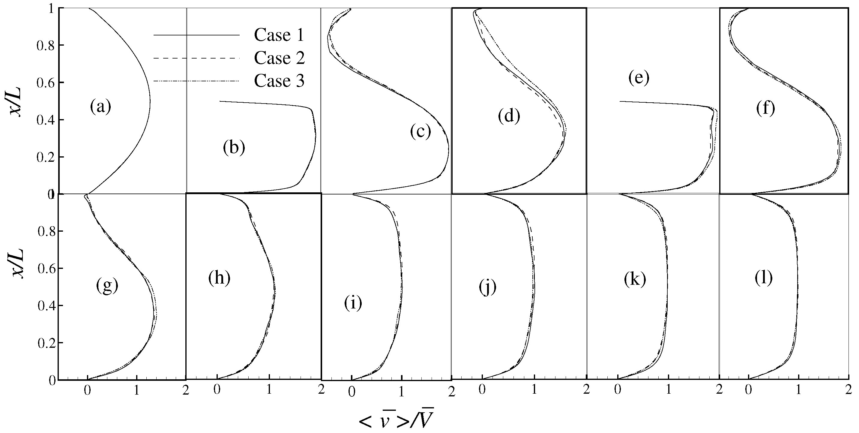
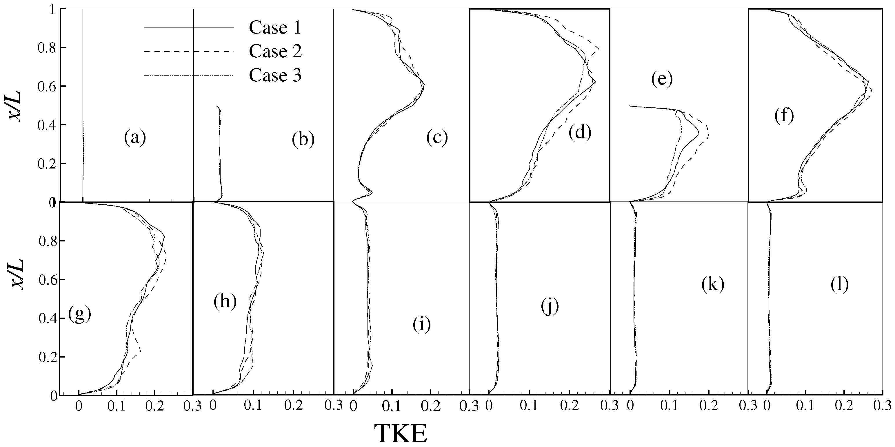
Figure 4 and Figure 5 show the grid independence test in terms of the mean streamwise velocity, v ¯ / V ¯ m a x , and the turbulent kinetic energy (TKE), 1 2 u j u j / V ¯ m a x 2 , at the different streamwise axial positions, while R e = 2000 . Three different grid arrangements used in the test are Case 1: 50 × 300 × 50 , Case 2: 50 × 350 × 50 and Case 3: 70 × 350 × 50 .
The mean streamwise velocity at the inlet of the channel (Figure 4a) where the flow is laminar and at the centre of the stenosis (Figure 4b) where the flow is going to be transitional is exactly the same for the different grid arrangements. However, the velocity slightly deviates at the position of the post lip of the first stenosis ((c) and (d)) where the permanent re-circulation region takes place. The velocity decreases slightly at y / L = 2.0 , but due to the presence of the second stenosis, it increases at the centre and post lip of the second stenosis. The negative velocity seen in (f) indicates the presence of another re-circulation region at the post lip of the second stenosis. After the second stenosis, the agreement of the velocity for the different grid arrangements is excellent. The maximum difference in the mean streamwise velocity is about 9% when changing the grid arrangement from Case 1 to 2 and from Case 1 to 3 is about 14% in the immediate post stenotic region at y / h = 2.0.
The turbulent kinetic energy in Figure 5 shows some variations after the stenoses, which are acceptable. Total grid independence of the computed turbulent random fluctuations is not expected in LES, and it is adequate to prove in LES that the primary flow features (mean velocities) do not vary significantly with the grid. Moreover, this dependence is apparent until the grid resolution becomes fine enough that the LES starts to qualify as DNS. Therefore, the grid arrangement of 50 × 300 × 50 seems fine to resolve the transient flow adequately in the double stenoses model. In (a) and (b), the turbulent kinetic energy (TKE) is almost zero as the flow is laminar upstream of the first stenosis. However, the effects of the second stenosis are clearly seen in frames (d) to (h). In the single-stenosis case, the maximum rise in TKE was observed in the post lip region, i.e., at y / L = 1.0 , which is shown in Molla et al. [23], but in the double stenoses case, it is seen that there is a sharp rise in TKE upstream and immediately downstream of the second stenosis. Finally, the TKE gradually decreases and approaches zero further downstream because of the re-laminarisation process, also seen for the single-stenosis model.
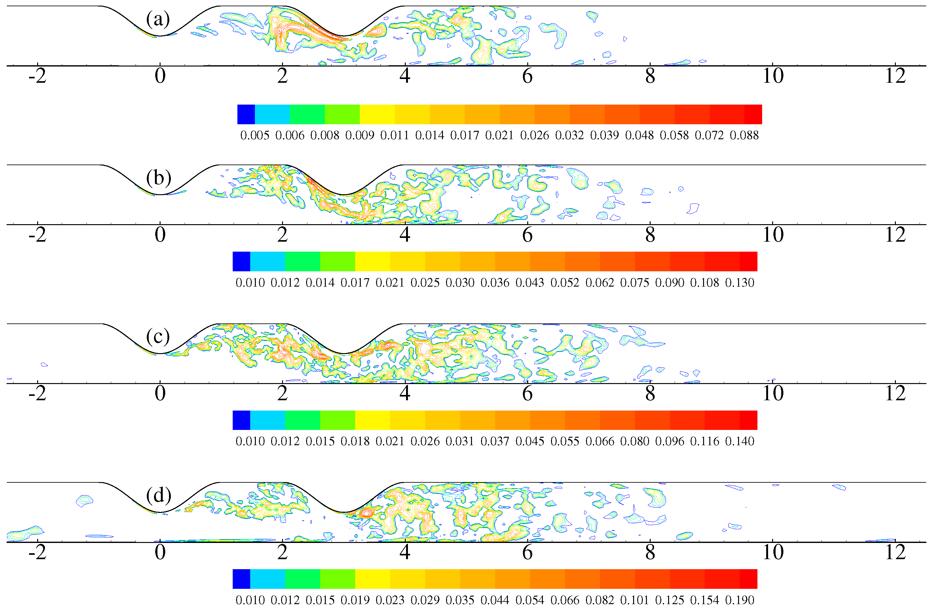
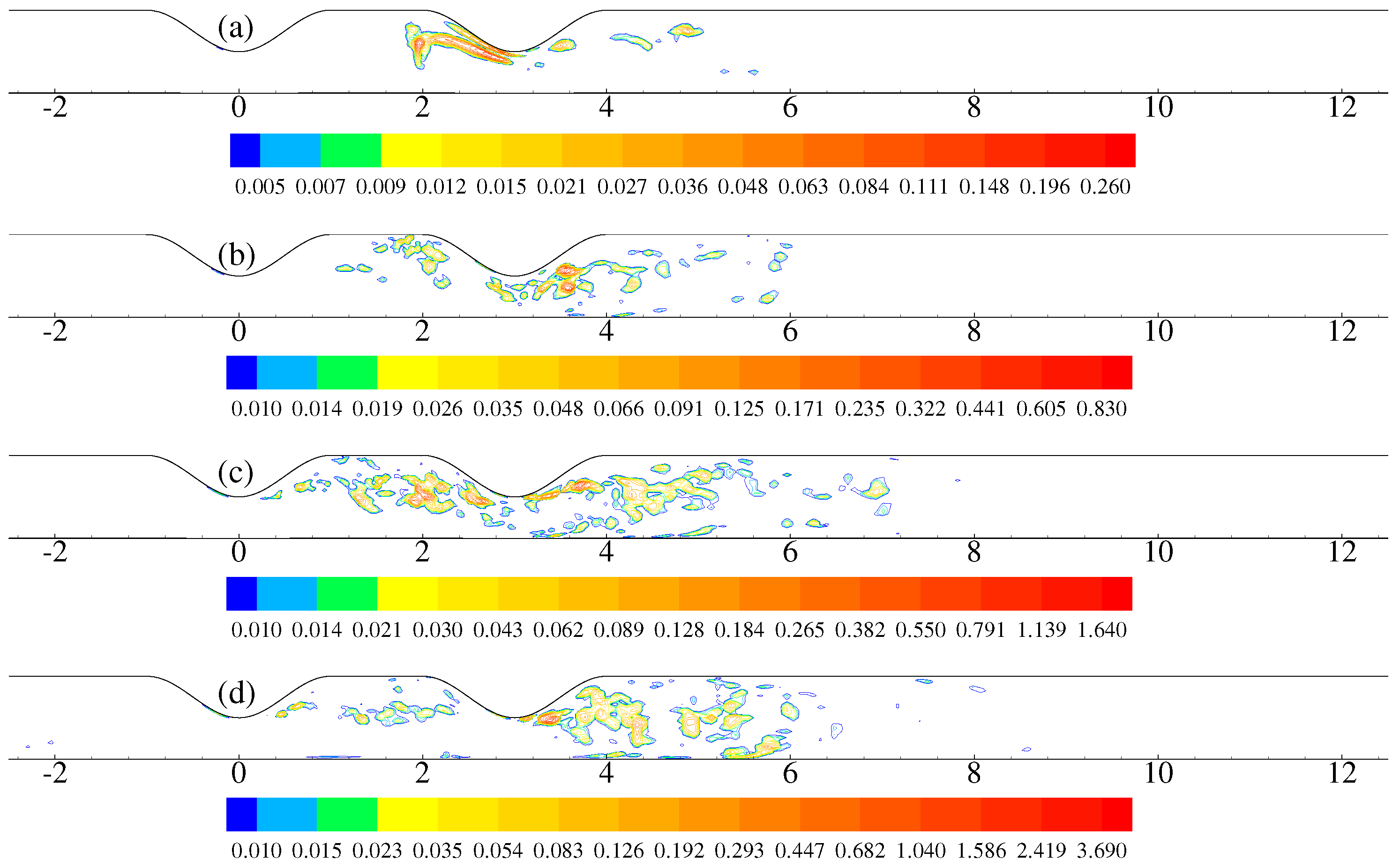
The dynamic values of the Smagorinsky constant C s are presented in Figure 6a–d for the different Reynolds numbers. The maximum values of C s , found near the throat and downstream of the second stenosis, are 0.088 , 0.13 , 0.14 and 0.19 , respectively, for R e = 1000 , 1400, 1700 and 2000. Due to the effects of the two stenoses, the values of the C s are almost doubled compared to those of the single stenosis in Molla et al. [23], while R e = 1700 and 2000, and the contribution from the SGS model, which is presented in Figure 7a,d in terms of the normalised SGS viscosity, increases in the second stenosis. Furthermore, the maximum SGS viscosity, μ s g s / μ , of 0.26 , 0.83 , 1.64 and 3.69 , obtained respectively for the Reynolds numbers above, corresponds to the large dissipation of the SGS model in the region of the second stenosis.
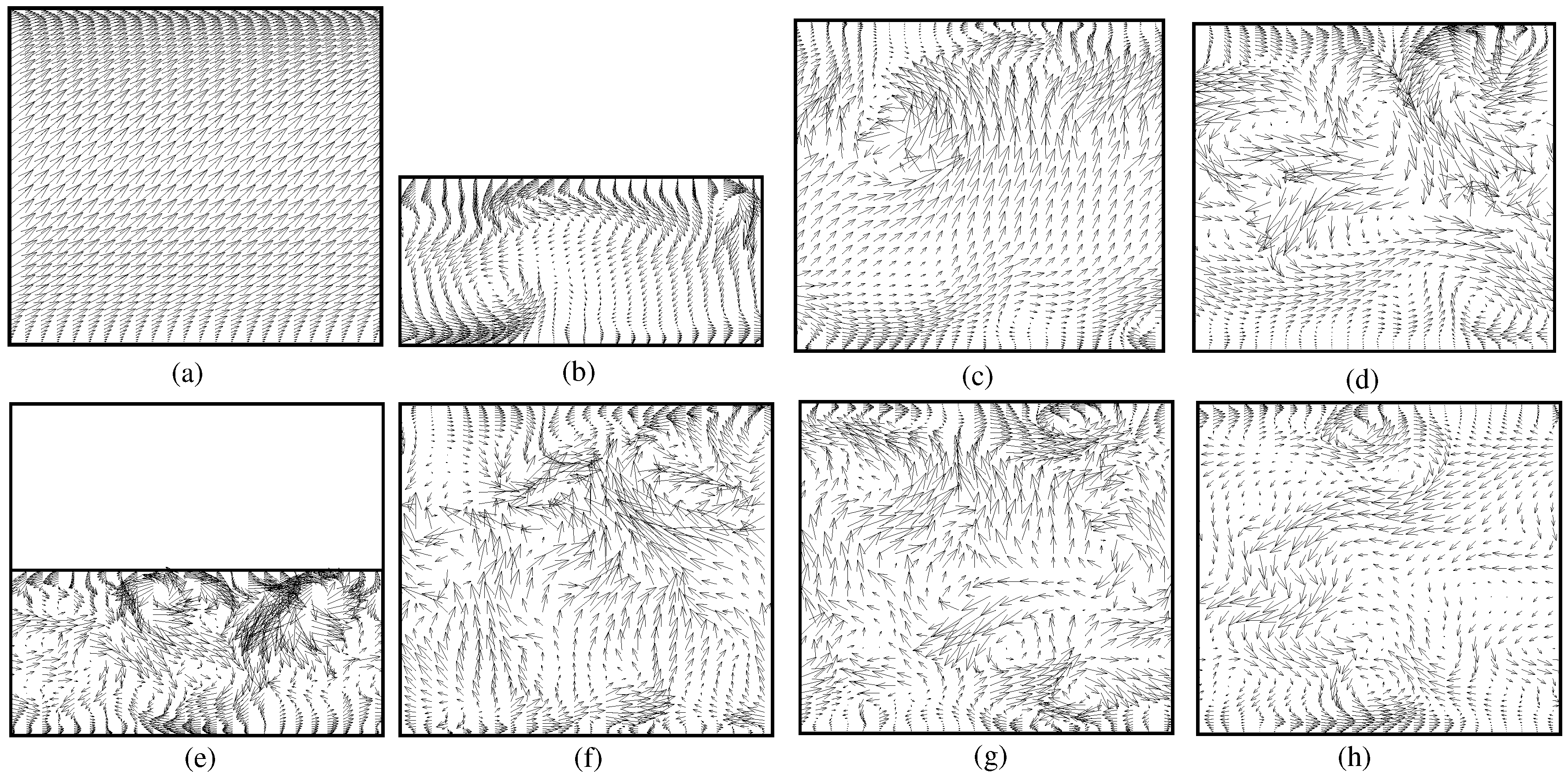
Figure 8a–h depict the instantaneous cross-stream velocity vectors at the different streamwise locations while R e = 2000 at t / T = 10.25 . At the inlet of the channel ( y / L = 5 ), the flow is laminar, while at the centre of the first stenosis ( y / L = 0 ), the flow is transitional to turbulent. At the post lip of the first stenosis ( y / L = 1 ), the recirculation is clearly visible near the upper wall where the turbulent intensity is higher than the lower wall. At y / L = 2 , the flow is fully turbulent, and the intensity of the turbulence increases at the centre of the second stenosis ( y / L = 3 ). After the second stenosis, the flow is too chaotic at ( y / L = 4 and 5) with a high intensity of turbulence. At the far downstream region, the intensity of the recirculation decreases gradually.
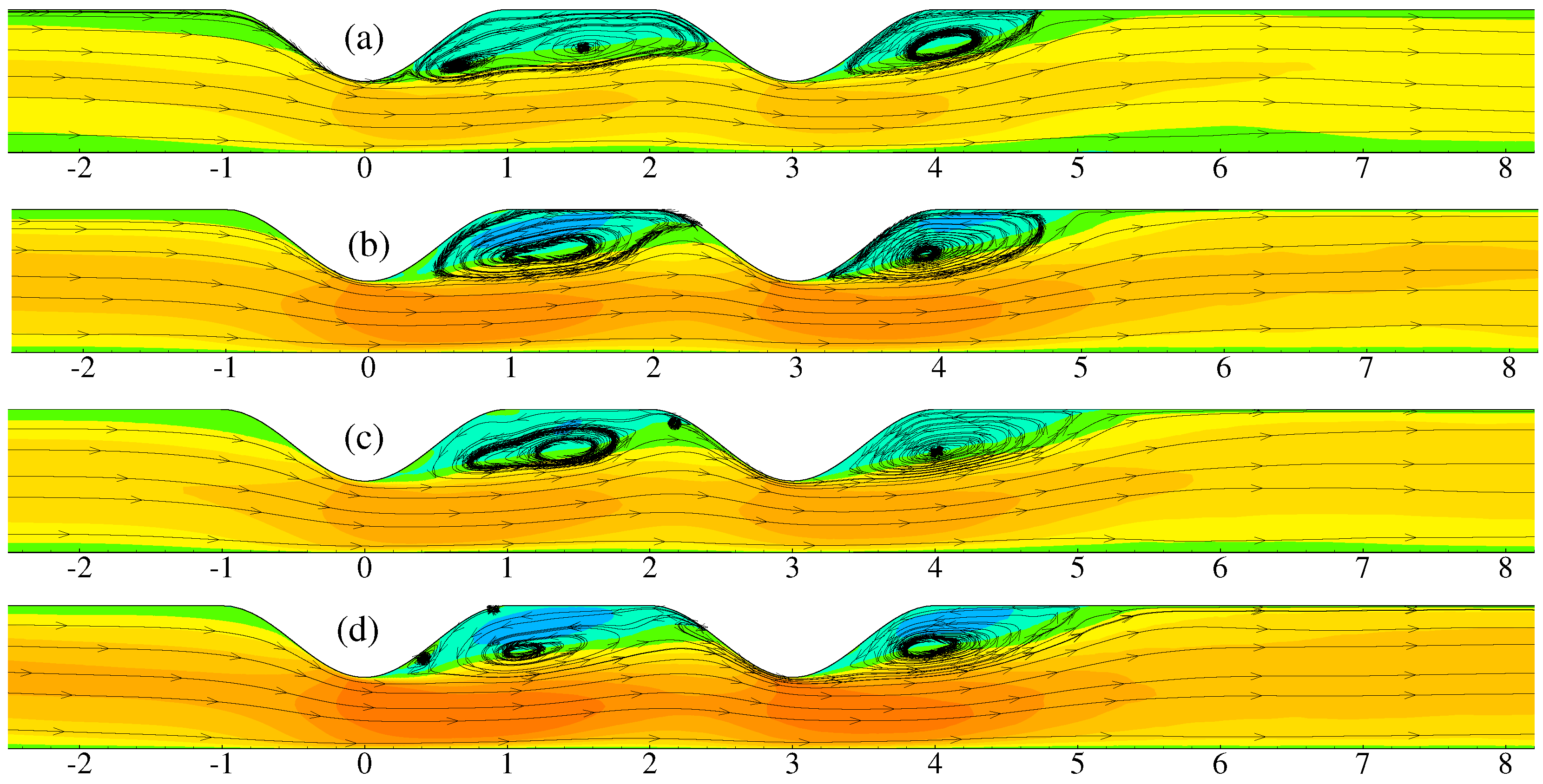
The mean streamlines appended on the mean streamwise velocity contours are presented in Figure 9a–d for the different Reynolds numbers. It is now clearly seen in this figure that there are two permanent re-circulation regions; the first one lies near the upper wall between the first and second stenoses, while the second re-circulation region lies at the post lip of the second stenosis. The length of these re-circulation regions also depends on the Reynolds number. For example, when R e = 1000 and 1400, the length of the first re-circulation region is larger than the second re-circulation region; whereas, the length of the second re-circulation region is larger than the first re-circulation region when R e = 1700 and 2000.
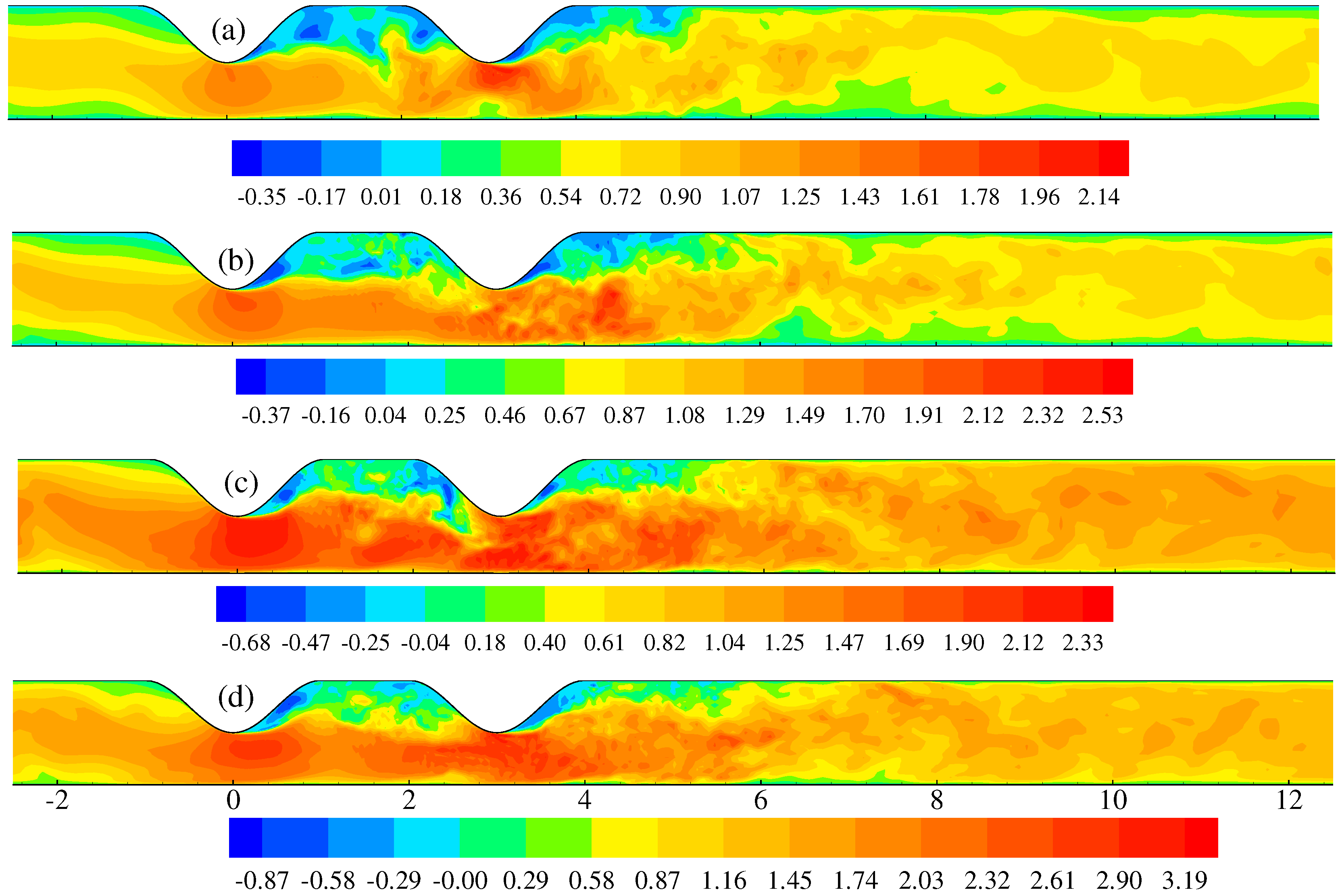
In order to understand more clearly the process of the flow separation from the nose of both stenoses and the region of the flow transition from laminar to turbulent, the instantaneous streamwise velocity v ¯ / V ¯ m a x is presented in Figure 10 for the different Reynolds numbers. Here, V ¯ m a x is the reference velocity calculated from R e = 2000 . The results show that the shear layer separated from the nose of the first stenosis is affected by the second stenosis and causes flow re-circulation near the upper wall between the two stenoses. The highly disturbed flow downstream of the second stenosis is caused by the separation of the shear layer from the second nose.
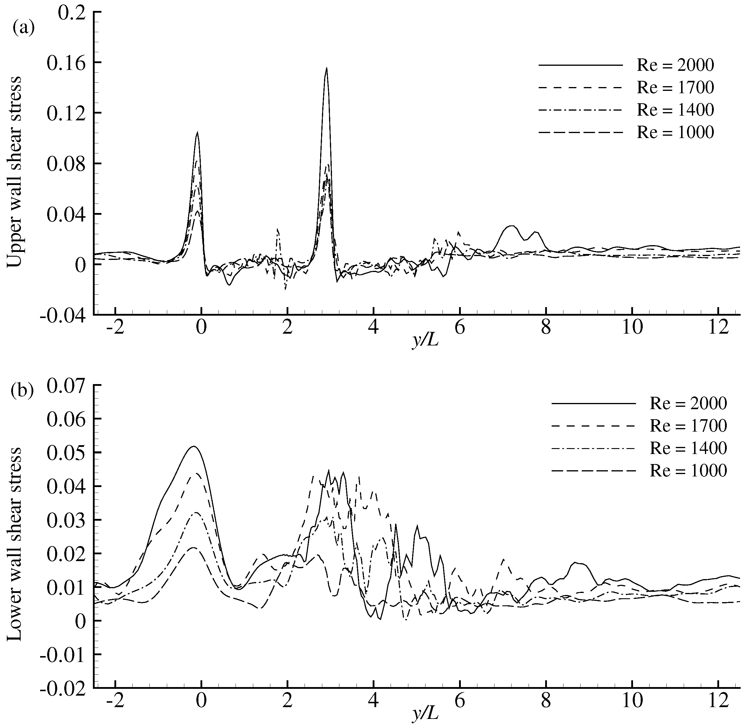
The instantaneous shear stress, τ w / ρ V ¯ m a x 2 , at the upper and lower walls is depicted in Figure 11a,b, respectively, for the different Reynolds numbers. At the upper wall, there are two levels of stress reduction; one takes place just prior to the centre of the first stenosis where flow is transitional, and the second one occurs just prior to the centre of the second stenosis where the flow is turbulent. The higher level of stress drop at the turbulent region can increase the tissue proliferation inside the arterial vessel and, consequently, increase the percentage of the stenosis. Therefore, the presence of multiple stenoses in an artery is more dangerous for a patient. In addition, the highly oscillating forms of the wall shear stress that occur at the second stenosis are more harmful to the blood cells (Sutera and Mehrjardi [38]) and blood vessels (Fry [39]).
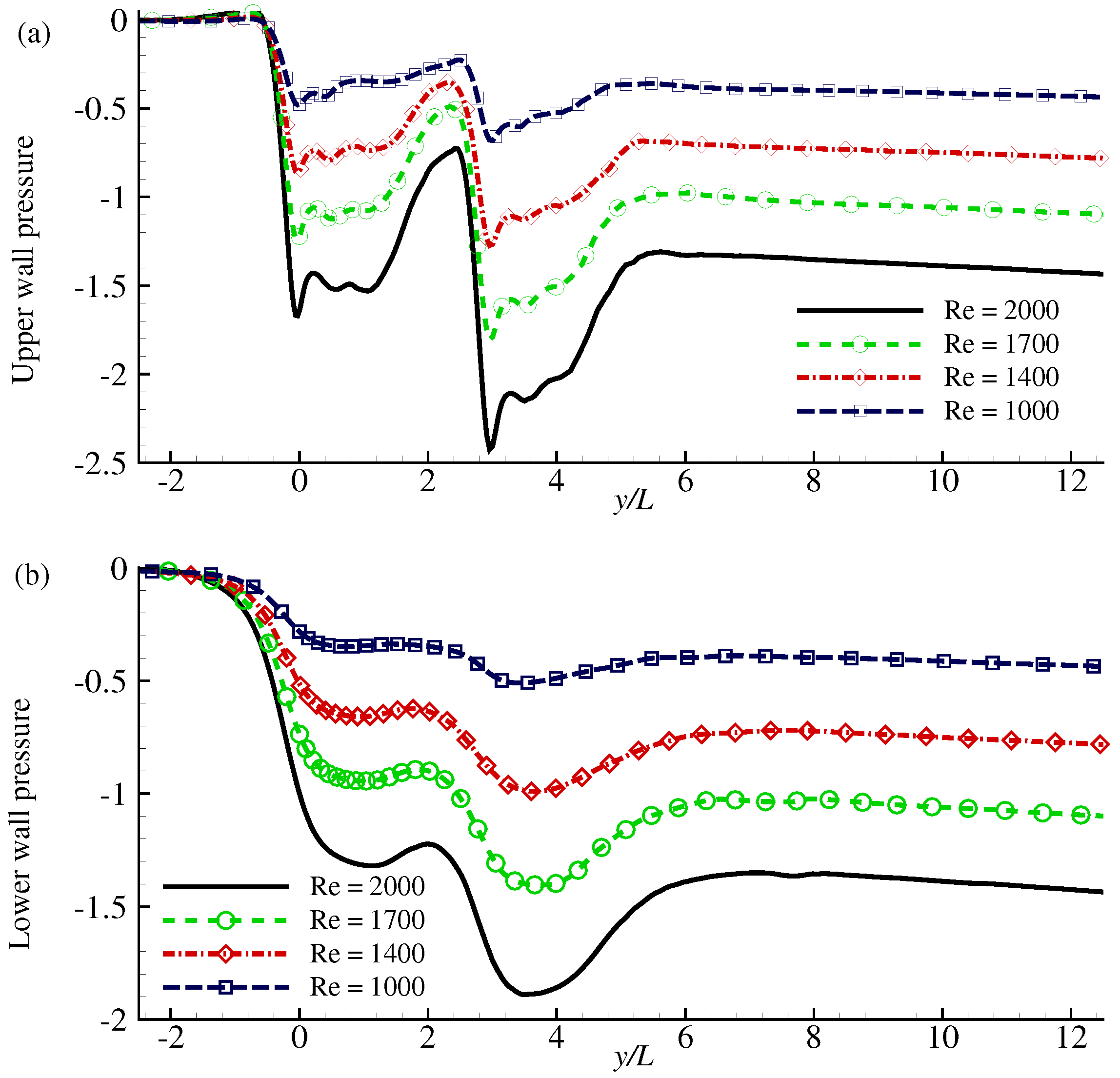
The effects of the multiple stenoses on the mean pressure, p ¯ / ρ V ¯ m a x 2 , at the upper and lower walls are illustrated respectively in Figure 12a,b. The effect of pressure drops at the centre of the stenoses is very acute near the upper wall due to the direct impact of the stenosis, while these are blunt in the case of the lower wall. Moreover, the effect is prominent in the second stenosis. The pressure drop in the second stenosis is larger than the first one, which again indicates the fact that the flow separated from the nose of the second stenosis re-circulates for a longer time than that of a single stenosis case. Consequently, the risk of thrombosis or stroke also increases.
The effects of the second stenosis on the turbulent flows are presented in this section in terms of the root mean square (rms) of the velocity and pressure fluctuations, as well as the energy spectra of the streamwise velocity fluctuations.
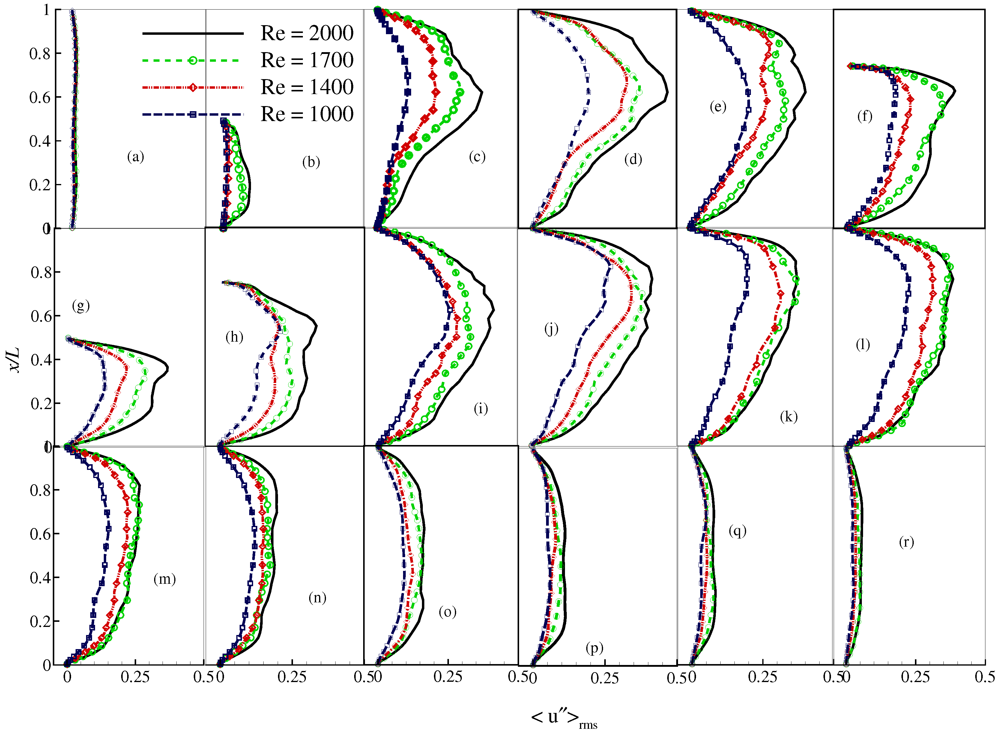
Figure 13 depicts the rms of the cross-stream velocity fluctuations, u r m s / V ¯ m a x , at the different axial locations for the different Reynolds numbers. The results show that at the centre of the first stenosis, y / L = 0.0 , the flow is transitional for R e = 1700 and 2000. The intensity of the cross-stream velocity fluctuations increases at the downstream of the first stenosis for all of the Reynolds numbers, and the maximum occurs at y / L = 1.5 . Although the intensity of the fluctuations reduces slightly at the pre lip of the second stenosis, y / L = 2.0 , due to the effects of the second stenosis, the fluctuations increase again in the downstream of the second stenosis near the upper wall. Further downstream, the turbulent fluctuations diminish in a similar manner as found in the single stenosis where the flow re-laminarises, which is also known as a recovery zone.
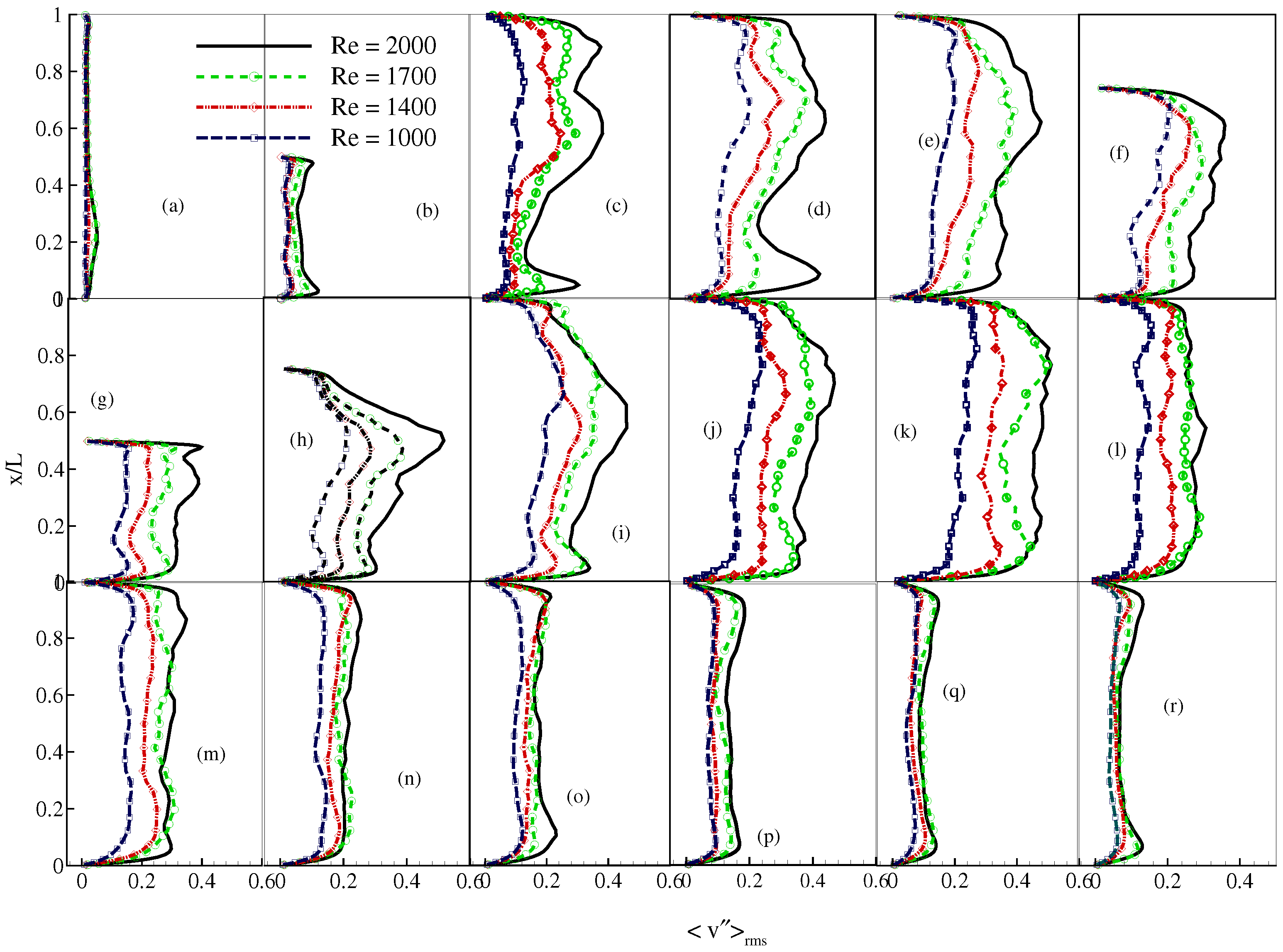
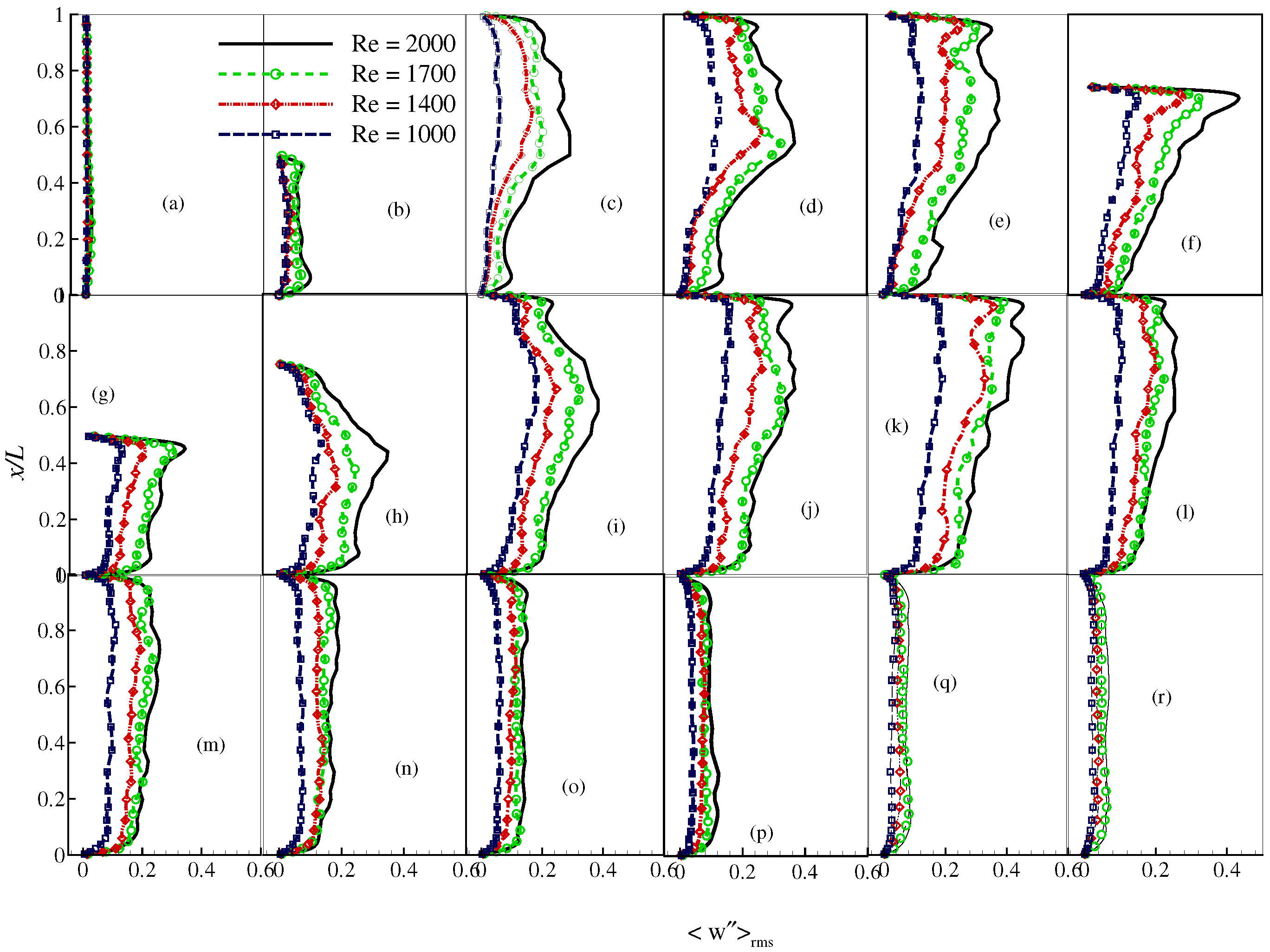
The rms values of the stream-wise and spanwise velocity turbulent fluctuations v r m s and w r m s at the different axial locations are plotted in Figure 14 and Figure 15, respectively. They are normalized by V ¯ m a x . The maximum value of v r m s is observed after the centre of the second stenosis at y / L = 3.5 , and the maximum value of w r m s / V ¯ m a x occurs before the centre of the second stenosis at y / L = 2.5 . Therefore, the presence of the second stenosis is pathologically important since it increases the turbulent intensity.
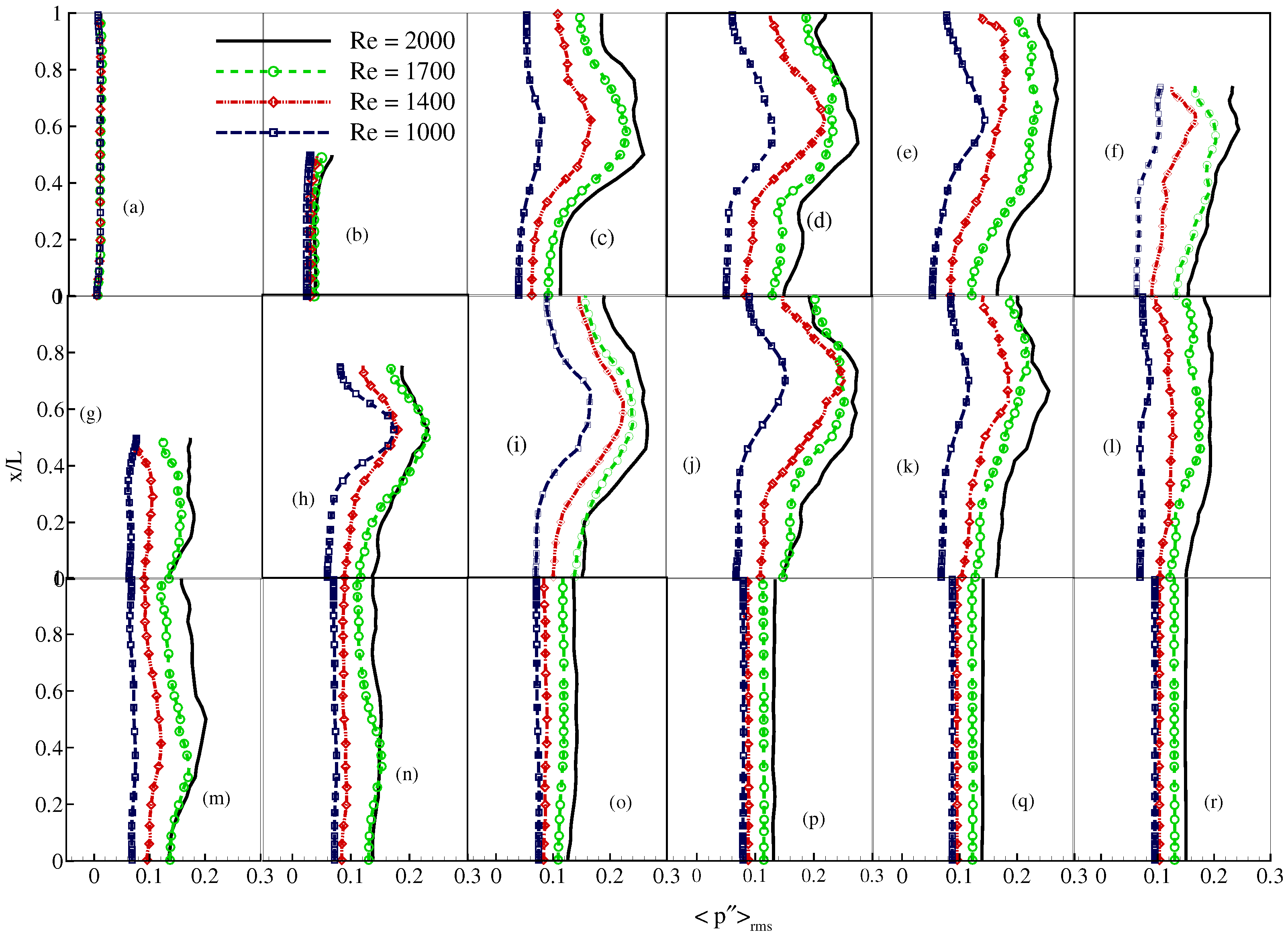
Another important turbulent quantity is the rms value of the pressure fluctuations presented in Figure 16. The pressure fluctuations after the immediate downstream region of the first stenosis are higher near the upper wall, but they mitigate slightly at the centre of the second stenosis. The magnitude of the fluctuations then increases rapidly up to the position of y / L = 4.5 , followed by a gradual decrease in the downstream. The high level of pressure fluctuations is responsible for the post stenotic dilatation due to the arterial damage, and these are also a potential source of arterial murmur, which is a key factor for identifying an arterial stenosis through acoustical techniques (Ask et al. [40]). The murmur due to the arterial stenosis is usually diagnosed by placing an external “transducer”, which transmits through the arterial wall. Since the presence of the double stenosis increases the magnitude of the pressure fluctuations, the intensity of the murmur sound from a double-stenosed artery would be higher than that of the single stenosis.
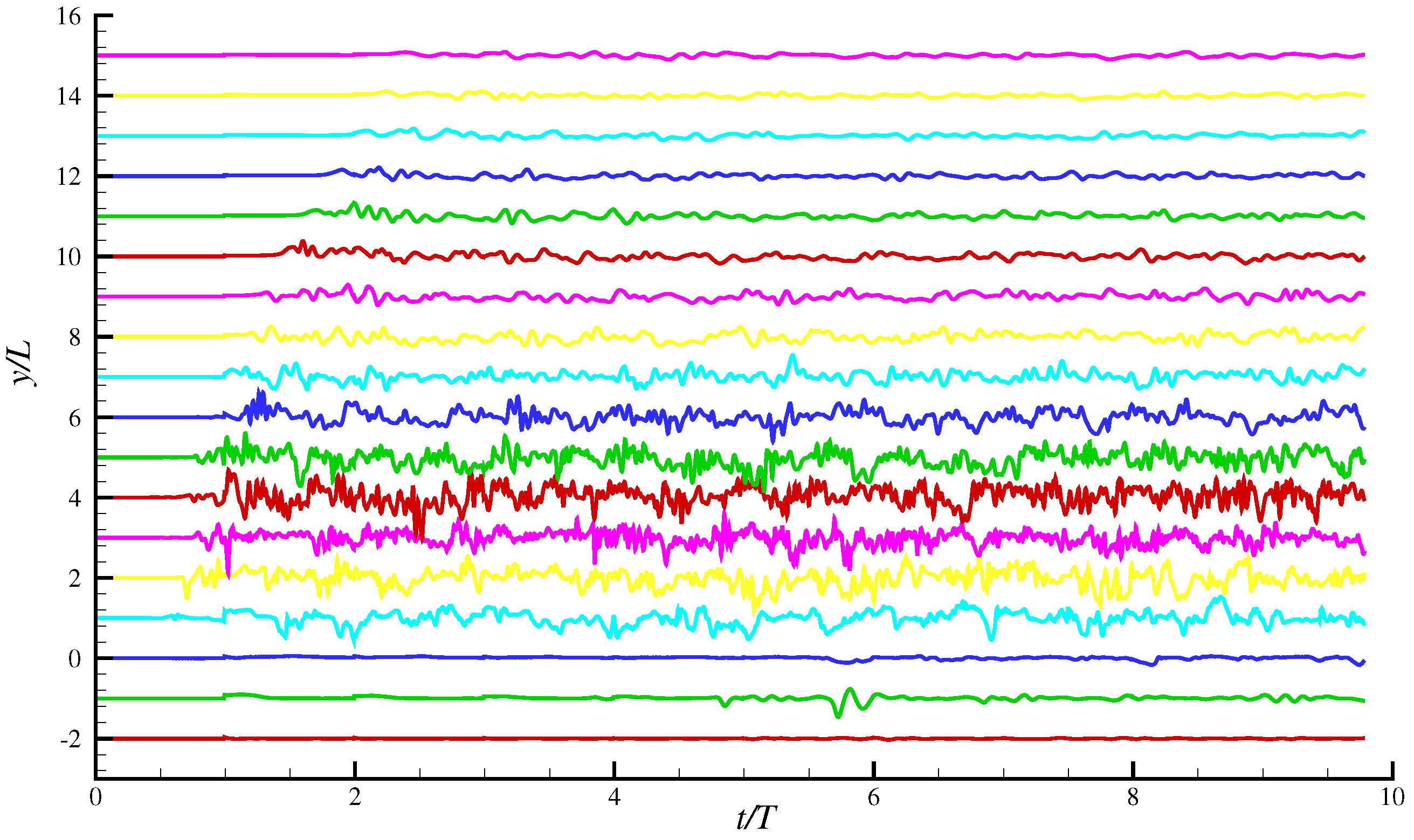
For understanding the laminar and turbulent flow region, the streamwise velocity fluctuations v / v m a x against the time period ( t / T , where T = 2 π ) at the different axial locations have been plotted in Figure 17. In Figure 17, y / L = 0 is the centre of the first stenosis, and y / L = 3 is the centre of the second stenosis. From this figure, it is clearly seen that the severe turbulence occurred after the second stenosis, and in the downstream region, the fluctuation is very low, which means the flow is going be re-laminarised.
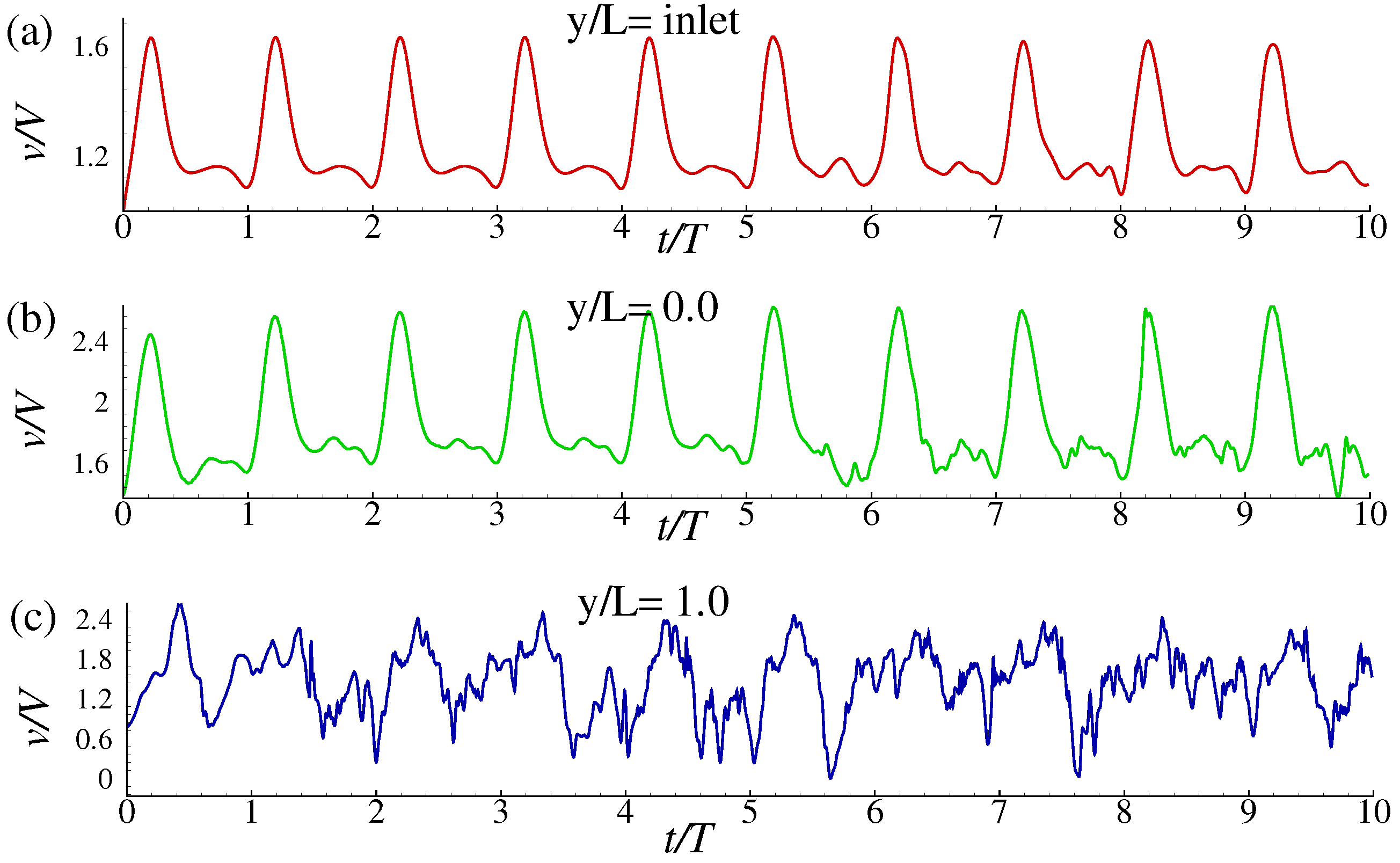
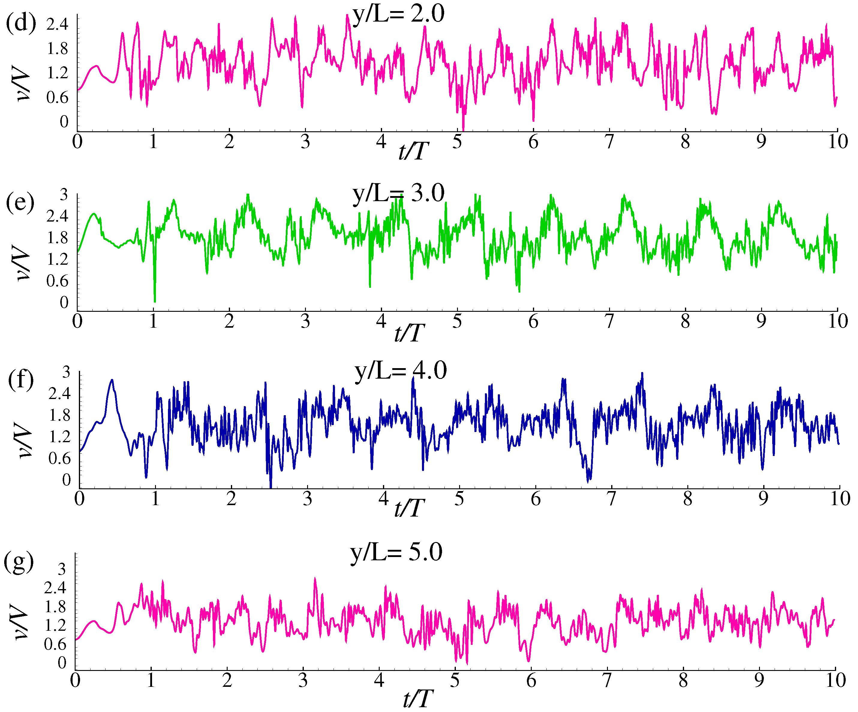
It has been tested that the mean and turbulent flow behaviour does not change over the pulse. However, the instantaneous flow changes over the pulse, and the maximum instantaneous wall shear stress occurs at the systolic phase at around t / T = 0.25 of the pulse. Mean and turbulent flow behaviour changes due to the presence of stenosis. Figure 18 shows the axial velocity behaviour over the pulse at the different axial locations. At the inlet, flow is laminar pulsatile, and at the centre of the first stenosis ( y / L = 0 ), the flow is not fully laminar, but may be transitional. At the first post stenotic region ( y / L = 1 and y / L = 2 ), it is not clearly distinguishable that turbulence peaks occur at the peak inlet flow or some other time instant. Similar turbulent flow patterns are visible at the centre of the second stenosis and the post stenotic region ( y / L = 3 , y / L = 4 , y / L = 5 , and so on).

5. Conclusions

In this paper, a large eddy simulation has been performed to investigate pulsatile flow through a square channel with two consecutive constrictions at the upper wall. In the previous studies for the single stenosis, it has been tested that the flow through the channel in the presence of stenosis is not fully turbulent. Before the stenosis, the flow is laminar, and at the throat of the stenosis, the flow might be transitional; as well as in the immediate post stenotic region, flow is turbulent. Therefore, it is not suitable to use a non-dynamic sub-grid scale (SGS) model for the laminar transition to turbulent flow, and consequently, the localized dynamic SGS model of Piomelli and Liu [29] has been used for the present simulations. From the results, it reveals that the effect of the SGS model before stenosis is almost zero at the laminar flow region.
The results presented in various forms show the effects of the presence of the second stenosis in an artery. For R e = 2000 , the maximum Smagorinsky constant obtained is C s 0.2 . The maximum contribution of the SGS model also increases at the region of the second stenosis. The upper wall pressure drops and wall shear stress increase rapidly in the region of stenoses for increasing the Reynolds numbers, which are consistent with the results of Talukder et al. [15] and Damodaran et al. [9]. It is clearly seen that the maximum pressure drops and wall shear stress occur due to the effects of the second stenosis.
Furthermore, due to the presence of the second stenosis, the turbulent intensity of the flow increases significantly. From the pathological point of view, the increment in the turbulent fluctuations is more dangerous, as they damage the material of blood cells and the inner surface of a blood vessel. The permanent re-circulation zone found in the downstream of the stenoses will also increase the risk of thrombosis or blood clotting and, consequently, increase the risk of heart attack or brain stroke.
For computational simplicity, a square channel with a rigid wall and with Newtonian blood flow is considered, which are the main limitations in this present research. We tried to give physical insight into the pulsatile blood flow in a model an artery with consecutive double stenoses. Even though the computational domain is a square channel, the results lead to the conclusion that the presence of multiple stenoses is harmful to patients.

Author Contributions

Md. Mamun Molla did the whole simulation and draft writing of this manuscript, and Manosh C. Paul supervised the entire research and edited the manuscript.

Conflicts of Interest

The authors declare no conflict of interest.

References

  1. Ku, D.N. Blood flows in arteries. Annu. Rev. Fluid Mech. 1997, 29, 399–434. [Google Scholar] [CrossRef]
  2. Khalifa, A.M.A.; Giddens, D.P. Analysis of disorder in pulsatile flows with application to poststenotic blood velocity measurement in dogs. J. Biomech. 1978, 11, 129–141. [Google Scholar] [CrossRef]
  3. Khalifa, A.M.A.; Giddens, D.P. Characterization and evolution of poststenotic flow disturbances. J. Biomech. 1981, 14, 279–296. [Google Scholar] [CrossRef]
  4. Clark, C. Turbulent velocity measurements in a model of aortic stenosis. J. Biomech. 1976, 9, 677–687. [Google Scholar] [CrossRef]
  5. O’Brien, V.; Ehrlich, L.W. Simple pulsatile flow in an artery with a constriction. J. Biomech. 1985, 18, 117–127. [Google Scholar] [CrossRef]
  6. Tutty, O.R. Pulsatile flow in a constricted channel. J. Biomech. Eng. 1992, 114, 50–54. [Google Scholar] [CrossRef] [PubMed]
  7. Tu, C.; Delville, M.; Dheur, L.; Vanderschure, L. Finite element simulation of pulsatile flow throgh arterial stenosis. J. Biomech. 1992, 25, 1141–1152. [Google Scholar] [CrossRef]
  8. Deplano, V.; Siouffi, M. Experimental and numerical study of pulsatile flows through stenosis: Wall shear stress analysis. J. Biomech. 1999, 32, 1081–1090. [Google Scholar] [CrossRef]
  9. Damodaran, V.; Rankin, G.W.; Zhang, C. Numerical study of steady laminar flow through tube with multiple constriction using curvilinear co-ordinates. Int. J. Numer. Meth. Fluids 1996, 23, 1021–1041. [Google Scholar] [CrossRef]
  10. Zendehbudi, G.R.; Moayeri, M.S. Comparison of physiogical and simple pulsatile flows through stenosed ateries. J. Biomech. 1999, 32, 959–965. [Google Scholar] [CrossRef]
  11. Dvinsky, A.S.; Ojha, M. Simulation of three-dimensional pulsatile flow through an asymmetric stenosis. Med. Biol. Eng. Comput. 1994, 32, 138–142. [Google Scholar] [CrossRef] [PubMed]
  12. Long, Q.; Xu, X.Y.; Ramnarine, K.V.; Hoskins, P. Numerical investigation of physiological realistic pulsatile flow through arterial stenosis. J. Biomech. 2001, 34, 1229–1242. [Google Scholar] [CrossRef]
  13. Mallinger, F.; Drikakis, D. Laminar-to-turbulent transition in pulsatile flow through a stenosis. Biorheology 2002, 39, 437–441. [Google Scholar] [PubMed]
  14. Mallinger, F.; Drikakis, D. Instability in three-dimensional, unsteady, stenotic flows. Int. J. Heat Fluid Flow 2002, 23, 657–663. [Google Scholar] [CrossRef]
  15. Talukder, N.; Karayannacos, P.E.; Nerem, R.M.; Vasco, J.S. An experimental study of fluid mechanics of arterial stenosis. J. Biomech. Eng. 1977, 99, 74–82. [Google Scholar] [CrossRef]
  16. Lee, T.S.; Liao, W.; Low, H.T. Numerical simulation of turbulent flow through series stenoses. Int. J. Numer. Meth. Fluids 2003, 42, 717–740. [Google Scholar] [CrossRef]
  17. Lee, T.S.; Liao, W.; Low, H.T. Numerical study of physiological turbulent flows through series arterial stenoses. Int. J. Numer. Meth. Fluids 2004, 46, 315–344. [Google Scholar] [CrossRef]
  18. Varghese, S.S.; Frankel, S.H. Numerical Modeling of Pulsatile Turbulent Flow in Stenotic Vessels. J. Biomch. Eng. 2003, 125, 445–460. [Google Scholar] [CrossRef]
  19. Varghese, S.S.; Frankel, S.H.; Fischer, P.F. Direct numerical simulation of stenotic flows. Part 2. Pulsatile flow. J. Fluid Mech. 2007, 582, 281–318. [Google Scholar] [CrossRef]
  20. Scotti, A.; Piomelli, U. Turbulence models in pulsatile flow. AIAA J. 2002, 40, 537–544. [Google Scholar] [CrossRef]
  21. Paul, M.C.; Molla, M.M.; Roditi, G. Large-eddy simulation of pulsatile blood flow. Med. Eng. Phys. 2009, 31, 153–159. [Google Scholar] [CrossRef] [PubMed]
  22. Paul, M.C.; Molla, M.M. Investigation of physiological pulsatile flow in a model arterial stenosis using large-eddy and direct numerical simulations. Appl. Math. Model. 2012, 36, 4393–4413. [Google Scholar] [CrossRef]
  23. Molla, M.M.; Paul, M.C.; Roditi, G. LES of additive and non-additive pulsatile flows in a model arterial stenosis. Comput. Methods Biomech. Biomed. Eng. 2010, 13, 105–120. [Google Scholar] [CrossRef]
  24. Molla, M.M.; Wang, B.C.; Kuhn, D.C.S. Numerical study of pulsatile channel flows undergoing transition triggered by a modelled stenosis. Phys. Fluid 2012, 24, 121901. [Google Scholar] [CrossRef]
  25. Molla, M.M.; Hossain, A.; Wang, B.C.; Kuhn, D.C.S. Large-eddy simulation of pulsatile non-Newtonian flow in a constricted channel. Prog. Comput. Fluid Dyn. 2012, 12, 231–241. [Google Scholar] [CrossRef]
  26. Molla, M.M.; Paul, M.C. LES of non-Newtonian physiological blood flow in a model of arterial stenosis. Med. Eng. Phys. 2012, 34, 1079–1087. [Google Scholar] [CrossRef] [PubMed]
  27. Piomelli, U.; Liu, J. Large-eddy simulation of rotating channel flows using a localized dynamic model. Phys. Fluids 1995, 7, 839–848. [Google Scholar] [CrossRef]
  28. Smagorinsky, J. General circulation experiment with the primitive equations. I. The basic experiment. Mon. Weather Rev. 1963, 91, 99–164. [Google Scholar] [CrossRef]
  29. Piomelli, U.; Liu, J. Large-eddy simulation of rotating channels flows using a localized dynamic model. Phys. Fluids 1994, 7, 839–847. [Google Scholar] [CrossRef]
  30. Womersley, J.R. Method for the calculation of velocity, rate of flow and viscous drag in arteris when the pressure gradient is known. J. Physiol. 1955, 155, 553–563. [Google Scholar] [CrossRef]
  31. Thomson, J.F.; Thames, F.; Mastin, C. Automatic numerical generation of body-fitted curvilinear coordinates system for field containing any number of arbitrary two dimensional bodies. J. Comput. Phys. 1974, 15, 299–319. [Google Scholar] [CrossRef]
  32. Morinishi, Y. Conservation Prperties of Finite Difference Schemes For Incompressible Flow; Center for Turbulence Research: Stanford, CA, USA, 1995; pp. 121–132. [Google Scholar]
  33. Patankar, S.V. Numerical Heat Transfer and Fluid Fow; Hemisphere Publishing Corporation: New York, NY, USA, 1980. [Google Scholar]
  34. Rhie, C.M.; Chow, W.L. Numerical study of the turbulent flow past an airfoil with trailing edge separation. AIAA J. 1983, 21, 1525–1532. [Google Scholar] [CrossRef]
  35. Vorst, H.A.D. BI-CGSTAB: A first and smoothly converging variant of BI-CG for the solution of the non-symmetric linear systems. SIAM J. Sci. Stat. Comput. 1992, 13, 631–644. [Google Scholar] [CrossRef]
  36. Kershaw, D.S. The Incomplete Cholesky-Cojugate Gradient method for the iterative solution of systems. J. Comput. Phys. 1978, 26, 43–65. [Google Scholar] [CrossRef]
  37. Jones, W.P.; di Mare, F.; Marquis, A.J. LES-BOFFIN: User’s Guide; Imperial College: London, UK, 2002. [Google Scholar]
  38. Sutera, S.P.; Mehrjardi, M.H. Deformation and fragmentation of human red blood cells in turbulent flow. Biophys. J. 1975, 15, 1–10. [Google Scholar] [CrossRef]
  39. Fry, D.L. Acute vascular endothelial changes associated with increases blood velocity gradients. Circ. Res. 1968, 22, 165–197. [Google Scholar] [CrossRef] [PubMed]
  40. Ask, P.; Hok, B.; Loyd, D.; Terio, H. Bio-acoustic signals from stenotic tube flow: State of the art and perspectives for future methodological development. Med. Biol. Eng. Comput. 1995, 33, 669–675. [Google Scholar] [CrossRef] [PubMed]
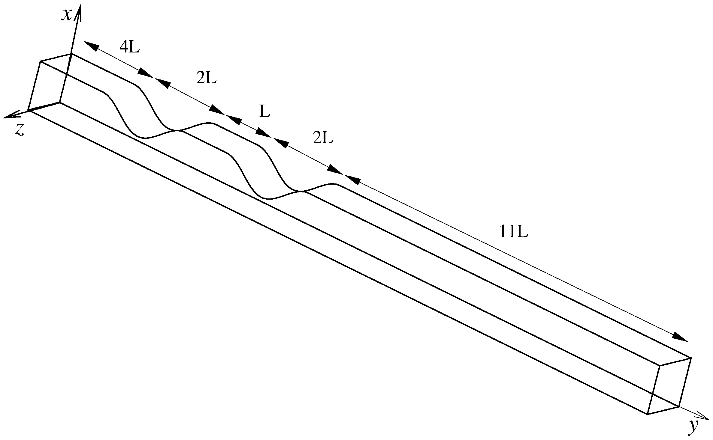
Figure 1. A schematic of the model with the coordinate system.
Fluids 02 00001 g001
Figure 2. A crude mesh distribution in the x y plane.
Fluids 02 00001 g002
Figure 3. Streamwise inlet velocity v ¯ / V ¯ m a x (a) near the wall x / L = 0.0057 , (b) at the centre of the channel x / L = 0.5 and (c) at the different phases of the pulse while R e = 2000 .
Fluids 02 00001 g003
Figure 4. Grid independence test for the mean streamwise velocity, v ¯ / V ¯ m a x , at (a) y / L = inlet, (b) y / L = 0.0 , (c) y / L = 1.0 , (d) y / L = 2.0 , (e) y / L = 3.0 , (f) y / L = 4.0 , (g) y / L = 5.0 , (h) y / L = 6.0 , (i) y / L = 8.0 , (j) y / L = 10.0 , (k) y / L = 12.0 and (l) y / L = outlet, while R e = 2000 , Case 1: 50 × 300 × 50 , Case 2: 50 × 350 × 50 and Case 3: 70 × 350 × 50 control volumes.
Fluids 02 00001 g004
Figure 5. Grid independence test for the turbulent kinetic energy (TKE), 1 2 u j u j / V ¯ m a x 2 , (a) y / L = inlet, (b) y / L = 0.0 , (c) y / L = 1.0 , (d) y / L = 2.0 , (e) y / L = 3.0 , (f) y / L = 4.0 , (g) y / L = 5.0 , (h) y / L = 6.0 , (i) y / L = 8.0 , (j) y / L = 10.0 , (k) y / L = 12.0 and (l) y / L = outlet, while R e = 2000 ; Case 1: 50 × 300 × 50 , Case 2: 50 × 350 × 50 and Case 3: 70 × 350 × 50 control volumes.
Fluids 02 00001 g005
Figure 6. Dynamic Smagorinsky constant, C s , for (a) R e = 1000 , (b) R e = 1400 , (c) R e = 1700 and (d) R e = 2000 at t / T = 10.25 .
Fluids 02 00001 g006
Figure 7. Normalised sub-grid scale (SGS) eddy viscosity, μ s g s / μ , for (a) R e = 1000 , (b) R e = 1400 , (c) R e = 1700 and (d) R e = 2000 at t / T = 10.25 .
Fluids 02 00001 g007
Figure 8. Instantaneous cross-stream velocity vectors based on the velocity components u ¯ v ¯ , (a) y / L = inlet, (b) y / L = 0.0 , (c) y / L = 1.0 , (d) y / L = 2.0 , (e) y / L = 3.0 , (f) y / L = 4.0 , (g) y / L = 6.0 and (h) y / L = 8.0 while R e = 2000 .
Fluids 02 00001 g008
Figure 9. Mean streamwise streamlines appended on the mean streamwise velocity, < v ¯ > / V ¯ m a x , for (a) R e = 1000 , (b) R e = 1400 , (c) R e = 1700 and (d) R e = 2000 .
Fluids 02 00001 g009
Figure 10. Contour plot of the instantaneous streamwise velocity, v ¯ / V ¯ m a x , for (a) R e = 1000 , (b) R e = 1400 , (c) R e = 1700 and (d) R e = 2000 at t / T = 10.25 .
Fluids 02 00001 g010
Figure 11. Instantaneous wall shear stress, τ w / ρ V ¯ m a x 2 , at the (a) upper wall and (b) lower wall for the different Reynolds numbers at t / T = 10.25 .
Fluids 02 00001 g011
Figure 12. Time-mean pressure, p ¯ / ρ V ¯ m a x 2 , at the (a) upper wall and (b) lower wall for the different Reynolds numbers.
Fluids 02 00001 g012
Figure 13. rms of the cross-stream velocity fluctuations, u r m s / V ¯ m a x , at the different axial locations: (a) y / L = inlet, (b) y / L = 0.0 , (c) y / L = 1.0 , (d) y / L = 1.5 , (e) y / L = 2.0 , (f) y / L = 2.5 , (g) y / L = 3.0 , (h) y / L = 3.5 , (i) y / L = 4.0 , (j) y / L = 4.5 , (k) y / L = 5.0 , (l) y / L = 5.5 , (m) y / L = 6.0 , (n) y / L = 7.0 , (o) y / L = 8.0 , (p) y / L = 10.0 , (q) y / L = 12.0 and (r) y / L = outlet, for the different Reynolds numbers.
Fluids 02 00001 g013
Figure 14. rms of the streamwise velocity fluctuations, v r m s / V ¯ m a x , at the different axial locations: (a) y / L = inlet, (b) y / L = 0.0 , (c) y / L = 1.0 , (d) y / L = 1.5 , (e) y / L = 2.0 , (f) y / L = 2.5 , (g) y / L = 3.0 , (h) y / L = 3.5 , (i) y / L = 4.0 , (j) y / L = 4.5 , (k) y / L = 5.0 , (l) y / L = 5.5 , (m) y / L = 6.0 , (n) y / L = 7.0 , (o) y / L = 8.0 , (p) y / L = 10.0 , (q) y / L = 12.0 and (r) y / L = outlet, for the different Reynolds numbers.
Fluids 02 00001 g014
Figure 15. rms of the spanwise velocity fluctuations, w r m s / V ¯ m a x , at the different axial locations: (a) y / L = inlet, (b) y / L = 0.0 , (c) y / L = 1.0 , (d) y / L = 1.5 , (e) y / L = 2.0 , (f) y / L = 2.5 , (g) y / L = 3.0 , (h) y / L = 3.5 , (i) y / L = 4.0 , (j) y / L = 4.5 , (k) y / L = 5.0 , (l) y / L = 5.5 , (m) y / L = 6.0 , (n) y / L = 7.0 , (o) y / L = 8.0 , (p) y / L = 10.0 , (q) y / L = 12.0 and (r) y / L = outlet, for the different Reynolds numbers.
Fluids 02 00001 g015
Figure 16. rms of the pressure fluctuations, p r m s / ρ V ¯ m a x 2 , at the different axial locations: (a) y / L = inlet, (b) y / L = 0.0 , (c) y / L = 1.0 , (d) y / L = 1.5 , (e) y / L = 2.0 , (f) y / L = 2.5 , (g) y / L = 3.0 , (h) y / L = 3.5 , (i) y / L = 4.0 , (j) y / L = 4.5 , (k) y / L = 5.0 , (l) y / L = 5.5 , (m) y / L = 6.0 , (n) y / L = 7.0 , (o) y / L = 8.0 , (p) y / L = 10.0 , (q) y / L = 12.0 and (r) y / L = outlet, for the different Reynolds numbers.
Fluids 02 00001 g016
Figure 17. Streamwise velocity fluctuations v / v m a x against the time cycle t / T of pulsation at the different axial locations while R e = 2000 and x / L = z / L = 0.5 .
Fluids 02 00001 g017
Figure 18. Streamwise velocity v / V ¯ m a x against the time cycle t / T of pulsation at (a) y / L = inlet, (b) y / L = 0 (centre of the first stenosis), (c) y / L = 1.0, (d) y / L = 2.0, (e) y / L = 3.0 (centre of the second stenosis), (f) y / L = 4.0 and (g) y / L = 5.0, while R e = 2000 and x / L = z / L = 0.5 .
Fluids 02 00001 g018aFluids 02 00001 g018b
Table 1. Values of M n and ϕ n for different harmonics according to Womersley [30].
N h M n ϕ n
1 0.78 0.0113446
2 1.32 1.4442599
3 0.74 0.4625122
4 0.41 0.2879793
Table 2. Mesh details used in the computations.
Case Re N x N y N z Δ t
0<20005030050 10 3
120005030050 10 3
220005035050 10 3
320007035050 10 3