Hexagonal Cell Formation in Darcy–Bénard Convection with Viscous Dissipation and Form Drag

Abstract

Recent interest in the effects of viscous dissipation on convective flows in porous media has centred almost exclusively on forced convection flows. In this paper, we investigate the manner in which it affects the onset and early stages of convection in Darcy–Bénard convection. A weakly nonlinear theory is described briefly, and it is shown that hexagonal cells are preferred over rolls when the Rayleigh number is sufficiently close to 4${\pi }^2$. At higher Rayleigh numbers, two-dimensional rolls are preferred. When weak form drag is included, then subcritical convection eventually disappears as the Forchheimer parameter increases, yielding a highly novel situation wherein hexagonal convection arises supercritically. The range of stability of hexagons is found to increase.

1. Introduction

The problem of the onset and development of convection in a uniform horizontal layer heated from below is known as the Darcy–Bénard problem or the Horton–Rogers–Lapwood problem, and it has been studied widely since the pioneering works of Horton and Rogers [1] and Lapwood [2]. Detailed accounts of the development of the subject may be found in the reviews by Nield and Bejan [3], Rees [4], Tyvand [5] and Barletta [6].

In its classical form Darcy’s law applies, which means that there are no extensions such as those represented by the boundary and form-drag terms, an anisotropy permeability or temperature-dependent properties. Likewise, the heat transport equation does not include thermal dispersion terms, an anisotropic diffusivity, a temperature-dependent viscosity or local thermal nonequilibrium effects. In this original form, and in an unbounded layer, the critical Rayleigh number is very well-known to be $4{\pi }^2$ and the associated wavenumber is $\pi$ [1,2]. Weakly nonlinear theory then shows that two-dimensional rolls are favoured; three-dimensional planforms such as rectangular or hexagonal cells are unstable and therefore unachievable in practice. There are contexts when this straightforward scenario is altered—these include layers with discrete sublayers (square cells; see Rees and Riley [7]), layers with imperfectly conducting boundaries (also square cells; Riahi [8] and Rees and Mojtabi [9]), layers with spatially varying boundary temperatures (rectangles, wavy rolls; see Rees and Riley [10,11]), and layers with internal heating (hexagonal cells; see Tveitereid [12]).

In this paper, we consider the combined effects of viscous dissipation and form-drag (also called the Forchheimer effect) on weakly nonlinear convection in an otherwise classical Darcy–Bénard layer. While one could have chosen a different pair of “effects”, these two are found to interact in a somewhat unusual manner, and therefore it is these which will be considered. At present, there is only one paper to our knowledge that considers the effect of viscous dissipation in the nonlinear regime in the context of thermoconvective instability, and that is the analysis by Celli et al. [13] who consider mixed convection in a Darcy–Bénard layer. Their externally-induced and uniform horizontal flow is parallel to the axes of the convecting cells. One further paper which is of some interest in the present context is that of Rees [14], which considers the presence of viscous dissipation in a sidewall-heated square cavity. In that work, the author showed that the “velocity-squared” model for viscous dissipation in a porous medium, the form which is generally used and which was derived by Breugem and Ree [15] using a Representative Elementary Volume analysis, cannot be sustained by having values for the Gebhart number that are too large. In [14], it was found that, when Gebhart number increases beyond a critical value (which depends on the Rayleigh number but which is above unity), then there exists a region within the interior of the cavity that has temperatures that are larger than what is imposed on the boundary, a situation which is unphysical. Thus, large Gebhart numbers induce a physical situation that cannot occur in reality, and this concurs with the following statement by Celli et al. [12], namely, that: the condition Ge=1 is far beyond any conceivable application, except for some geophysical cases. In the present paper, the Gebhart number is assumed to be asymptotically small, and its magnitude is used as the expansion parameter for the weakly nonlinear analysis.

It is shown that a hexagonal pattern of convection is preferred when convection first appears, and that this is due to the presence of viscous dissipation which introduces extra forcing terms at third order in the weakly nonlinear theory. At higher Rayleigh numbers within the weakly nonlinear regime, rolls are re-established as the favoured pattern, although there is an intermediate regime where both patterns are stable to small disturbances. It is found that, as the Forchheimer parameter increases from zero, hexagonal cells lose their characteristic subcriticality, but they increase their range of stability to small disturbances.

The analysis which is followed here is based heavily on the general framework for the weakly nonlinear theory of Darcy–Bénard convection, which is outlined in Rees [16], and the reader is referred to those lecture notes for further details.

2. Governing Equations

The equations governing Boussinesq convection in a porous medium subject to Darcy’s law are given by

$${\displaystyle \frac{\partial \overline{u}}{\partial \overline{x}}}+{\displaystyle \frac{\partial \overline{v}}{\partial \overline{y}}}+{\displaystyle \frac{\partial \overline{w}}{\partial \overline{z}}}=0,$$

(1)

$$\overline{u}=-\frac{K}{\mu }{\displaystyle \frac{\partial \overline{p}}{\partial \overline{x}}},\overline{v}=-\frac{K}{\mu }{\displaystyle \frac{\partial \overline{p}}{\partial \overline{y}}},\overline{w}=-\frac{K}{\mu }{\displaystyle \frac{\partial \overline{p}}{\partial \overline{z}}}+\frac{{\rho }_{f}g\beta K}{\mu }\left(T-T_{\min }\right),$$

(2)

$${\left(\rho C_p\right)}_m{\displaystyle \frac{\partial T}{\partial \overline{t}}}+{\left(\rho C_p\right)}_f\left[\overline{u}{\displaystyle \frac{\partial T}{\partial \overline{x}}}+\overline{v}{\displaystyle \frac{\partial T}{\partial \overline{y}}}+\overline{w}{\displaystyle \frac{\partial T}{\partial \overline{z}}}\right]=k\left[{\displaystyle \frac{{\partial }^{2}T}{\partial {\overline{x}}^2}}+{\displaystyle \frac{{\partial }^{2}T}{\partial {\overline{y}}^2}}+{\displaystyle \frac{{\partial }^{2}T}{\partial {\overline{z}}^2}}\right]+\frac{\mu }{K}[{\overline{u}}^2+{\overline{v}}^2+{\overline{w}}^2],$$

(3)

where K is the permeability, g gravity, $\mu$ the fluid viscosity, k the thermal conductivity of the saturated medium and $\beta$ the coefficient of cubical expansion. In addition, $\rho$ is density and $C_p$ the specific heat, with the subscripts m and f referring, respectively, to the porous matrix and the saturating fluid. In the above, $\overline{x}$ and $\overline{y}$ are the horizontal coordinates, while $\overline{z}$ is the vertical coordinate with $\overline{u}$, $\overline{v}$ and $\overline{w}$ being the respective Darcy velocities. In addition, T is the temperature of the saturated medium while $T_{\min }$ is the reference temperature.

Lengths are nondimensionalised with respect to d, the height of the layer, velocities with respect to $k/d{\left(\rho C_p\right)}_f$, time with respect to $d^2{\left(\rho C_p\right)}_m/k$, and temperature using $T=T_{\min }+(T_{\max }-T_{\min })\theta$. Therefore, Equations (1)–(3) become

$${\displaystyle \frac{\partial u}{\partial x}}+{\displaystyle \frac{\partial v}{\partial y}}+{\displaystyle \frac{\partial w}{\partial z}}=0,$$

(4)

$$u=-{\displaystyle \frac{\partial p}{\partial x}},v=-{\displaystyle \frac{\partial p}{\partial y}},w=-{\displaystyle \frac{\partial p}{\partial z}}+\mathrm{Ra}\theta ,$$

(5)

$${\displaystyle \frac{\partial \theta }{\partial t}}+u{\displaystyle \frac{\partial \theta }{\partial x}}+v{\displaystyle \frac{\partial \theta }{\partial y}}+w{\displaystyle \frac{\partial \theta }{\partial z}}={\displaystyle \frac{{\partial }^2\theta }{\partial x^2}}+{\displaystyle \frac{{\partial }^2\theta }{\partial y^2}}+{\displaystyle \frac{{\partial }^2\theta }{\partial z^2}}+ϵ\left[u^2+v^2+w^2\right].$$

(6)

The viscous dissipation parameter, $ϵ$, is given by

$$ϵ=\frac{\mu k}{{\left(\rho C_P\right)}_f^{2}K(T_{\max }-T_{\min })}=\frac{Ge}{\mathrm{Ra}},$$

(7)

where

$$Ge=\frac{g\beta d}{C_p},\mathrm{Ra}=\frac{\rho g\beta (T_{\max }-T_{\min })Kd}{\mu (k/\rho C_p)},$$

(8)

are the Gebhart and Darcy–Rayleigh numbers, respectively. Physically, $ϵ$ will be very small, and we will use this as the expansion parameter for the weakly nonlinear theory.

We may now eliminate the velocities from Equations (4) and (6) by using Equation (5). The basic pressure and temperature profiles corresponding to the steady conduction regime are

$$p_{\mathrm{basic}}=\mathrm{Ra}(z-\frac{1}{2}{z}^2)+\mathrm{constant},{\theta }_{\mathrm{basic}}=1-z.$$

(9)

We now perturb about this basic state by making the following substitutions:

$$p=p_{\mathrm{basic}}+\tilde{p},\theta ={\theta }_{\mathrm{basic}}+\tilde{\theta }.$$

(10)

On dropping the tildes, the resulting nonlinear perturbation equations are

$${\nabla }^{2}p=\mathrm{Ra}{\displaystyle \frac{\partial \theta }{\partial z}},$$

(11)

and

$${\displaystyle \frac{\partial \theta }{\partial t}}+\mathrm{Ra}\theta {\displaystyle \frac{\partial \theta }{\partial z}}-\nabla p.\nabla \theta ={\nabla }^2\theta +\mathrm{Ra}\theta -{\displaystyle \frac{\partial p}{\partial z}}+ϵ\left[{\left({\displaystyle \frac{\partial p}{\partial x}}\right)}^2+{\left({\displaystyle \frac{\partial p}{\partial y}}\right)}^2+{\left({\displaystyle \frac{\partial p}{\partial z}}-\mathrm{Ra}\theta \right)}^2\right].$$

(12)

These equations are to be solved subject to the homogeneous boundary conditions,

$${\displaystyle \frac{\partial p}{\partial z}}=0,\theta =0\mathrm{on}z=0,1,$$

(13)

in a horizontally unbounded domain.

3. Weakly Nonlinear Analysis

Weakly nonlinear analysis is undertaken in the usual way by writing

$$\left(\begin{array}{c}p\\ \theta \end{array}\right)=ϵ\left(\begin{array}{c}{p}_1\\ {\theta }_1\end{array}\right)+{ϵ}^2\left(\begin{array}{c}{p}_2\\ {\theta }_2\end{array}\right)+{ϵ}^3\left(\begin{array}{c}{p}_3\\ {\theta }_3\end{array}\right)+\cdots ,$$

(14)

$$\mathrm{Ra}=R_0+{ϵ}^2{R}_2+\cdots ,$$

(15)

where the viscous dissipation parameter, $ϵ$, satisfies $0<ϵ\ll 1$. The timescale must be slow, since we are close to the onset of instability, and therefore we set

$$\tau =\frac{1}{2}{ϵ}^{2}t.$$

(16)

The factor of $\frac{1}{2}$ in Equation (16) is an a posteriori numerical adjustment to maximise the number of unit coefficients in the final amplitude equations.

At $O\left(ϵ\right)$ in the expansion, the appropriate equations are given by

$${\nabla }^2{p}_1=R_0{\displaystyle \frac{\partial {\theta }_1}{\partial z}},{\nabla }^2{\theta }_1={\displaystyle \frac{\partial p_1}{\partial z}}-R_0{\theta }_1.$$

(17)

These homogeneous equations admit roll solutions of any orientation, but at a critical value of $R_0$, which depends on the wavenumber of the rolls. At this stage of the analysis, Equation (17) represents the linearised stability equations for the classical Darcy–Bénard problem, the neutral curve for which is given by $R_0={(a^2+{\pi }^2)}^2/a^2$, where a is the wavenumber. The value of $R_0$ is minimised when $a=\pi$, and, therefore, we will concentrate on this value, for which $R_0=4{\pi }^2$.

If we were to take as the solution of Equation (17) that of a single roll, then the nonlinear interaction caused by viscous dissipation terms in Equations (11) and (12) would not alter the final amplitude equation from that which arises when viscous dissipation is absent. However, the interaction of two rolls at ${60}^{\circ }$ to each other results in a third roll which is at ${60}^{\circ }$ to both of these. Thus, a quadratic nonlinearity occurs in the resulting set of three amplitude equations. Therefore, we take as the solution of Equation (17) the trio of rolls:

$$\begin{array}{cc}\hfill p_1=-{\displaystyle \frac{1}{\pi }}\left[A{e}^{i\pi x}+\mathrm{c}.\mathrm{c}.\right]cos\pi z& -{\displaystyle \frac{1}{\pi }}\left[B{e}^{i\pi (x/2-\sqrt{3}y/2)}+\mathrm{c}.\mathrm{c}.\right]cos\pi z\hfill \\ & -{\displaystyle \frac{1}{\pi }}\left[C{e}^{i\pi (x/2+\sqrt{3}y/2)}+\mathrm{c}.\mathrm{c}.\right]cos\pi z,\hfill \end{array}$$

(18)

$$\begin{array}{cc}\hfill {\theta }_1={\displaystyle \frac{1}{2{\pi }^2}}\left[A{e}^{i\pi x}+\mathrm{c}.\mathrm{c}.\right]sin\pi z& +{\displaystyle \frac{1}{2{\pi }^2}}\left[B{e}^{i\pi (x/2-\sqrt{3}y/2)}+\mathrm{c}.\mathrm{c}.\right]sin\pi z\hfill \\ & +{\displaystyle \frac{1}{2{\pi }^2}}\left[C{e}^{i\pi (x/2+\sqrt{3}y/2)}+\mathrm{c}.\mathrm{c}.\right]sin\pi z,\hfill \end{array}$$

(19)

where A, B and C are functions of the slow timescale $\tau$, and the coefficients in Equations (18) and (19) have also been chosen to obtain as many unit coefficients as is possible in the amplitude equations obtained below.

At $O\left({ϵ}^2\right)$, the full equations are given by

$${\nabla }^2{p}_2-R_0{\displaystyle \frac{\partial {\theta }_2}{\partial z}}=0,$$

(20)

$${\nabla }^2{\theta }_2+R_0{\theta }_2-{\displaystyle \frac{\partial p_2}{\partial z}}=R_0{\theta }_1{\displaystyle \frac{\partial {\theta }_1}{\partial z}}-\nabla p_1.\nabla {\theta }_1,$$

(21)

and the inhomogeneous terms expand to many lines and are therefore omitted for the sake of brevity. The solutions for $p_2$ and ${\theta }_2$ are given by

$$\begin{array}{cc}\hfill p_2=& {\displaystyle \frac{1}{2{\pi }^2}}\left[A\overline{A}+B\overline{B}+C\overline{C}\right]\hfill \\ \hfill +& {\displaystyle \frac{2}{37{\pi }^2}}[AB{e}^{i\pi (3x/2-\sqrt{3}y/2)]}+AC{e}^{i\pi [3x/2+\sqrt{3}y/2]}+BC{e}^{i\pi x}+\mathrm{c}.\mathrm{c}.]cos2\pi z\hfill \\ \hfill +& {\displaystyle \frac{2}{7{\pi }^2}}\left[A\overline{B}{e}^{i\pi [x/2+\sqrt{3}y/2]}+A\overline{C}{e}^{i\pi [3x/2-\sqrt{3}y/2]}+B\overline{C}{e}^{i\pi [-\sqrt{3}y]}+\mathrm{c}.\mathrm{c}.\right]cos2\pi z,\hfill \end{array}$$

(22)

$$\begin{array}{cc}\hfill {\theta }_2=& -{\displaystyle \frac{1}{4{\pi }^3}}\left[A\overline{A}+B\overline{B}+C\overline{C}\right]\hfill \\ \hfill -& {\displaystyle \frac{7}{148{\pi }^3}}[AB{e}^{i\pi (3x/2-\sqrt{3}y/2)]}+AC{e}^{i\pi [3x/2+\sqrt{3}y/2]}+BC{e}^{i\pi x}+\mathrm{c}.\mathrm{c}.]sin2\pi z\hfill \\ \hfill -& {\displaystyle \frac{5}{28{\pi }^3}}\left[A\overline{B}{e}^{i\pi [x/2+\sqrt{3}y/2]}+A\overline{C}{e}^{i\pi [3x/2-\sqrt{3}y/2]}+B\overline{C}{e}^{i\pi [-\sqrt{3}z]}+\mathrm{c}.\mathrm{c}.\right]sin2\pi z.\hfill \end{array}$$

(23)

At $O\left({ϵ}^3\right)$, the governing equations are given by

$${\nabla }^2{p}_3-R_0{\displaystyle \frac{\partial {\theta }_3}{\partial z}}=R_2{\displaystyle \frac{\partial {\theta }_1}{\partial z}},$$

(24)

$$\begin{array}{cc}\hfill {\nabla }^2{\theta }_3+R_0{\theta }_3-{\displaystyle \frac{\partial p_3}{\partial z}}& =R_0\left({\theta }_1{\displaystyle \frac{\partial {\theta }_2}{\partial z}}+{\theta }_2{\displaystyle \frac{\partial {\theta }_1}{\partial z}}\right)-\nabla p_1.\nabla {\theta }_2-\nabla p_2.\nabla {\theta }_1-R_2{\theta }_1+\frac{1}{2}{\displaystyle \frac{\partial {\theta }_1}{\partial \tau }}\hfill \\ & -{\left({\displaystyle \frac{\partial p_1}{\partial x}}\right)}^2-{\left({\displaystyle \frac{\partial p_1}{\partial y}}\right)}^2-{\left({\displaystyle \frac{\partial p_1}{\partial z}}-R_0{\theta }_1\right)}^2.\hfill \end{array}$$

(25)

Many of the inhomogeneous terms in Equations (24) and (25) are proportional to the $O\left(ϵ\right)$ eigensolutions given in Equations (18) and (19), and it is necessary to apply solvability conditions as given below. The final three terms on the right-hand side of Equation (25) correspond to the presence of viscous dissipation.

We take as our solvability condition

$${\int }_0^1{\int }_0^{4/\sqrt{3}}{\int }_0^4\left[\widehat{p}{\mathcal{R}}_1-R_0\widehat{\theta }{\mathcal{R}}_2\right]dxdydz,$$

(26)

where ${\mathcal{R}}_1$ and ${\mathcal{R}}_2$ are terms drawn from the right-hand sides of (24) and (25), respectively, and where $\widehat{p}$ and $\widehat{\theta }$ are eigensolutions taken from one of the $O\left(ϵ\right)$ solutions in Equations (18) and (19). Then, the integration given in Equation (26) takes place over a region in which hexagonal patterns are periodic in both horizontal directions. A similar procedure takes place for the other two roll directions. The satisfaction of the integral constraint given in Equation (19) ensures that the inhomogeneous terms in Equations (24) and (25) do not have components that are proportional to the $O\left(ϵ\right)$ eigensolutions given in Equations (18) and (19). Therefore, Equations (24) and (25) may be solved if required; otherwise, Equations (18) and (19) do not possess solutions.

Following this process for all three roll directions yields the following trio of amplitude equations for A, B and C:

$$A_{\tau }=R_{2}A-A^2\overline{A}-\mathsf{\Omega }A(B\overline{B}+C\overline{C})+\alpha BC,$$

(27)

$$B_{\tau }=R_{2}B-B^2\overline{B}-\mathsf{\Omega }B(A\overline{A}+C\overline{C})+\alpha A\overline{C},$$

(28)

$$C_{\tau }=R_{2}C-C^2\overline{C}-\mathsf{\Omega }C(A\overline{A}+B\overline{B})+\alpha A\overline{B},$$

(29)

where $\mathsf{\Omega }$ and $\alpha$ are given by,

$$\mathsf{\Omega }=\frac{410}{259}\mathrm{and}\alpha =16\pi .$$

(30)

In general, the value of $\mathsf{\Omega }$ depends on the relative orientation of the two rolls; Rees [16] shows that the general expression is

$$\mathsf{\Omega }\left(\varphi \right)={\displaystyle \frac{70+28{cos}^2\varphi -2{cos}^4\varphi }{49-2{cos}^2\varphi +{cos}^4\varphi }},$$

(31)

when the relative orientation of two rolls is $\varphi$.

4. Analysis of the Amplitude Equations

We are interested in the formation of hexagonal cells, and therefore we obtain the following steady solution of Equations (27)–(29),

$$A=B=C=\frac{\alpha \pm \sqrt{{\alpha }^2+4R_2(2\mathsf{\Omega }+1)}}{2(2\mathsf{\Omega }+1)}\equiv E,$$

(32)

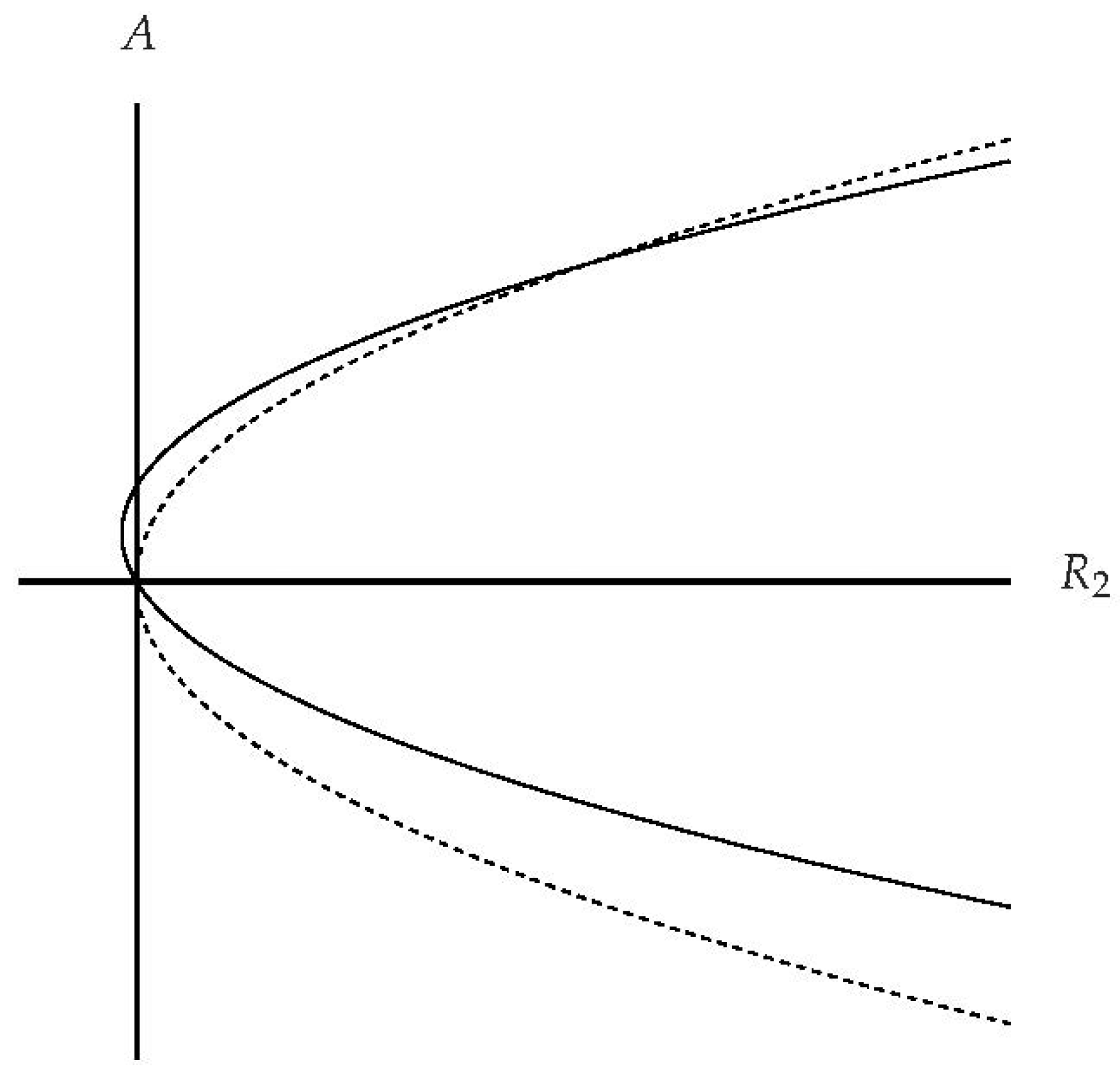
which defines the value of E, the steady equilibrium solution. The plus sign corresponds to the upper branch while the minus sign corresponds to the lower branch; see Figure 1. This solution may be taken as being real, without loss of generality. The bifurcation diagrams corresponding to this solution and that of a single roll solution, e.g., $A=R_2^{1/2}$, $B=C=0$, are both shown in Figure 1. It is well-known that hexagonal solutions bifurcate from the zero solution via a transcritical bifurcation, and subcritical convection occurs at values of $R_2$ that are negative. In this case, hexagonal solutions exist when the following inequality is satisfied,

$$R_2>-\frac{{\alpha }^2}{4(2\mathsf{\Omega }+1)},$$

(33)

as compared with rolls which exist only when $R_2>0$.

We now describe very briefly a straightforward stability analysis of hexagonal solutions. If we perturb the solution given in Equation (32) about $A=B=C=E$ using $A=E+\delta A$ and so on, then we obtain the following linearised perturbation equations for $\delta A$, $\delta B$ and $\delta C$:

$$\delta A_{\tau }=\left[R_2-2E^2(\mathsf{\Omega }+1)\right]\delta A-E^2\left[\delta \overline{A}+\mathsf{\Omega }(\delta B+\delta \overline{B}+\delta C+\delta \overline{C})\right]+\alpha E(\delta B+\delta C),$$

(34)

$$\delta B_{\tau }=\left[R_2-2E^2(\mathsf{\Omega }+1)\right]\delta B-E^2\left[\delta \overline{B}+\mathsf{\Omega }(\delta A+\delta \overline{A}+\delta C+\delta \overline{C})\right]+\alpha E(\delta A+\delta \overline{C}),$$

(35)

$$\delta C_{\tau }=\left[R_2-2E^2(\mathsf{\Omega }+1)\right]\delta C-E^2\left[\delta \overline{C}+\mathsf{\Omega }(\delta A+\delta \overline{A}+\delta B+\delta \overline{B})\right]+\alpha E(\delta A+\delta \overline{B}).$$

(36)

Given their symmetry, these equations may be simplified by setting $\delta B=\delta C$, on noting that it is not possible to set $\delta B=-\delta C$ since then Equations (35) and (36) become inconsistent. Setting both $\delta A$ and $\delta B$ to be imaginary and proportional to $exp\lambda \tau$, where $\lambda$ is real, results in two possible values of $\lambda$, namely, 0 and $-3\alpha E$. Respectively, these mean that the whole of the solution curve is neutrally stable with respect to disturbances in phase, while that part of the lower branch which corresponds to negative values of E is unstable. Repetition of the same procedure with $\delta A$ and $\delta B$ taken to be real yields either

$$\lambda =E\alpha -2(2\mathsf{\Omega }+1)E^2$$

(37)

or

$$\lambda =2(\mathsf{\Omega }-1)E^2-E\alpha .$$

(38)

In Equation (37), $\lambda$ is positive only when positive values of E correspond to points below the turning point on the solution curve, while, in Equation (38), $\lambda$ is positive when

$$E>\frac{\alpha }{\mathsf{\Omega }-1}$$

(39)

or

$$R_2>\frac{(\mathsf{\Omega }+2){\alpha }^2}{{(\mathsf{\Omega }-1)}^2}.$$

(40)

Therefore, we conclude that hexagons exist and are stable in the range

$$-\frac{{\alpha }^2}{4(2\mathsf{\Omega }+1)}\le R_2\le \frac{(\mathsf{\Omega }+2){\alpha }^2}{{(\mathsf{\Omega }-1)}^2},$$

(41)

and for points on the upper branch of the solution curve. Points on the lower branch are always unstable.

5. The Stability of Rolls

We turn now to determining the range of values of $R_2$ within which rolls are stable. Omitting the details, we may perturb about the single roll solution, $A=R_2^{1/2}$, $B=C=0$ in the same way as above. We obtain the perturbation equations,

$$\delta A_{\tau }=-R_2(\delta A+\delta \overline{A}),$$

(42)

$$\delta B_{\tau }=-R_2(\mathsf{\Omega }+1)\delta B+\alpha R_2^{1/2}\delta \overline{C},$$

(43)

$$\delta C_{\tau }=-R_2(\mathsf{\Omega }+1)\delta C+\alpha R_2^{1/2}\delta \overline{B}.$$

(44)

Equation (42) only admits decaying solutions when $\delta A$ is real, and is again neutrally stable to disturbances in phase (i.e., when $\delta A$ is imaginary). Therefore, Equations (43) and (44) must be considered to determine neutral stability. We find that the single roll solution is stable only when

$$R_2>\frac{{\alpha }^2}{{(\mathsf{\Omega }+1)}^2}.$$

(45)

Summarising the above results, we find that hexagons exist when $R_2\ge -151.621$, and rolls exist when $R_2\ge 0$. Hexagons are stable when $R_2\le 26633.8$ and rolls are stable when $R_2\ge 378.693$. Thus, there is an intermediate regime within which both rolls and hexagons are stable to infinitesimal disturbances. Although we do not prove it here, there is a mixed mode branch of unstable solutions which bifurcates away from the roll branch at $R_2=378.693$ and then joins the branch of hexagonal solutions at $R_2=26633.8$ as a subcritical bifurcation.

6. The Effect of Forchheimer Terms on Hexagonal Cells

We now consider the additional effect of form drag, as modelled by the Forchheimer terms. Following Rees [17], the non-dimensional equations that govern those cases where the quadratic Forchheimer terms are significant are given by

$${\displaystyle \frac{\partial u}{\partial x}}+{\displaystyle \frac{\partial v}{\partial y}}+{\displaystyle \frac{\partial w}{\partial z}}=0,$$

(46)

$$u(1+G|\overrightarrow{u}\left|\right)=-{\displaystyle \frac{\partial p}{\partial x}},$$

(47)

$$v(1+G|\overrightarrow{u}\left|\right)=-{\displaystyle \frac{\partial p}{\partial y}},$$

(48)

$$w(1+G|\overrightarrow{u}\left|\right)=-{\displaystyle \frac{\partial p}{\partial z}}+\mathrm{Ra}\theta ,$$

(49)

$${\displaystyle \frac{\partial \theta }{\partial t}}+u{\displaystyle \frac{\partial \theta }{\partial x}}+v{\displaystyle \frac{\partial \theta }{\partial y}}+w{\displaystyle \frac{\partial \theta }{\partial z}}={\displaystyle \frac{{\partial }^2\theta }{\partial x^2}}+{\displaystyle \frac{{\partial }^2\theta }{\partial y^2}}+{\displaystyle \frac{{\partial }^2\theta }{\partial z^2}}+ϵ(u^2+v^2+w^2),$$

(50)

where

$${\displaystyle G=\frac{\tilde{K}k}{\mu d{C}_p}.}$$

(51)

The constant $\tilde{K}$, which appears in Equation (51), is quoted by many papers to be given by Ergun’s relation, $\tilde{K}=1.75L/150(1-\mathrm{\Phi })$, (Nield and Bejan [3]), where L is a lengthscale associated with the microstructure of the medium, and $\mathrm{\Phi }$ is the effective porosity. Again, following Rees [17], we need to rescale G according to

$$G=ϵG^{*},$$

(52)

so that form drag effects are felt at $O\left({ϵ}^3\right)$, rather than at $O\left({ϵ}^2\right)$. The value, $G^{*}$, is termed the Forchheimer parameter.

The expansion proceeds as before and with exactly the same solutions up to $O\left({ϵ}^2\right)$. At $O\left({ϵ}^3\right)$, the presence of form drag yields further inhomogeneous terms that must be included into the solvability condition. The $O\left({ϵ}^3\right)$ equations are now given by

$${\nabla }^2{p}_3-R_0{\displaystyle \frac{\partial {\theta }_3}{\partial z}}=R_2{\displaystyle \frac{\partial {\theta }_1}{\partial z}}-G^{*}\left[u_1{\displaystyle \frac{\partial q_1}{\partial x}}+v_1{\displaystyle \frac{\partial q_1}{\partial y}}+w_1{\displaystyle \frac{\partial q_1}{\partial z}}\right],$$

(53)

$$\begin{array}{cc}\hfill {\nabla }^2{\theta }_3+R_0{\theta }_3-{\displaystyle \frac{\partial p_3}{\partial z}}& =R_0\left({\theta }_1{\displaystyle \frac{\partial {\theta }_2}{\partial z}}+{\theta }_2{\displaystyle \frac{\partial {\theta }_1}{\partial z}}\right)-\nabla p_1.\nabla {\theta }_2-\nabla p_2.\nabla {\theta }_1-R_2{\theta }_1+\frac{1}{2}{\displaystyle \frac{\partial {\theta }_1}{\partial \tau }}\hfill \\ & -{\left({\displaystyle \frac{\partial p_1}{\partial x}}\right)}^2-{\left({\displaystyle \frac{\partial p_1}{\partial y}}\right)}^2-{\left({\displaystyle \frac{\partial p_1}{\partial z}}-R_0{\theta }_1\right)}^2.\hfill \end{array}$$

(54)

In Equations (53) and (54), the values $u_1$, $v_1$ and $w_1$ are the velocities corresponding to the $O\left(ϵ\right)$ pressure distribution, $p_1$, and the value $q_1$ is the $O\left(ϵ\right)$ velocity,

$$q_1^2=u_1^2+v_1^2+w_1^2={\left({\displaystyle \frac{\partial p_1}{\partial x}}\right)}^2+{\left({\displaystyle \frac{\partial p_1}{\partial y}}\right)}^2+{\left({\displaystyle \frac{\partial p_1}{\partial z}}-R_0{\theta }_1\right)}^2.$$

(55)

The separate application of the solvability condition (26) for all three roll directions now yields the following amplitude equations:

$$A_{\tau }=R_{2}A-A^2\overline{A}-\mathsf{\Omega }A(B\overline{B}+C\overline{C})+\alpha BC-\mathcal{F}(A,B,C)G^{*}A,$$

(56)

$$B_{\tau }=R_{2}B-B^2\overline{B}-\mathsf{\Omega }B(A\overline{A}+C\overline{C})+\alpha A\overline{C}-\mathcal{F}(A,B,C)G^{*}B,$$

(57)

$$C_{\tau }=R_{2}C-C^2\overline{C}-\mathsf{\Omega }C(A\overline{A}+B\overline{B})+\alpha A\overline{B}-\mathcal{F}(A,B,C)G^{*}C.$$

(58)

The final coefficient in these amplitude equations is given by

$$\mathcal{F}(A,B,C)={\displaystyle \frac{\sqrt{3}{\pi }^2}{8}}{\int }_0^1{\int }_0^{4/\sqrt{3}}{\int }_0^4\widehat{p}\left[u_1{\displaystyle \frac{\partial q_1}{\partial x}}+v_1{\displaystyle \frac{\partial q_1}{\partial y}}+w_1{\displaystyle \frac{\partial q_1}{\partial z}}\right]dxdydz.$$

(59)

The value of this integral depends on the relative magnitudes of A, B and C, and cannot be evaluated analytically. However, for steady rolls and hexagons, we have

$$\mathrm{rolls:}A=E,B=C=0\Rightarrow \mathcal{F}=61.3127\left|E\right|,$$

(60)

$$\mathrm{hexagons:}A=B=C=E\Rightarrow \mathcal{F}=119.4882\left|E\right|.$$

(61)

The numerical value given in Equation (60) is consistent with that given in Rees [17]. If one were to wish to follow the time-evolution of A, B and C, then it would be necessary to evaluate $\mathcal{F}$ at every timestep.

We may now consider the effect of the Forchheimer terms on the amplitude on hexagonal convection. If we set A, B and C to all be equal to E, which is real, and assume that the flow is steady, then E satisfies the equation

$$R_{2}E-(2\mathsf{\Omega }+1)E^3+\alpha E^2-\gamma \left|E\right|E=0,$$

(62)

where we have set $\gamma =119.4882G^{*}$ for simplicity of presentation. In this rather unusual amplitude equation, it is clear that $E=0$ remains a possible solution, but the nonzero solutions now satisfy

$$R_2=(2\mathsf{\Omega }+1)E^2-\alpha E+\gamma \left|E\right|.$$

(63)

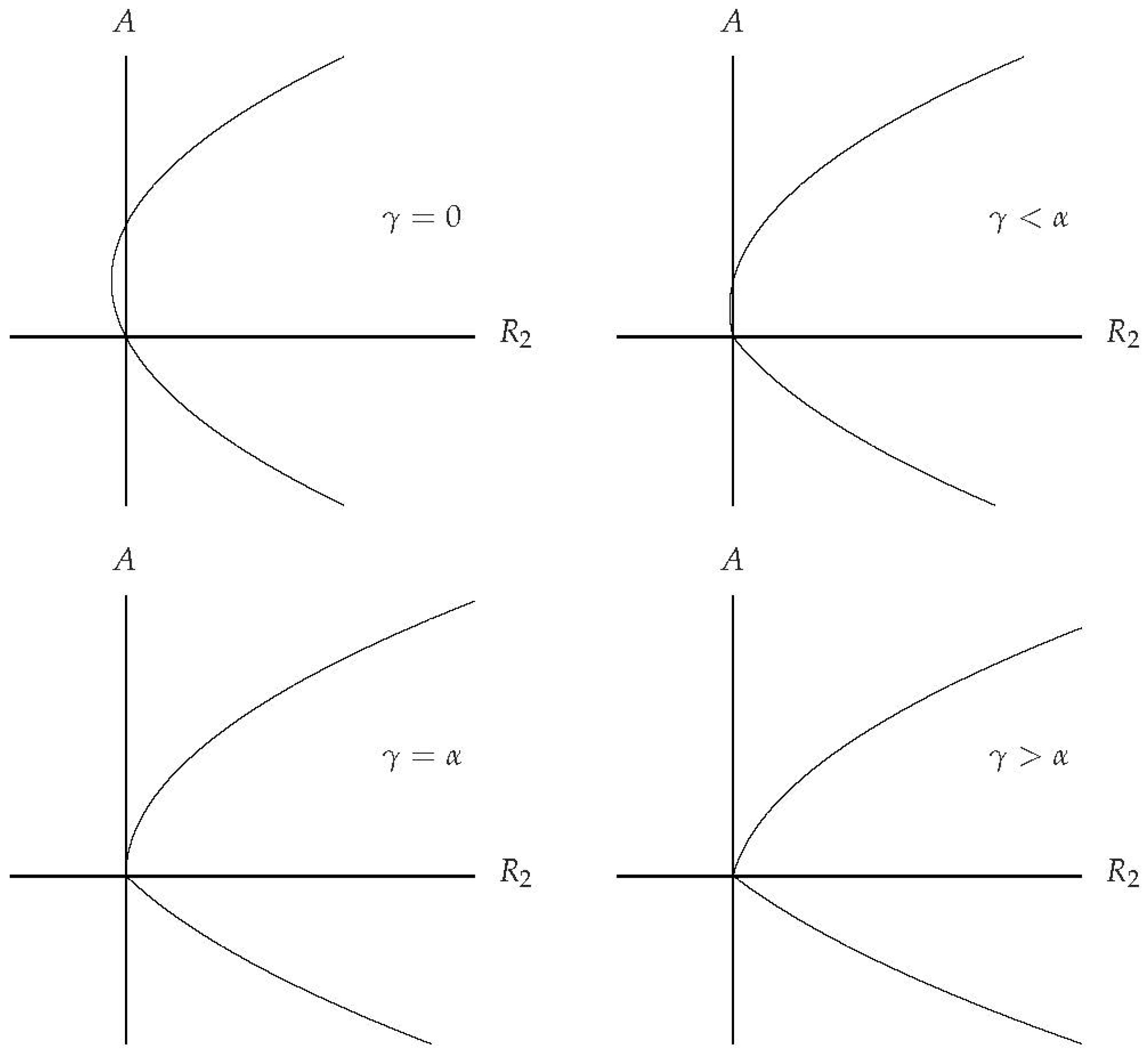
The solution curves for E fall into four different cases depending on the magnitudes of $\gamma (>0)$ and $\alpha$, and these are sketched in Figure 2.

When $\gamma =0$ form drag effects are absent, the flows considered earlier apply. When $0<\gamma <\alpha$, there remains a subcritical flow on the upper branch of the solution curve, but the degree of subcriticality has now been reduced. In this range of values of $\gamma$, it is shown easily that the smallest value of $R_2$ on the upper solution branch is given by

$$R_2=-\frac{1}{4}\frac{{(\alpha -\gamma )}^2}{2\mathsf{\Omega }+1},$$

(64)

at which point the amplitude of convection is given by

$$E=\frac{1}{2}\frac{\alpha -\gamma }{2\mathsf{\Omega }+1}.$$

(65)

In this range of values of $\gamma$, the lower branch becomes weaker in the sense that $\left|E\right|$ decreases when $\gamma$ increases for any chosen value of $R_2$; this is a consequence of form drag reducing the efficacy of buoyancy forces to cause flow. There is also a discontinuous change of slope of the lower branch at $R_2=0$, where $\left|E\right|=E$ changes to $\left|E\right|=-E$.

At the point where $\gamma =\alpha$, the upper branch becomes a parabola, which is characteristic of a standard supercritical pitchfork bifurcation. Therefore, subcritical flow does not exist when $G^{*}\ge \alpha /119.4882$, or, equivalently, when $Ge$ is small:

$$G\ge 4Ge/119.4882\pi .$$

(66)

As $\gamma$ continues to increase above $\alpha$, the amplitudes of convection at any chosen positive value of $R_2$ continues to decrease, and the onset of convection is via an asymmetric sharp-nosed bifurcation. The lower branch remains unstable for small disturbances while the upper branch is stable initially as $R_2$ increases above zero. The equivalent situation for rolls, given in [13], is that the bifurcation is also sharp-nosed, but the bifurcation diagram remains symmetric.

7. Effect of the Forchheimer Terms on Stability

Finally, we present information on how the presence of form-drag affects the stability boundaries for hexagons and rolls. We omit all of the details and find that hexagons are unstable when

$$R_2>\frac{{\alpha }^2}{{(\mathsf{\Omega }-1)}^2}\left[\mathsf{\Omega }+2+119.4882G^{*}\right],$$

(67)

while rolls are stable when

$$R_2>\frac{{\alpha }^2}{{(\mathsf{\Omega }+1)}^2}+61.3126G^{*}\frac{\alpha }{\mathsf{\Omega }-1}.$$

(68)

Thus, hexagons increase and rolls decrease their respective ranges of stability when form drag becomes increasingly important.

8. Conclusions

We have sought to determine the combined effect of viscous dissipation and form drag on Darcy–Bénard convection. Viscous dissipation serves to cause the stable pattern of convection to change from rolls to hexagons for a range of values of the Darcy–Rayleigh number, which includes the critical value, $\mathrm{Ra}=4{\pi }^2$, or, equivalently, $R_2=0$.

We have determined the range of stability of these patterns and compared them with that for rolls, which eventually re-emerge as the stable pattern as the Darcy–Rayleigh number increases. We find that form drag alters the shape of the solution curves to such an extent that, when it is sufficiently strong, there is no longer any subcritical convection, which is the ubiquitous characteristic of hexagonal patterns. Form drag also increases the size of the region within which hexagons are stable and that region within which rolls are unstable.

It is in the nature of weakly nonlinear theory that the phenomena it predicts take place close to the onset of convection. It provides an accurate indicator of the qualitative behaviour that will arise when governing parameters take larger values. In the present paper, we have considered both the viscous dissipation and form drag to be weak, and therefore the detailed behaviour of hexagonal cells which have been described take place asymptotically close to $\mathrm{Ra}=4{\pi }^2$. Should the Gebhart number not be asymptotically small, then hexagonal convection will arise at values of the Darcy–Rayleigh number, which are at $O\left(1\right)$ distances from the critical value, and therefore they will be seen easily in practice. In addition, if form drag effects are also strong, then the loss of subcriticality shown in Figure 2 will also be visible practically. The message from our analysis is that there will be $O\left(1\right)$ values of both the Gebhart and Forchheimer parameters that also obey the qualitative behaviours which we have described here.

It is also worth stating that other agencies will alter the symmetry of the basic temperature field to cause hexagons to arise preferentially—this includes a temperature-dependent thermal diffusivity and weak vertical throughflow as first considered by Wooding [18] and Sutton [19]. However, the manner in which the weakly nonlinear theory progresses suggests that any changes to the present analysis will only be quantitative, and, in these cases, the general qualitative behaviour will be identical to that presented here.

Finally, we note that Rebhi et al. [20], who have studied the onset and nonlinear development of double-diffusive convection in a porous cavity, have identified regimes within which convection is subcritical in the sense that it is possible for nonlinear flow to exist at values of the Darcy–Rayleigh number that are below that given by linearised stability theory. The chief interest of this paper in the present context is the observation that an increasingly strong form-drag also removes the subcriticality of the cavity flows. It is difficult to know whether this qualitative similarity between two very different flows has a great significance, for the mechanisms which cause subcritical convection are quite different in the respective cases.