CFD Analyses and Experiments in a PAT Modeling: Pressure Variation and System Efficiency


Abstract
:1. Introduction
2. Numerical and Experimental Procedure
2.1. PAT Numerical Model
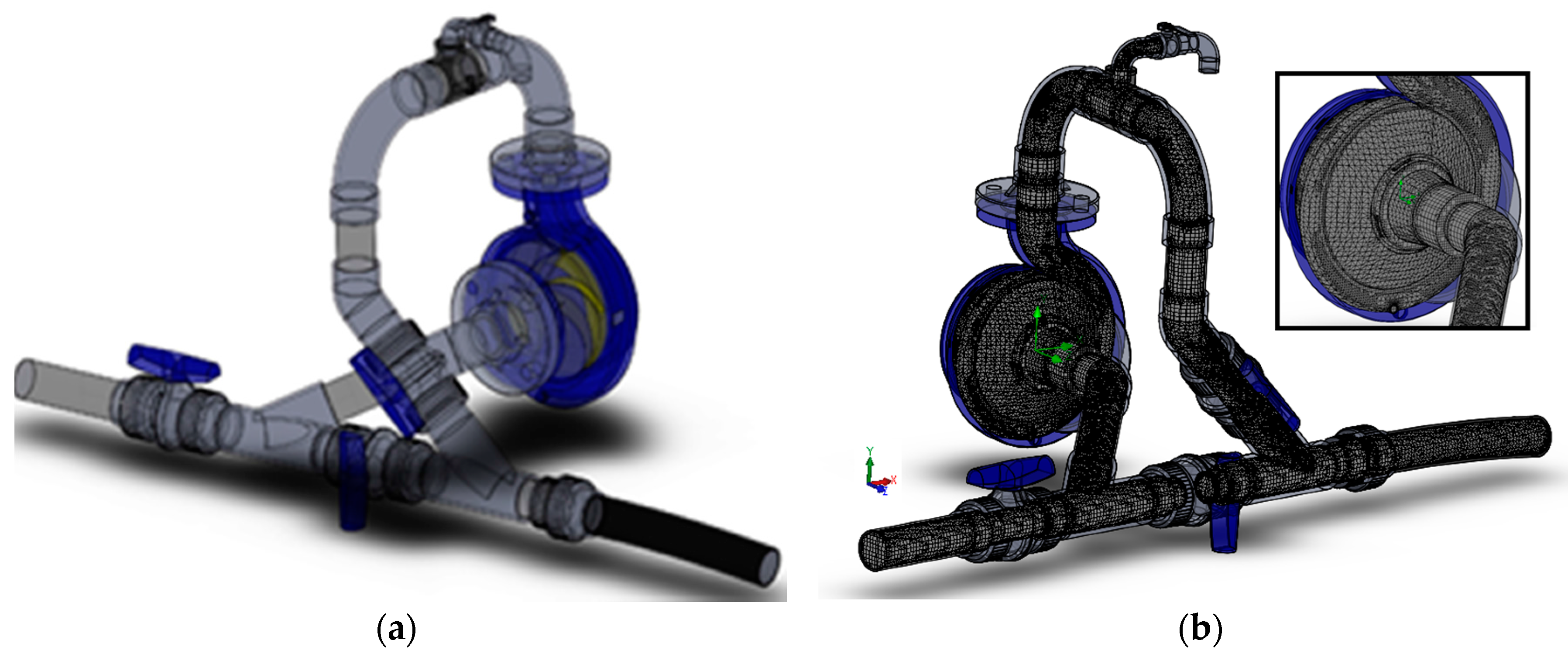
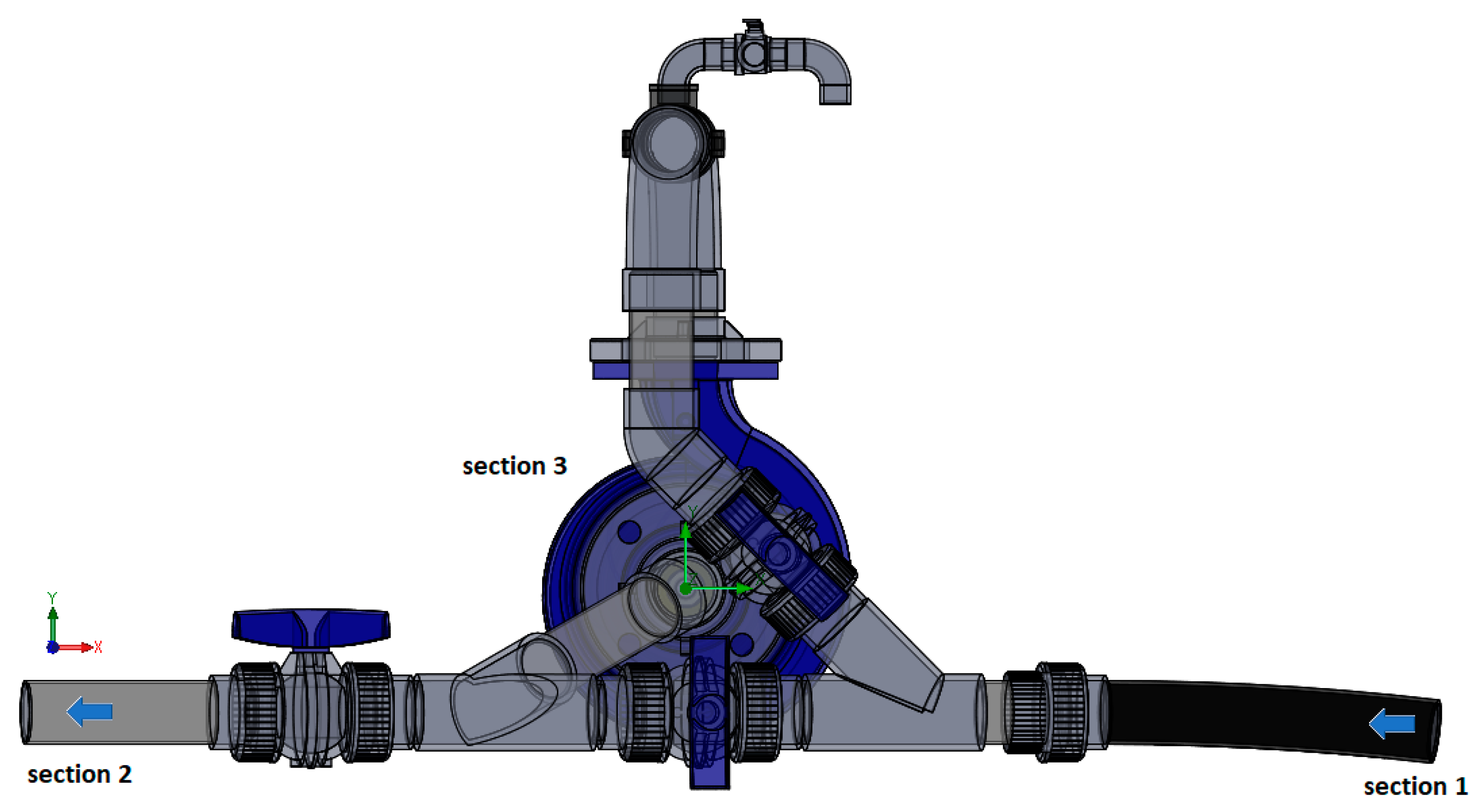
2.1.1. Model Description and Mesh
2.1.2. Boundary Conditions
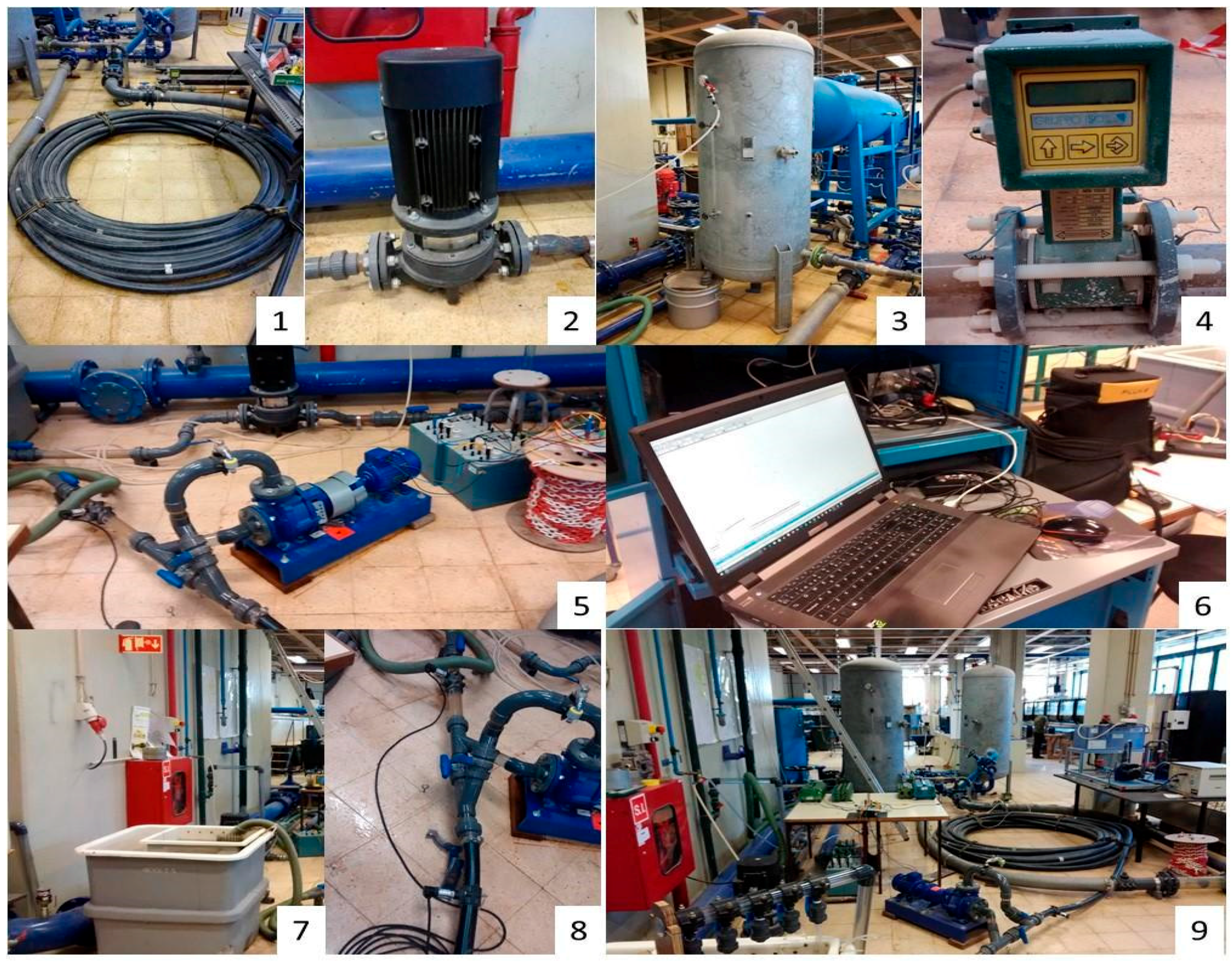
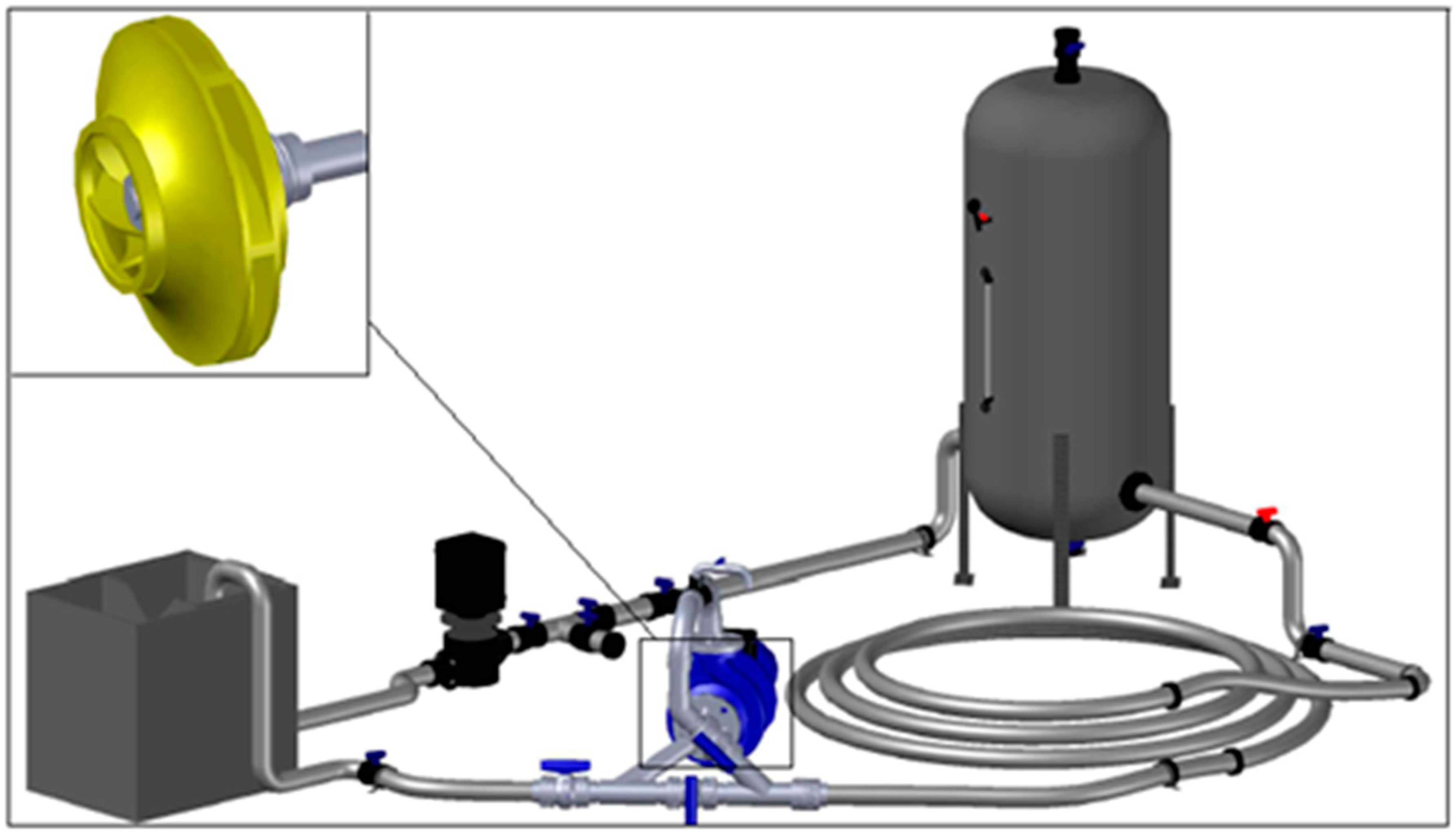
2.2. PAT Experimental Tests
3. Results and Discussion
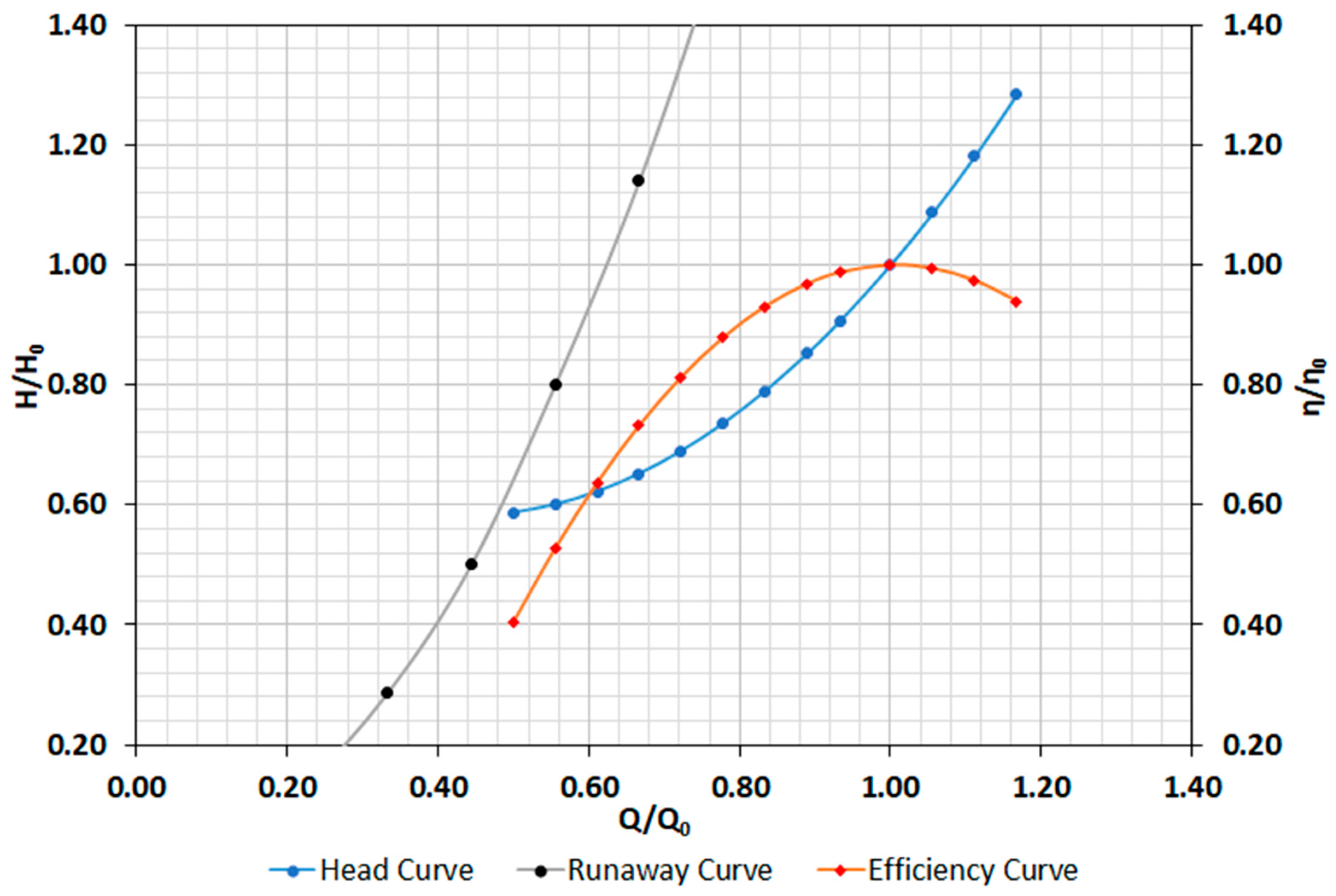
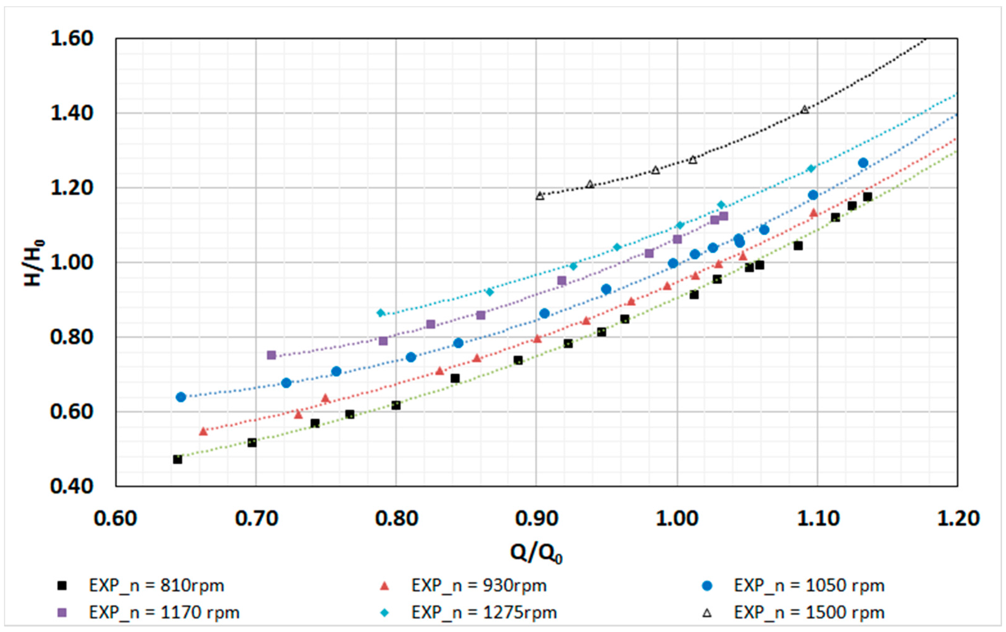
3.1. PAT Characteristics
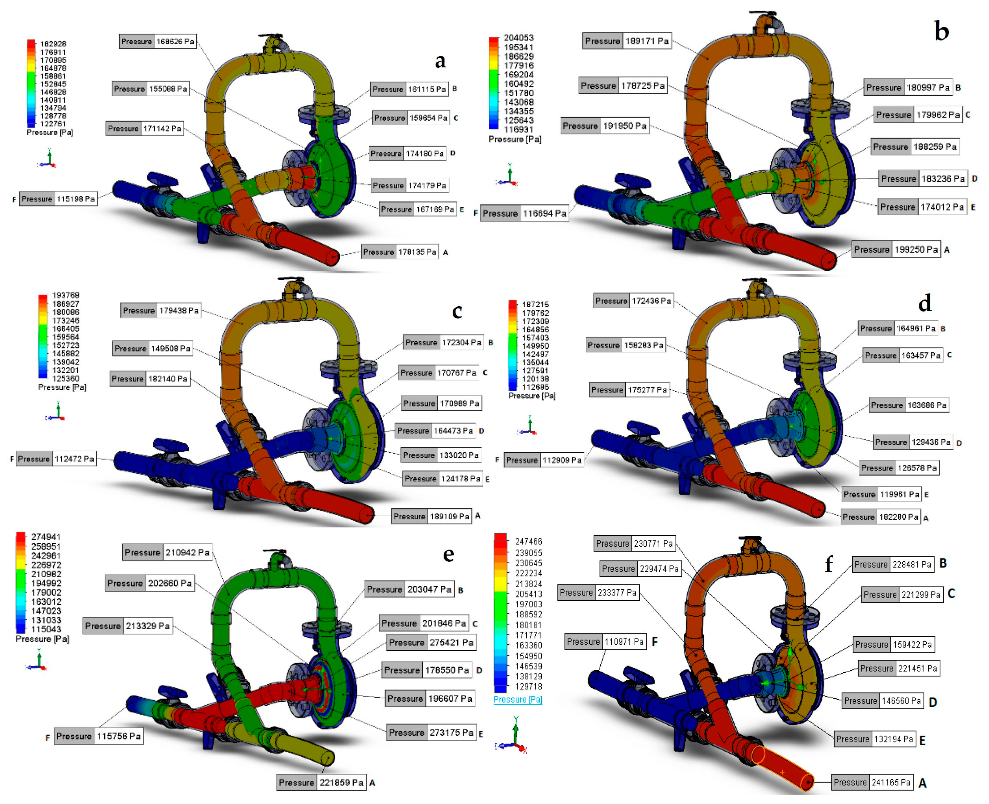
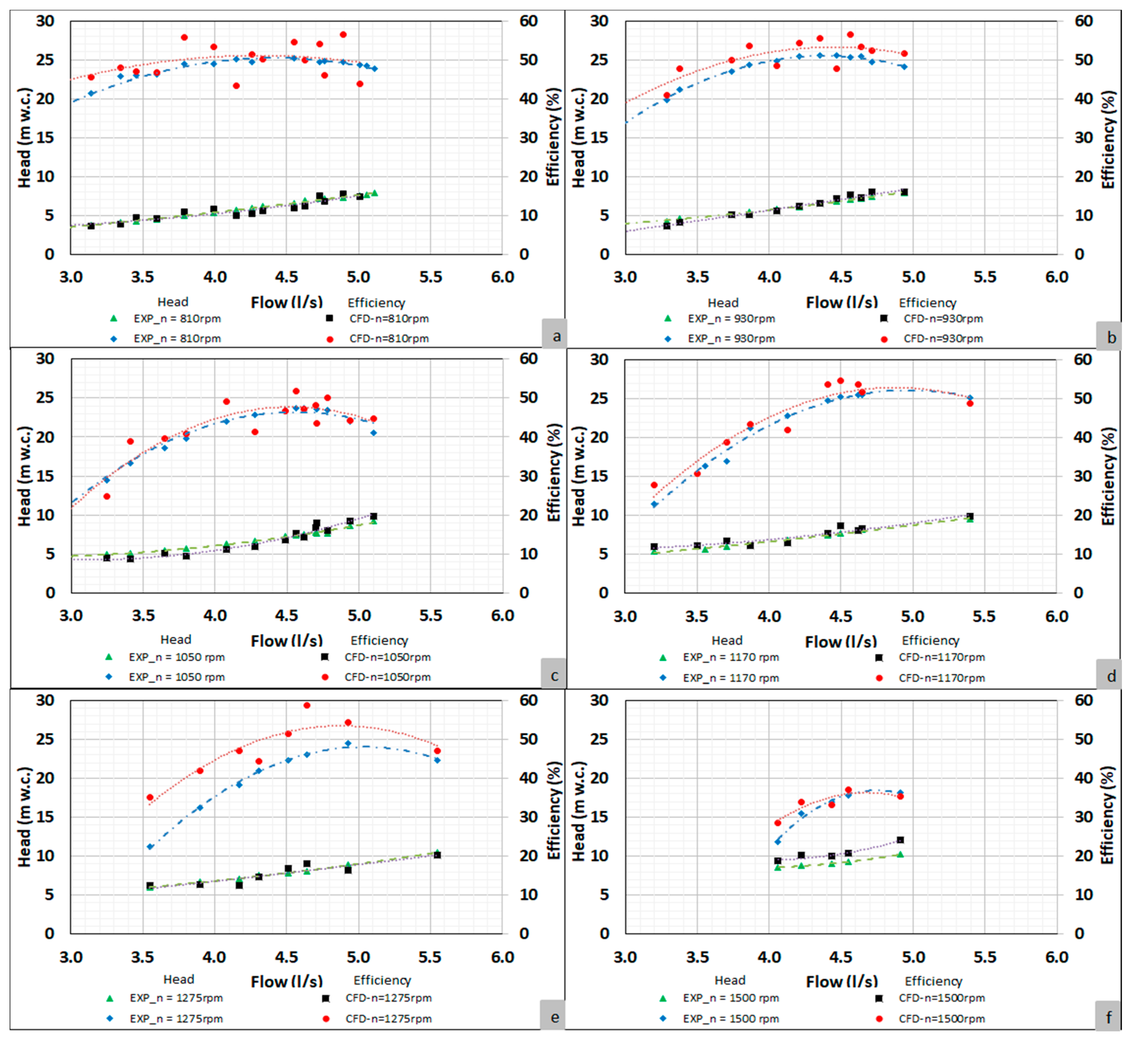
3.2. CFD and Experiments
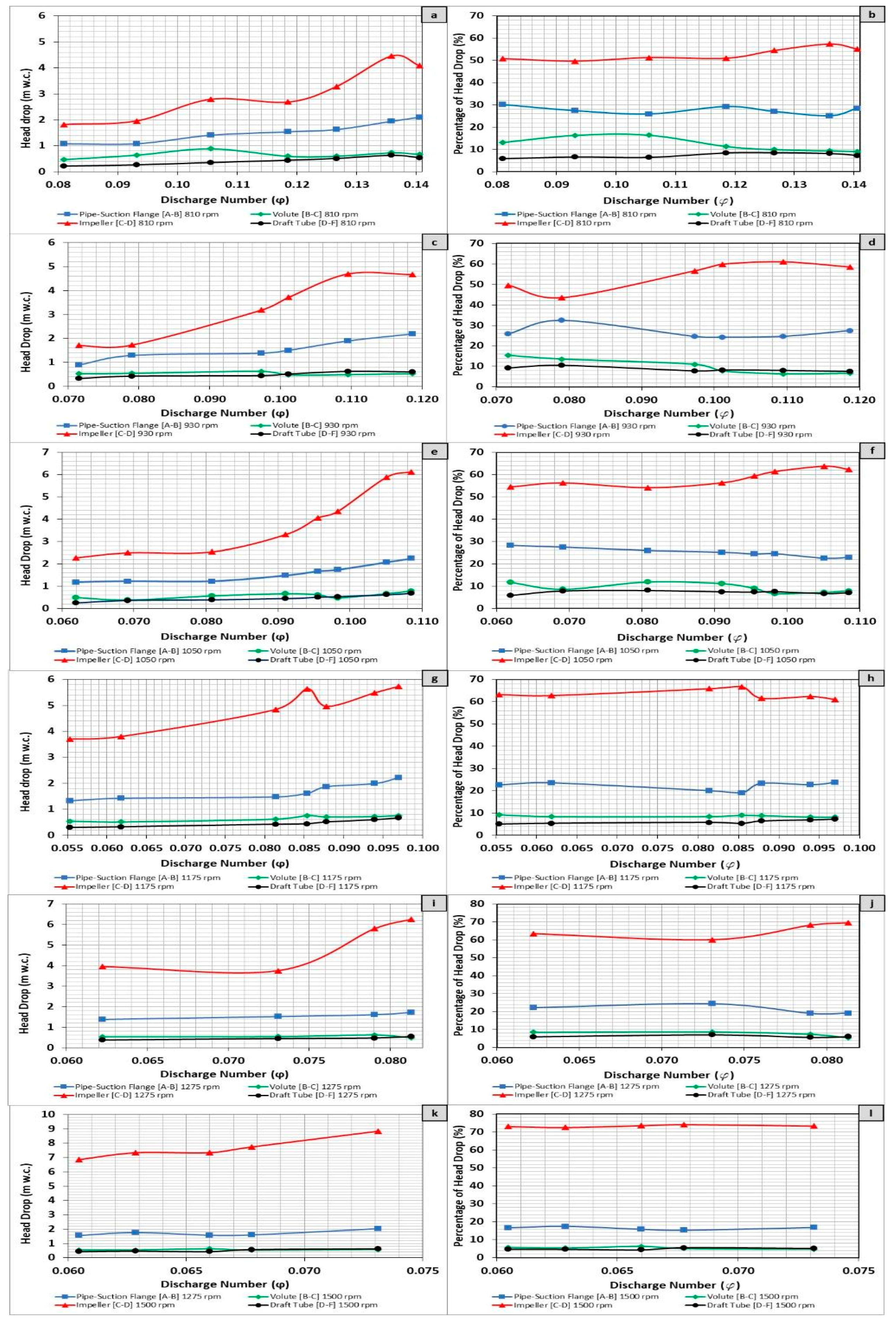
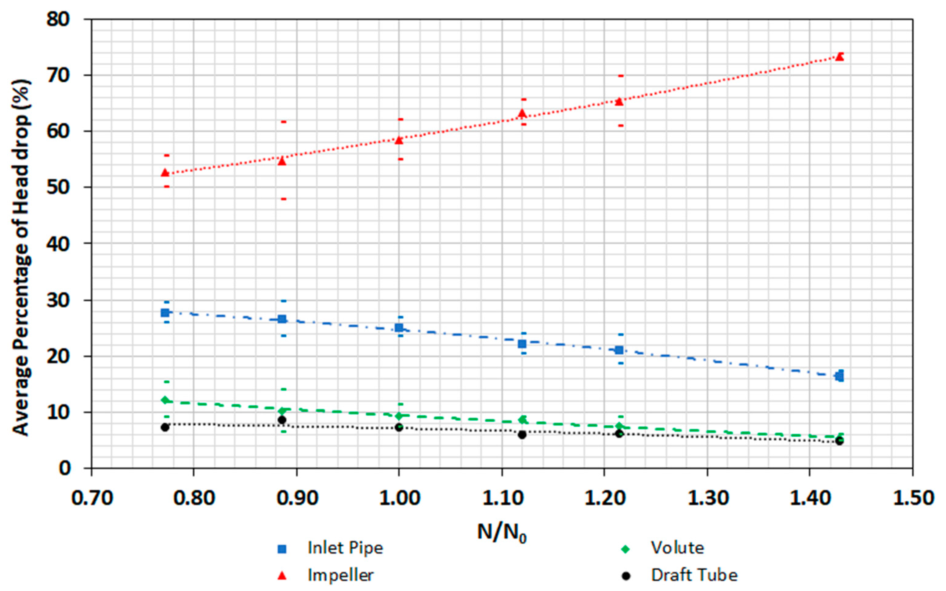
3.3. Head Drop Estimation
4. Conclusions
Acknowledgments
Author Contributions
Conflicts of Interest
Abbreviations
| BEP | Best Efficiency Point |
| CFD | Computational Fluids Dynamics |
| FVM | Finite Volume Methods |
| PATs | Pumps working as Turbines |
| SAR | Solution Adaptive Refinement |
| SIMPLE | Semi Implicit Method for Pressure-Linked Equations |
| VOS | Variable Operation Strategy |
References
- Cabrera, E.; Cobacho, R.; Soriano, J. Towards an energy labelling of pressurized water networks. Procedia Eng. 2014, 70, 209–217. [Google Scholar] [CrossRef]
- Tucciarelli, T.; Criminisi, A.; Termini, D. Leak analysis in pipeline systems by means of optimal valve regulation. J. Hydraul. Eng. 1999, 125, 277–285. [Google Scholar] [CrossRef]
- Lansey, K.E.; Mays, L.W. Optimization model for water distribution system design. J. Hydraul. Eng. 1990, 115, 1401–1418. [Google Scholar] [CrossRef]
- Araujo, L.; Ramos, H.; Coelho, S. Pressure control for leakage minimisation in water distribution systems management. Water Resour. Manag. 2006, 20, 133–149. [Google Scholar] [CrossRef]
- Ramos, H.; Borga, A. Pumps as turbines: An unconventional solution to energy production. Urban. Water. 1999, 1, 261–263. [Google Scholar] [CrossRef]
- Pérez-Sánchez, M.; Sánchez-Romero, F.; Ramos, H.; López-Jiménez, P. Energy recovery in existing water networks: Towards greater sustainability. Water 2017, 9, 97. [Google Scholar] [CrossRef]
- Yang, S.S.; Derakhshan, S.; Kong, F.Y. Theoretical, numerical and experimental prediction of pump as turbine performance. Renew. Energy 2012, 48, 507–513. [Google Scholar] [CrossRef]
- Nautiyal, H.; Varun, K.A. Reverse running pumps analytical, experimental and computational study: A review. Renew. Sustain. Energy Rev. 2010, 14, 2059–2067. [Google Scholar] [CrossRef]
- Carravetta, A.; Del Giudice, G.; Fecarotta, O.; Ramos, H. PAT design strategy for energy recovery in water distribution networks by electrical regulation. Energies 2013, 6, 411–424. [Google Scholar] [CrossRef]
- Fecarotta, O.; Carravetta, A.; Ramos, H.M.; Martino, R. An improved affinity model to enhance variable operating strategy for pumps used as turbines. J. Hydraul. Res. 2016, 54, 332–341. [Google Scholar] [CrossRef]
- Pérez-Sánchez, M. Methodology for energy efficiency analysis in pressurized irrigation networks. Ph.D. Thesis, Universitat Politècnica Valencia, València, Spain, 2017. [Google Scholar]
- López-Jiménez, P.A.; Escudero-González, J.; Montoya Martínez, T.; Fajardo Montañana, V.; Gualtieri, C. Application of CFD methods to an anaerobic digester: The case of Ontinyent WWTP, Valencia, Spain. J. Water Process. Eng. 2015, 7, 131–140. [Google Scholar] [CrossRef]
- Ramos, H.M.; Simão, M.; Borga, A. Experiments and CFD analyses for a new reaction microhydro propeller with five blades. J. Energy Eng. 2013, 139, 109–117. [Google Scholar] [CrossRef]
- Simao, M.; Mora-Rodriguez, J.; Ramos, H.M. Computational dynamic models and experiments in the fluid-structure interaction of pipe systems. Can. J. Civ. Eng. 2016, 43, 60–72. [Google Scholar] [CrossRef]
- Simão, M.; Ramos, H.M. Hydrodynamic and performance of low power turbines: Conception, modelling and experimental tests. Int. J. Energy Environ. 2010, 1, 431–444. [Google Scholar]
- Nautiyal, H.; Nautiyal, H.; Varun, V.; Kumar, A.; Yadav, S.Y.S. Experimental investigation of centrifugal pump working as turbine for small hydropower systems. Energy Sci. Technol. 2011, 1, 79–86. [Google Scholar] [CrossRef]
- Derakhshan, S.; Nourbakhsh, A. Experimental study of characteristic curves of centrifugal pumps working as turbines in different specific speeds. Exp. Therm. Fluid Sci. 2008, 32, 800–807. [Google Scholar] [CrossRef]
- Yang, S.S.; Kong, F.Y.; Chen, H.; Su, H.S. Effects of blade wrap angle influencing a pump as turbine. J. Fluids Eng. 2012, 134, 061102. [Google Scholar] [CrossRef]
- Griffini, D.; Insinna, M.; Salvadori, S.; Barucci, A.; Cosi, F.; Pelli, S.; Righini, G.C. On the CFD analysis of a stratified Taylor-Couette system dedicated to the fabrication of nanosensors. Fluids 2017, 2, 8. [Google Scholar] [CrossRef]
- Mentor Graphics Corporation. FloEFD Technical Reference; Mentor Graphics Corporation: Wilsonville, OR, USA, 2011. [Google Scholar]
- Mentor Graphics Corporation. Flow Simulation—Technical Reference; Solid Works 2011; E.U.A., Ed.; Mentor Graphics Corporation: Wilsonville, OR, USA, 2011. [Google Scholar]
- Guidelines for Design of Small Hydropower Plants; Ramos, H. (Ed.) WREAN (Western Regional Energy Agency and Network) and DED (Department of Economic Development—Energy Division): Belfast, Northern Ireland, UK, 2000.


| Rotational Speed (rpm) | Refinement Level | Fluid Cells | Number of Iterations | Tolerance | Simulation Time (s) |
|---|---|---|---|---|---|
| 810 | 2 | 100631 | 430 | 0.001 | 4402 |
| 930 | 2 | 100651 | 449 | 4416 | |
| 1050 | 2 | 100691 | 459 | 4423 | |
| 1170 | 4 | 101936 | 677 | 5472 | |
| 1275 | 5 | 102274 | 961 | 8225 | |
| 1500 | 4 | 101936 | 477 | 4973 |
| N/N0 | Mean Square Error | |
|---|---|---|
| Head | Efficiency | |
| 0.77 | 0.0197 | 0.0262 |
| 0.89 | 0.0266 | 0.0241 |
| 1.00 | 0.0264 | 0.0233 |
| 1.12 | 0.0236 | 0.0305 |
| 1.21 | 0.0268 | 0.0944 |
| 1.43 | 0.0869 | 0.0966 |
| N (rpm) | 810 | N/N0 | 0.77 | N (rpm) | 930 | N/N0 | 0.89 | ||||||
| Q (L/s) | Head values (m w.c.) | Q (L/s) | H (m w.c.) | ||||||||||
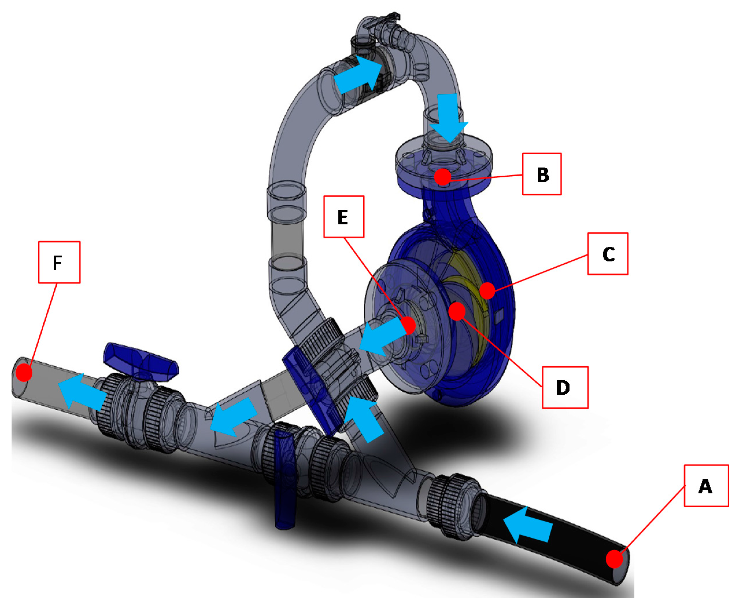
| A | B | C | D | E | F | A | B | C | D | E | F | ||
| 2.90 | 4.67 | 3.59 | 3.12 | 1.30 | 1.28 | 1.09 | 2.98 | 4.39 | 3.50 | 2.97 | 1.26 | 1.23 | 0.94 |
| 3.34 | 5.01 | 3.93 | 3.29 | 1.33 | 1.25 | 1.07 | 3.29 | 5.10 | 3.81 | 3.27 | 1.54 | 1.53 | 1.12 |
| 3.79 | 5.78 | 4.37 | 3.48 | 0.69 | 0.68 | 0.34 | 4.05 | 6.78 | 5.40 | 4.78 | 1.59 | 1.56 | 1.15 |
| 4.26 | 6.18 | 4.64 | 4.04 | 1.36 | 1.33 | 0.92 | 4.21 | 7.11 | 5.61 | 5.13 | 1.41 | 1.38 | 0.90 |
| 4.55 | 7.18 | 5.55 | 4.95 | 1.67 | 1.51 | 1.16 | 4.56 | 8.89 | 6.99 | 6.50 | 1.80 | 1.78 | 1.18 |
| 4.89 | 8.96 | 7.01 | 6.28 | 1.82 | 1.77 | 1.19 | 4.94 | 8.99 | 6.79 | 6.26 | 1.59 | 1.52 | 0.99 |
| 5.06 | 8.19 | 6.08 | 5.41 | 1.33 | 1.30 | 0.79 | |||||||
| N (rpm) | 1050 | N/N0 | 1.00 | N (rpm) | 1175 | N/N0 | 1.12 | ||||||
| Q (L/s) | H (m w.c.) | Q (L/s) | H (m w.c.) | ||||||||||
| A | B | C | D | E | F | A | B | C | D | E | F | ||
| 2.91 | 5.49 | 4.31 | 3.82 | 1.54 | 1.51 | 1.30 | 2.91 | 6.66 | 5.34 | 4.80 | 1.10 | 1.08 | 0.81 |
| 3.25 | 5.61 | 4.39 | 4.01 | 1.51 | 1.49 | 1.16 | 3.25 | 7.49 | 6.07 | 5.56 | 1.76 | 1.74 | 1.44 |
| 3.80 | 4.94 | 3.72 | 3.16 | 0.62 | 0.61 | 0.24 | 4.28 | 8.33 | 6.86 | 6.24 | 1.40 | 1.36 | 0.98 |
| 4.28 | 7.04 | 5.56 | 4.91 | 1.59 | 1.54 | 1.15 | 4.49 | 9.61 | 8.00 | 7.24 | 1.60 | 1.56 | 1.16 |
| 4.49 | 7.92 | 6.25 | 5.64 | 1.58 | 1.55 | 1.08 | 4.62 | 9.14 | 7.27 | 6.56 | 1.60 | 1.56 | 1.09 |
| 4.62 | 8.50 | 6.76 | 6.29 | 1.94 | 1.88 | 1.41 | 4.94 | 9.94 | 7.95 | 7.23 | 1.75 | 1.74 | 1.15 |
| 5.10 | 10.73 | 8.48 | 7.71 | 1.58 | 1.55 | 0.89 | |||||||
| N (rpm) | 1275 | N/N0 | 1.21 | N (rpm) | 1500 | N/N0 | 1.43 | ||||||
| Q (L/s) | H (m w.c.) | Q (L/s) | H (m w.c.) | ||||||||||
| A | B | C | D | E | F | A | B | C | D | E | F | ||
| 3.55 | 7.10 | 5.72 | 5.19 | 1.24 | 1.23 | 0.87 | 4.06 | 10.47 | 8.91 | 8.38 | 1.53 | 1.51 | 1.09 |
| 4.17 | 7.48 | 5.96 | 5.42 | 1.67 | 1.65 | 1.23 | 4.22 | 11.85 | 10.09 | 9.55 | 2.22 | 2.20 | 1.75 |
| 4.51 | 9.94 | 8.33 | 7.71 | 1.91 | 1.89 | 1.44 | 4.43 | 11.42 | 9.84 | 9.22 | 1.89 | 1.87 | 1.45 |
| 4.64 | 10.46 | 8.74 | 8.26 | 2.00 | 1.97 | 1.46 | 4.55 | 11.39 | 9.79 | 9.26 | 1.53 | 1.45 | 0.96 |
© 2017 by the authors. Licensee MDPI, Basel, Switzerland. This article is an open access article distributed under the terms and conditions of the Creative Commons Attribution (CC BY) license (http://creativecommons.org/licenses/by/4.0/).
Share and Cite
Pérez-Sánchez, M.; Simão, M.; López-Jiménez, P.A.; Ramos, H.M. CFD Analyses and Experiments in a PAT Modeling: Pressure Variation and System Efficiency. Fluids 2017, 2, 51. https://doi.org/10.3390/fluids2040051
Pérez-Sánchez M, Simão M, López-Jiménez PA, Ramos HM. CFD Analyses and Experiments in a PAT Modeling: Pressure Variation and System Efficiency. Fluids. 2017; 2(4):51. https://doi.org/10.3390/fluids2040051
Chicago/Turabian StylePérez-Sánchez, Modesto, Mariana Simão, P. Amparo López-Jiménez, and Helena M. Ramos. 2017. "CFD Analyses and Experiments in a PAT Modeling: Pressure Variation and System Efficiency" Fluids 2, no. 4: 51. https://doi.org/10.3390/fluids2040051
APA StylePérez-Sánchez, M., Simão, M., López-Jiménez, P. A., & Ramos, H. M. (2017). CFD Analyses and Experiments in a PAT Modeling: Pressure Variation and System Efficiency. Fluids, 2(4), 51. https://doi.org/10.3390/fluids2040051