A Finite Element Method for Incompressible Fluid Flow in a Noninertial Frame of Reference and a Numerical Study of Circular Couette Flow with Varying Angular Speed

Abstract

In this work, we develop a numerical strategy for analyzing the flows of an incompressible fluid in the gap between an arbitrarily shaped inner boundary that rotates inside a circular outer boundary. Such flows occur very commonly in turbomachinery applications. The numerical strategy is based on a noninertial frame of reference that is fixed to the rotating inner boundary so that Coriolis and angular acceleration effects have to be accounted for in its development. Since this strategy is based on a fixed mesh, it is much more economical and accurate than a general arbitrary Eulerian–Lagrangian strategy, which would typically require remeshing. In addition, we also conduct a numerical study for circular Couette flow with varying angular speed of the inner cylinder in an inertial frame of reference; such a study may prove useful in validating a theoretical stability analysis which currently seems to have been carried out only for the case of constant angular speed.

1. Introduction

This work develops a velocity-pressure integrated finite element formulation in a non-inertial frame for the general case of three-dimensional incompressible fluid flow without any simplifying assumptions such as potential flow. Most of the existing work has focused on inertial frame formulations. Kim [1] presented a velocity-pressure integrated mixed interpolation method for the analysis of fluid flows. Kim and Decker [2] compared solutions obtained by the continuous-pressure formulation and penalty formulation, and concluded that both have comparable accuracy. However, they showed that the penalty formulation is computationally efficient, as the pressure is eliminated at the element level and treated implicitly.

Jog and Rakesh Kumar [3] compared these formulations and concluded that the penalty formulation can lead to inaccurate solutions on a class of transient problems (although on some other problems it can yield accurate solutions as well). They also showed that the velocity-pressure formulation is more accurate and robust, and hence is to be preferred in spite of its slightly higher cost. The design of marine propellers and turbines involves problems with moving/rotating boundaries. For fluid problems with obstacles or moving boundaries, the fluid mesh may distort and has to be updated accordingly. Such problems can be solved by the arbitrary Lagrangian–Eulerian (ALE) formulation with automatic and continuous rezoning of the fluid mesh [4,5,6]. Besides the problem of remeshing, projection errors also occur in projecting the solution from the old mesh to the new one.

Another approach to dealing with such moving boundary problems is to use a blade-fixed rotating frame of reference. In this formulation, there is no need to update the mesh, but body forces such as centrifugal and Coriolis forces have to be included in the formulation. Young [7] used this approach to solve the fluid–structure interaction problem for marine propellers. The finite element and boundary element methods (FEM and BEM) were used to model the solid and fluid parts, respectively, with nodal displacements and pressure as the variables. The hydrodynamic pressure due to the rigid rotation was obtained via the boundary element method (BEM), and this was applied as an external traction on the solid structure. In [8,9], a time-dependent hydroelastic analysis was conducted where the pressure obtained by the BEM was used to find the hydrodynamic mass and damping matrices, which were superimposed onto the structural mass and dynamic matrices. Potential flow theory (where the fluid is assumed to be incompressible and inviscid and the flow assumed to be irrotational) was used to find the pressure field. In [10], non-uniform B-splines are used to accurately represent circular geometries. The domain was subdivided into rotating and stationary domains and velocity compatibility was enforced at the interface. In [11], large eddy simulations were performed on the flow in a baffled stirred tank using a lattice-Boltzmann scheme for discretizing the Navier–Stokes equations.

In this work, we attempt to solve the three-dimensional Navier–Stokes equations (without any simplifying assumptions such as potential flow) in a blade-fixed frame of reference. In this approach, non-inertial body forces such as centrifugal and Coriolis forces have to be incorporated into the formulation. As a first approximation, we assume the structure to be rigid. In this approach, since we use a fixed mesh, the outer boundary is constrained to be circular. Since the outer boundary is circular in most turbomachinery applications, this approach is applicable to a large class of problems. This strategy thus offers a computationally efficient method to solve fluid flows with an arbitrarily shaped inner rotating boundary. The proposed method can be generalized by considering the flexibility of the blades, in which case, it has to be solved as a fluid–structure interaction problem.

Another problem that we address in this work is as follows. In circular Couette flow, the flow becomes unstable after a certain threshold Reynolds number. The stability analysis of this class of flows was carried out by Taylor [12]. He found the critical Reynolds number ${\mathrm{Re}}_{\mathrm{cr}}$ for the onset of instabilities, both theoretically and experimentally, for different radii ratio. Meyer and Keller [13] carried out a numerical stability analysis of this class of flows. They used a Fourier expansion and a centered finite difference technique to find ${\mathrm{Re}}_{\mathrm{cr}}$ for different radii ratio. Moser, Moin, and Leonard [14] used a spectral method for solving the Navier–Stokes equations. They presented values of ${\mathrm{Re}}_{\mathrm{cr}}$ for a narrow as well as a wide gap between cylinders. The results obtained using our formulation are in agreement with those of [12,13,14]. In all the above theoretical or numerical studies, the analysis has been restricted to a constant angular speed of rotation of the inner cylinder. In this work, we conduct a numerical study of circular Couette flow for varying angular speeds of rotation of the inner cylinder with the outer cylinder fixed; such a study is not only of interest in its own right, but could also prove useful in validating a theoretical stability analysis (which typically involves many simplifying assumptions).

2. Formulation

2.1. Strong Form of the Governing Equations

Let $\Omega$ denote the domain whose boundary $\Gamma$ is composed of two regions, ${\Gamma }_u$ and ${\Gamma }_t$. We are interested in finding an approximate numerical solution to the following initial-boundary value problem.

Find the velocity $\mathit{u}$, stresses $\mathit{\tau }$, rate of deformation $\mathit{D}$, and tractions $\mathit{t}$ such that

$$\begin{array}{c}\nabla ·\mathit{u}=0\mathrm{on}\Omega ,\end{array}$$

(1)

$$\begin{array}{c}\rho \left[\frac{\partial \mathit{u}}{\partial t}+(\nabla \mathit{u})\mathit{u}\right]=\nabla ·\tau +\rho \mathit{b}\mathrm{on}\Omega ,\end{array}$$

(2)

$$\begin{array}{c}\tau =-p\mathit{I}+2\mu \mathit{D}\mathrm{on}\Omega ,\end{array}$$

(3)

$$\begin{array}{c}\mathit{D}=\frac{1}{2}\left[(\nabla \mathit{u})+{(\nabla \mathit{u})}^T\right]\mathrm{on}\Omega ,\end{array}$$

(4)

$$\begin{array}{c}\mathit{t}=\tau \mathit{n}\mathrm{on}\Gamma ,\end{array}$$

(5)

$$\begin{array}{c}\mathit{t}=\overline{\mathit{t}}\mathrm{on}{\Gamma }_t,\end{array}$$

(6)

$$\begin{array}{c}\mathit{u}=\overline{\mathit{u}}\mathrm{on}{\Gamma }_u,\end{array}$$

(7)

$$\begin{array}{c}\mathit{u}\left(0\right)={\mathit{u}}_0\mathrm{on}\Omega .\end{array}$$

(8)

where $\mathit{u}$ represents the velocity, p is the pressure, $\mu$ is the dynamic viscosity coefficient, $\mathit{n}$ is the outward normal to $\Gamma$, $\mathit{b}$ is the prescribed body force on $\Omega$, $\overline{\mathit{t}}$ and $\overline{\mathit{u}}$ are the prescribed tractions and velocities on ${\Gamma }_t$ and ${\Gamma }_u$, respectively, and ${\mathit{u}}_0$ is the initial velocity prescribed on the domain. In the velocity-pressure formulation described below, we need that either the tractions or the velocities be prescribed on the boundary.

2.2. Noninertial Frame Velocity-Pressure Integrated Formulation

The noninertial frame formulation presented here is a modified version of the inertial frame formulation presented in detail in [3]. In the velocity-pressure integrated formulation, Equation (1) is implemented in a weak sense as

$${\int }_{\Omega }{p}_{\delta }\nabla ·\mathit{u}d\Omega =0\forall p_{\delta },$$

(9)

where the subscript $\delta$ denotes the variation of the quantity in question. Similarly, we also enforce Equations (2) and (6) in a weak sense as

$${\int }_{\Omega }{\mathit{u}}_{\delta }·\left[\rho \frac{\partial \mathit{u}}{\partial t}+\rho (\nabla \mathit{u})\mathit{u}-\nabla ·\tau -\rho \mathit{b}\right]d\Omega +{\int }_{{\Gamma }_t}{\mathit{u}}_{\delta }·(\mathit{t}-\overline{\mathit{t}})d\Gamma =0\forall {\mathit{u}}_{\delta }.$$

In the rotating (noninertial) frame of reference, the additional body forces that have to be considered are [15]

$$\begin{array}{cc}\hfill \mathrm{Centrifugal}\mathrm{force}& =\omega \times (\omega \times \mathit{x}),\hfill \\ \hfill \mathrm{Coriolis}\mathrm{force}& =2\omega \times \mathit{u},\hfill \\ \hfill \mathrm{Force}\mathrm{due}\mathrm{to}\mathrm{angular}\mathrm{acceleration}& =\dot{\omega }\times \mathit{x}.\hfill \end{array}$$

where $\omega$ denotes the angular velocity vector of the rotating (noninertial) frame of reference, and $\mathit{x}$ denotes the position vector. Since it can be written as the gradient of a scalar field, the centrifugal force can be absorbed into the pressure field, and hence we need to consider only the latter two forces. The variable p thus denotes the modified pressure that incorporates the centrifugal force effects. By using the identity $\nabla ·\left({\tau }^T{\mathit{u}}_{\delta }\right)={\mathit{u}}_{\delta }·(\nabla ·\tau )+\nabla {\mathit{u}}_{\delta }:\tau$, the constitutive relation given by Equation (3) and the divergence theorem, the above equation in a noninertial frame simplifies to

$$\begin{array}{c}{\int }_{\Omega }\rho {\mathit{u}}_{\delta }·\left[\frac{\partial \mathit{u}}{\partial t}+(\nabla \mathit{u})\mathit{u}\right]d\Omega -{\int }_{\Omega }(\nabla ·{\mathit{u}}_{\delta })pd\Omega +{\int }_{\Omega }{\left[{\mathit{D}}_c\left({\mathit{u}}_{\delta }\right)\right]}^T{\mathbb{C}}_c{\mathit{D}}_{c}d\Omega \hfill \\ \hfill ={\int }_{\Omega }\rho {\mathit{u}}_{\delta }·(\mathit{b}-2\omega \times \mathit{u}-\dot{\omega }\times \mathit{x})d\Omega +{\int }_{{\Gamma }_t}{\mathit{u}}_{\delta }·\overline{\mathit{t}}d\Gamma \forall {\mathit{u}}_{\delta },\end{array}$$

(10)

where $\mathit{b}$ now denotes the body force in the inertial frame of reference. For the problem at hand, the angular velocity vector is of the form $\omega ={[0,0,\omega ]}^T$, $\mathit{W}$ represents the skew-symmetric tensor of which $\omega$ is an axial vector, $\mathit{D}$ is the rate of deformation tensor, and $\mathbb{C}$ is the fourth-order constitutive tensor which can be written in engineering form [15] as

$${\mathit{D}}_c=\left[\begin{array}{c}{D}_{xx}\\ D_{yy}\\ D_{zz}\\ 2D_{xy}\\ 2D_{yz}\\ 2D_{xz}\end{array}\right],{\mathbb{C}}_c=\left[\begin{array}{cccccc}2\mu & 0& 0& 0& 0& 0\\ 0& 2\mu & 0& 0& 0& 0\\ 0& 0& 2\mu & 0& 0& 0\\ 0& 0& 0& \mu & 0& 0\\ 0& 0& 0& 0& \mu & 0\\ 0& 0& 0& 0& 0& \mu \end{array}\right]$$

.

In the continuous-pressure formulation, we use different interpolation functions for the pressure and velocity fields. Let the velocity field and pressure field, their variation, and increments (denoted by subscript $\Delta$) be interpolated as

$$\begin{array}{cccc}\hfill \mathit{u}& =\mathit{N}\widehat{\mathit{u}},\hfill & \hfill p& ={\mathit{N}}_p\widehat{\mathit{p}},\hfill \\ \hfill {\mathit{u}}_{\delta }& =\mathit{N}{\widehat{\mathit{u}}}_{\delta },\hfill & \hfill p_{\delta }& ={\mathit{N}}_p{\widehat{\mathit{p}}}_{\delta },\hfill \\ \hfill {\mathit{u}}_{\Delta }& =\mathit{N}{\widehat{\mathit{u}}}_{\Delta },\hfill & \hfill p_{\Delta }& ={\mathit{N}}_p{\widehat{\mathit{p}}}_{\Delta }.\hfill \end{array}$$

The shape functions $\mathit{N}$ are the standard higher-order Lagrange shape functions used in an isoparametric formulation, and ${\mathit{N}}_p$ are the shape functions used for pressure field. Using the above interpolations, we have

$$\begin{array}{cc}\hfill {\mathit{D}}_c\left({\mathit{u}}_{\Delta }^{k+1}\right)& =\mathit{B}{\widehat{\mathit{u}}}_{\Delta }^{k+1},\hfill \\ \hfill (\nabla {\mathit{u}}_{\Delta }^{k+1}){\mathit{u}}^k& =\mathit{R}{\mathit{B}}_{NL}{\widehat{\mathit{u}}}_{\Delta }^{k+1},\hfill \\ \hfill \nabla ·{\mathit{u}}_{\Delta }& ={\mathit{B}}_p{\widehat{\mathit{u}}}_{\Delta },\hfill \end{array}$$

where

$$\begin{array}{cc}\hfill \mathit{B}& =\left[\begin{array}{ccccccccc}{N}_{1,x}& 0& 0& N_{2,x}& 0& 0& .& .& .\\ 0& N_{1,y}& 0& 0& N_{2,y}& 0& .& .& .\\ 0& 0& N_{1,z}& 0& 0& N_{2,z}& .& .& .\\ N_{1,y}& N_{1,x}& 0& N_{2,y}& N_{2,x}& 0& .& .& .\\ 0& N_{1,z}& N_{1,y}& 0& N_{2,z}& N_{2,y}& .& .& .\\ N_{1,z}& 0& N_{1,x}& N_{2,z}& 0& N_{2,x}& .& .& .\end{array}\right],\hfill \end{array}$$

$$\begin{array}{cc}\hfill {\mathit{B}}_p& =\left[\begin{array}{ccccccccc}{N}_{1,x}& N_{1,y}& N_{1,z}& N_{2,x}& N_{2,y}& N_{2,z}& .& .& .\end{array}\right],\hfill \\ \hfill \mathit{R}& =\left[\begin{array}{ccccccccc}{u}_x^k& u_y^k& u_z^k& 0& 0& 0& 0& 0& 0\\ 0& 0& 0& u_x^k& u_y^k& u_z^k& 0& 0& 0\\ 0& 0& 0& 0& 0& 0& u_x^k& u_y^k& u_z^k\end{array}\right],\hfill \\ \hfill {\mathit{B}}_{NL}& =\left[\begin{array}{ccccccccc}{N}_{1,x}& 0& 0& N_{2,x}& 0& 0& .& .& .\\ N_{1,y}& 0& 0& N_{2,y}& 0& 0& .& .& .\\ N_{1,z}& 0& 0& N_{2,z}& 0& 0& .& .& .\\ 0& N_{1,x}& 0& 0& N_{2,x}& 0& .& .& .\\ 0& N_{1,y}& 0& 0& N_{2,y}& 0& .& .& .\\ 0& N_{1,z}& 0& 0& N_{2,z}& 0& .& .& .\\ 0& 0& N_{1,x}& 0& 0& N_{2,x}& .& .& .\\ 0& 0& N_{1,y}& 0& 0& N_{2,y}& .& .& .\\ 0& 0& N_{1,z}& 0& 0& N_{2,z}& .& .& .\end{array}\right].\hfill \end{array}$$

The semi discrete form is given by

$$\mathit{M}\left[\begin{array}{c}{\dot{\widehat{\mathit{u}}}}^{k+1}\\ {\dot{\widehat{\mathit{p}}}}^{k+1}\end{array}\right]+{\mathit{K}}^k\left[\begin{array}{c}{\widehat{\mathit{u}}}_{\Delta }^{k+1}\\ {\widehat{\mathit{p}}}_{\Delta }^{k+1}\end{array}\right]={\mathit{f}}_{\Delta }^k,$$

where

$$\begin{array}{}\mathrm{(11a)}& \hfill {\mathit{K}}_{uu}& =& {\int }_{\Omega }\rho {\mathit{N}}^T[(\nabla {\mathit{u}}^k+2\mathit{W})\mathit{N}+\mathit{R}{\mathit{B}}_{NL}]d\Omega +{\int }_{\Omega }{\mathit{B}}^T{\mathbb{C}}_c\mathit{B}d\Omega ,\hfill \mathrm{(11b)}& \hfill {\mathit{K}}_{up}& =& -{\int }_{\Omega }{\mathit{B}}_p^T{\mathit{N}}_{p}d\Omega ,\hfill \mathrm{(11c)}& \hfill {\mathit{K}}_{pu}& =& {\int }_{\Omega }{\mathit{N}}_p^T{\mathit{B}}_{p}d\Omega ,\hfill \mathrm{(11d)}& \hfill {\mathit{K}}_{pp}& =& \mathbf{0},\hfill \mathrm{(11e)}& \hfill {\mathit{f}}_1^k& =& {\int }_{\Omega }\rho {\mathit{N}}^T\mathit{b}d\Omega +{\int }_{{\Gamma }_t}{\mathit{N}}^T\overline{\mathit{t}}d\Gamma -{\int }_{\Omega }\left[{\mathit{B}}^T{\tau }_c^k+\rho {\mathit{N}}^T\left((\nabla {\mathit{u}}^k+2\mathit{W}){\mathit{u}}^k+\dot{\mathit{W}}{\mathit{x}}^k\right)\right]d\Omega ,\hfill \mathrm{(11f)}& \hfill {\mathit{f}}_2^k& =& -{\int }_{\Omega }{\mathit{N}}_p^T(\nabla ·{\mathit{u}}^k)d\Omega ,\hfill \mathrm{(11g)}& \hfill \mathit{M}& =& \left[\begin{array}{cc}{\int }_{\Omega }\rho {\mathit{N}}^T\mathit{N}d\Omega & \mathbf{0}\\ \mathbf{0}& \mathbf{0}\end{array}\right],\hfill \mathrm{(11h)}& \hfill {\mathit{K}}^k& =& \left[\begin{array}{cc}{\mathit{K}}_{uu}& {\mathit{K}}_{up}\\ {\mathit{K}}_{pu}& {\mathit{K}}_{pp}\end{array}\right],\hfill \mathrm{(11i)}& \hfill {\mathit{f}}_{\Delta }^k& =& \left[\begin{array}{c}{\mathit{f}}_1^k\\ {\mathit{f}}_2^k\end{array}\right].\hfill \end{array}$$

By using the generalized trapezoidal rule, we get the fully discretized form of the equations as

$$(\mathit{M}+\alpha t_{\Delta }^{n+1}{\mathit{K}}^k)\left[\begin{array}{c}{\left({\widehat{\mathit{u}}}_{\Delta }^{k+1}\right)}^{t^{n+1}}\\ {\left({\widehat{\mathit{p}}}_{\Delta }^{k+1}\right)}^{t^{n+1}}\end{array}\right]=\left[\begin{array}{c}{\mathit{f}}_u\\ {\mathit{f}}_p\end{array}\right],$$

(12)

where

$$\begin{array}{c}{\mathit{f}}_u=t_{\Delta }^{n+1}[(1-\alpha ){\mathit{f}}^{t^n}+\alpha {\left({\mathit{f}}_1^k\right)}^{t^{n+1}}]+{\int }_{\Omega }\rho {\mathit{N}}^T[{\mathit{u}}^{t^n}-{\left({\mathit{u}}^k\right)}^{t^{n+1}}]d\Omega ,\\ {\mathit{f}}_p=\alpha t_{\Delta }^{n+1}{\left({\mathit{f}}_2^k\right)}^{t^{n+1}}.\end{array}$$

Based on stability considerations, one typically uses $\alpha \in [1/2,1]$, where $\alpha =1/2$ and 1 correspond to the Crank–Nicolson and backward Euler methods, respectively. At each time step, we solve for the nodal pressure and velocity degrees of freedom.

Once the velocity $\mathit{u}$ and vorticity $\nabla \times \mathit{u}$ fields in the noninertial frame of reference are found using the above formulation, the angular velocity and nonzero component of the vorticity vector (denoted by $\gamma$) in the inertial frame of reference are recovered using

$$\begin{array}{cc}\hfill {\left(u_{\theta }\right)}_{\mathrm{inertial}}& ={\left(u_{\theta }\right)}_{\mathrm{noninertial}}+r\omega \left(t\right),\hfill \end{array}$$

(13a)

$$\begin{array}{cc}\hfill {\gamma }_{\mathrm{inertial}}& ={\gamma }_{\mathrm{noninertial}}+\omega \left(t\right),\hfill \end{array}$$

(13b)

where r represents the radial distance from the center.

3. Numerical Example

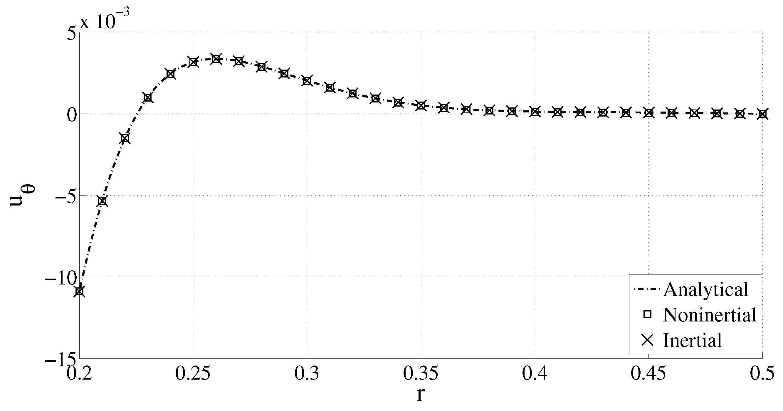
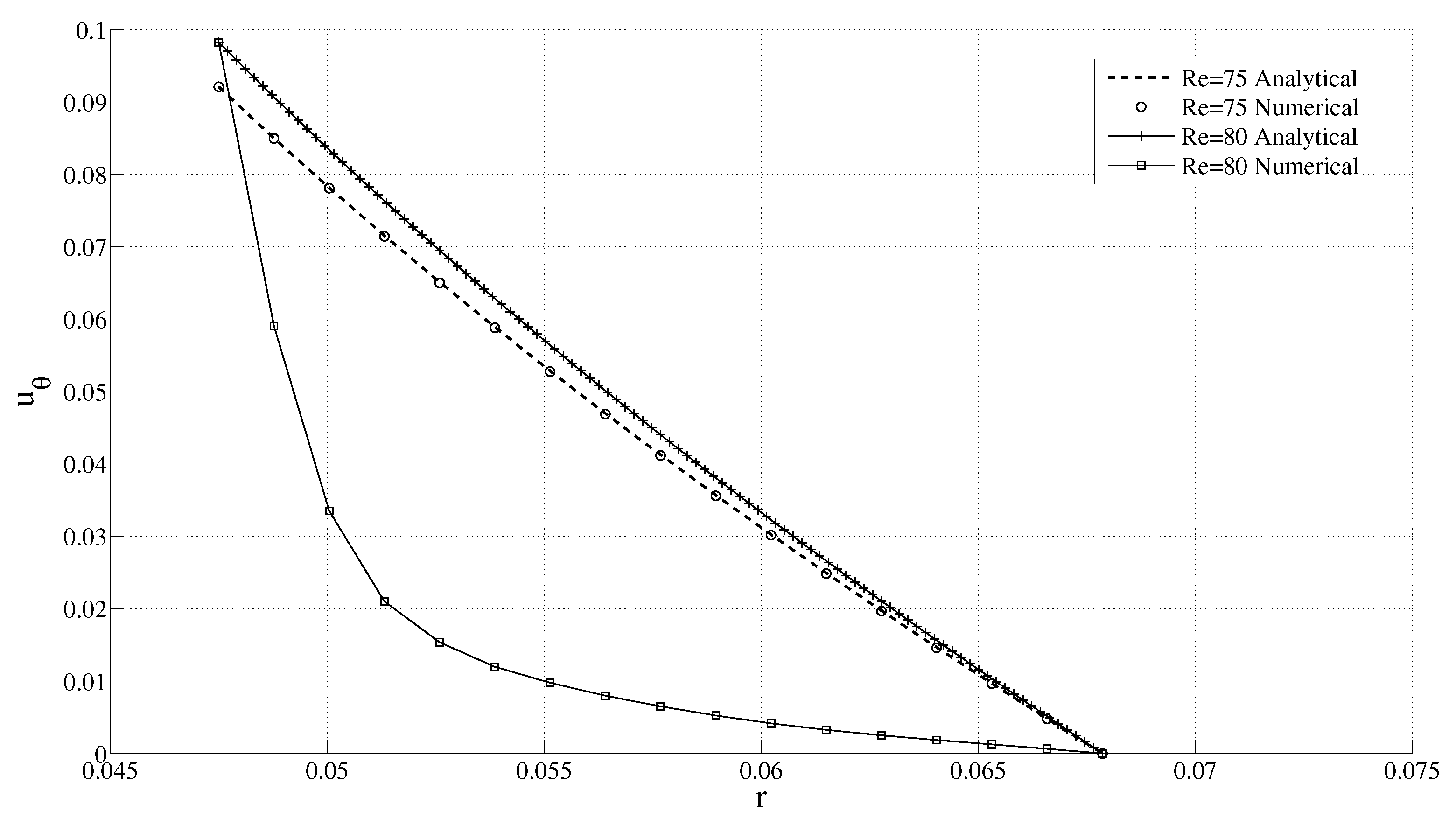
We use 27-node brick elements for meshing the domain in all of the following examples. In all examples, mesh and time step refinement were carried out to ensure convergence of the results with respect to mesh and time step refinement. The noninertial frame solution strategy presented in the previous section is first validated by comparing it against the analytical laminar flow solution presented in [16] for the case where the inner cylinder rotates with a sinusoidally varying speed. Since the analytical solution is presented in an inertial frame of reference, the numerical solution in the noninertial frame of reference is transformed to an inertial frame of reference using Equation (13a) before carrying out the comparison. A numerical solution is also directly found in the inertial frame by imposing a variable velocity on the inner cylinder. We assume the angular speed of the inner cylinder to be $\omega \left(t\right)={\omega }_{0}sin\left(ft\right)$ and that the outer cylinder is fixed. The top and bottom surfaces of the cylinder are traction free. The radii of the inner and outer cylinders are 0.2 and 0.5, respectively. The fluid properties used are $\mu ={10}^{-3}$ and $\rho =1$. The mesh used for finding the solution is $n_r\times n_{\theta }\times n_z=15\times 18\times 1$, and values of the various parameters used are $\alpha =1/2$, $f=1.0$, ${\omega }_0=0.1$, and $t=10$. An almost exact match is found between the numerical and analytical solutions as shown in Figure 1.

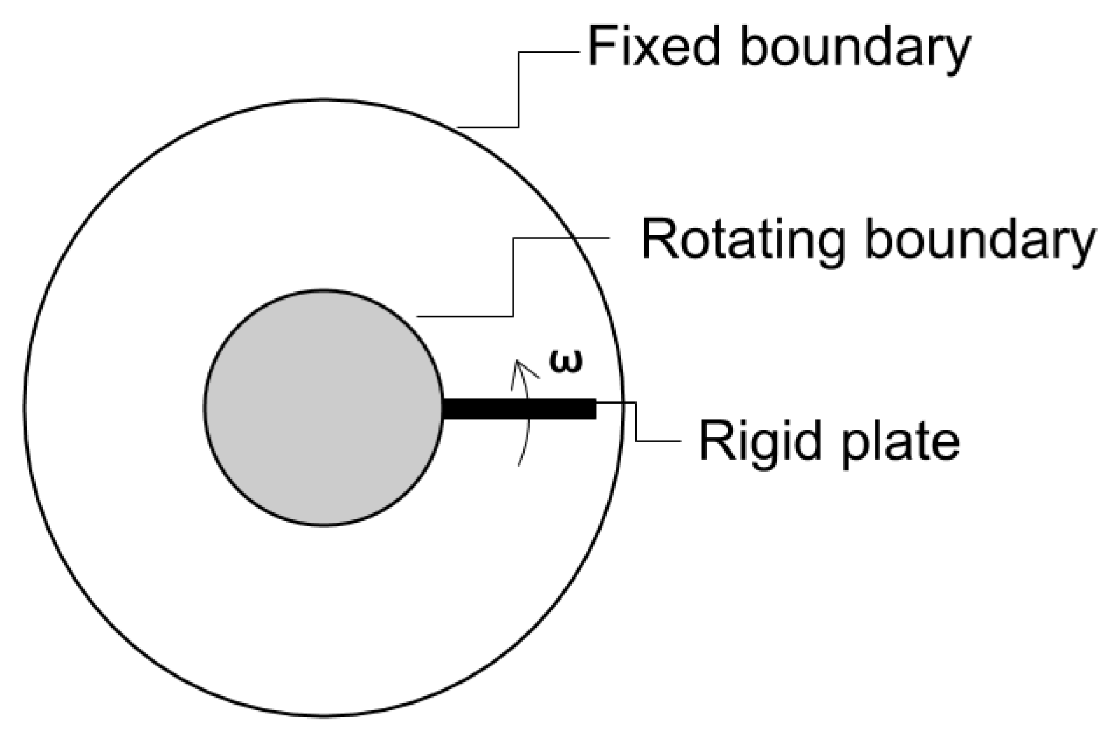
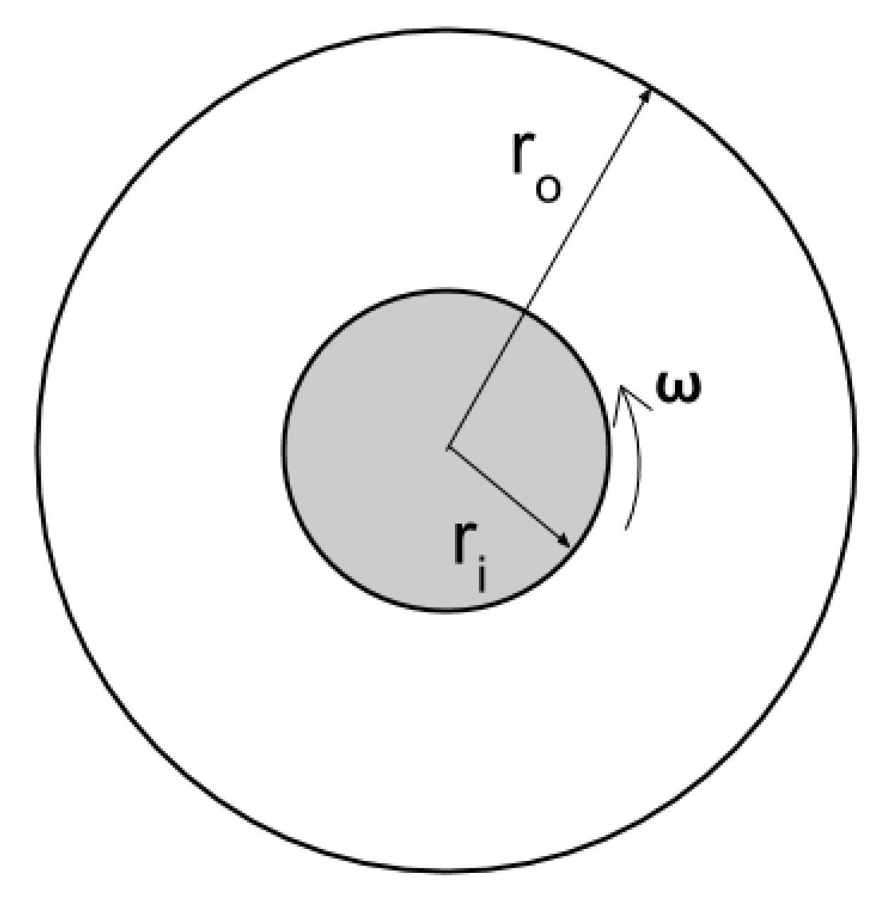
Having validated the noninertial frame formulation, we now present solutions for a problem where no analytical or numerical solutions are available. The problem is to find the flow in the annulus between two concentric cylinders with a rigid plate attached to the inner rotating cylinder (see Figure 2). The angular speed of rotation of the inner cylinder is again assumed to be $\omega \left(t\right)={\omega }_{0}sin\left(ft\right)$. We study the effect of various parameters controlling the flow characteristics—namely, the ratio of plate length along the radial direction to the radial gap between the cylinders, the frequency of oscillation of the inner cylinder, etc. We assume the inner and outer radii, $r_i$ and $r_0$, to be 0.2 and 0.5, respectively. The shape of plate used is wedge-like with central angle 5${}^{\circ }$ . A $15\times 36\times 1$ mesh is used to model the domain. The properties used are $\mu ={10}^{-3}$ and $\rho =1$.

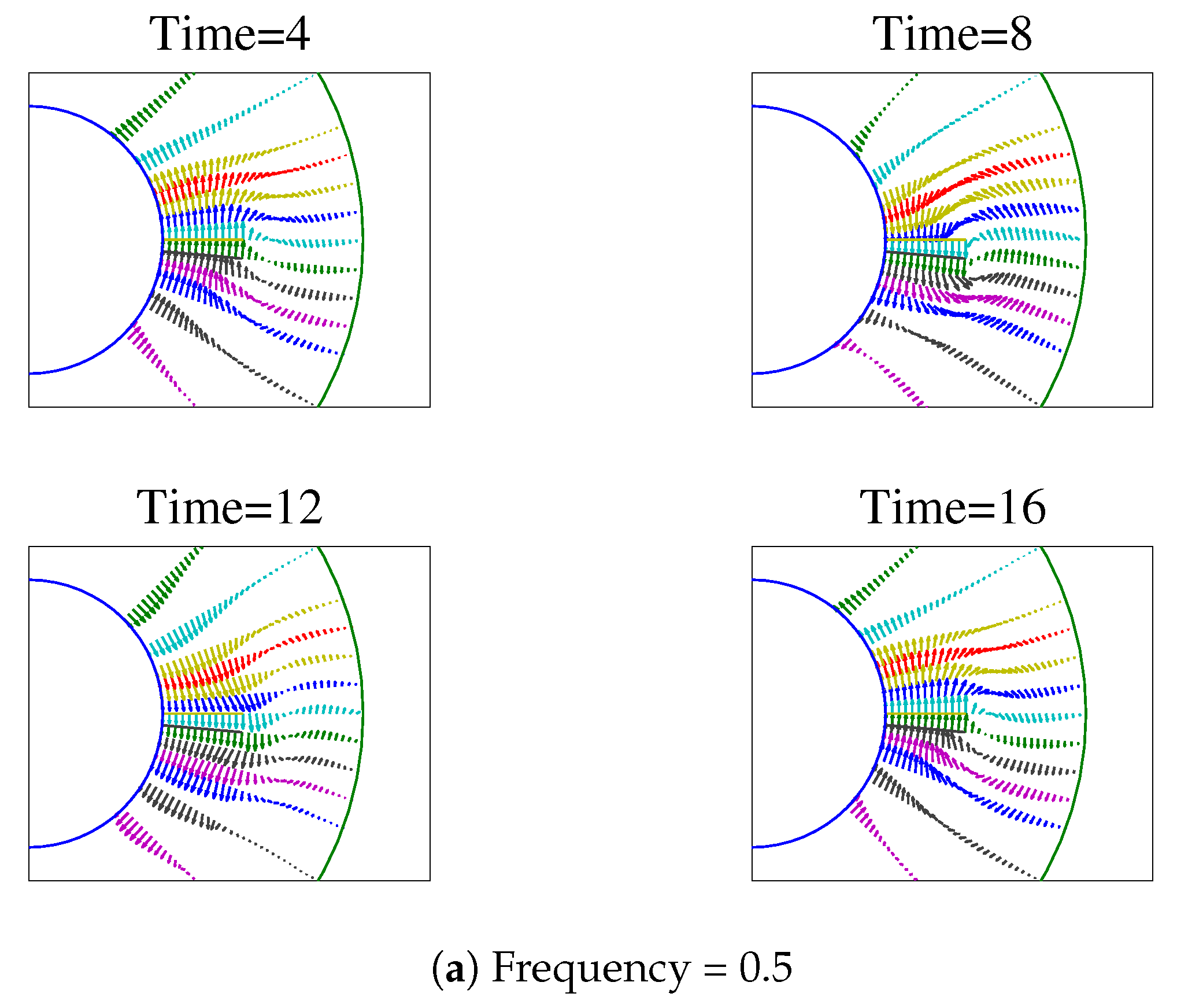
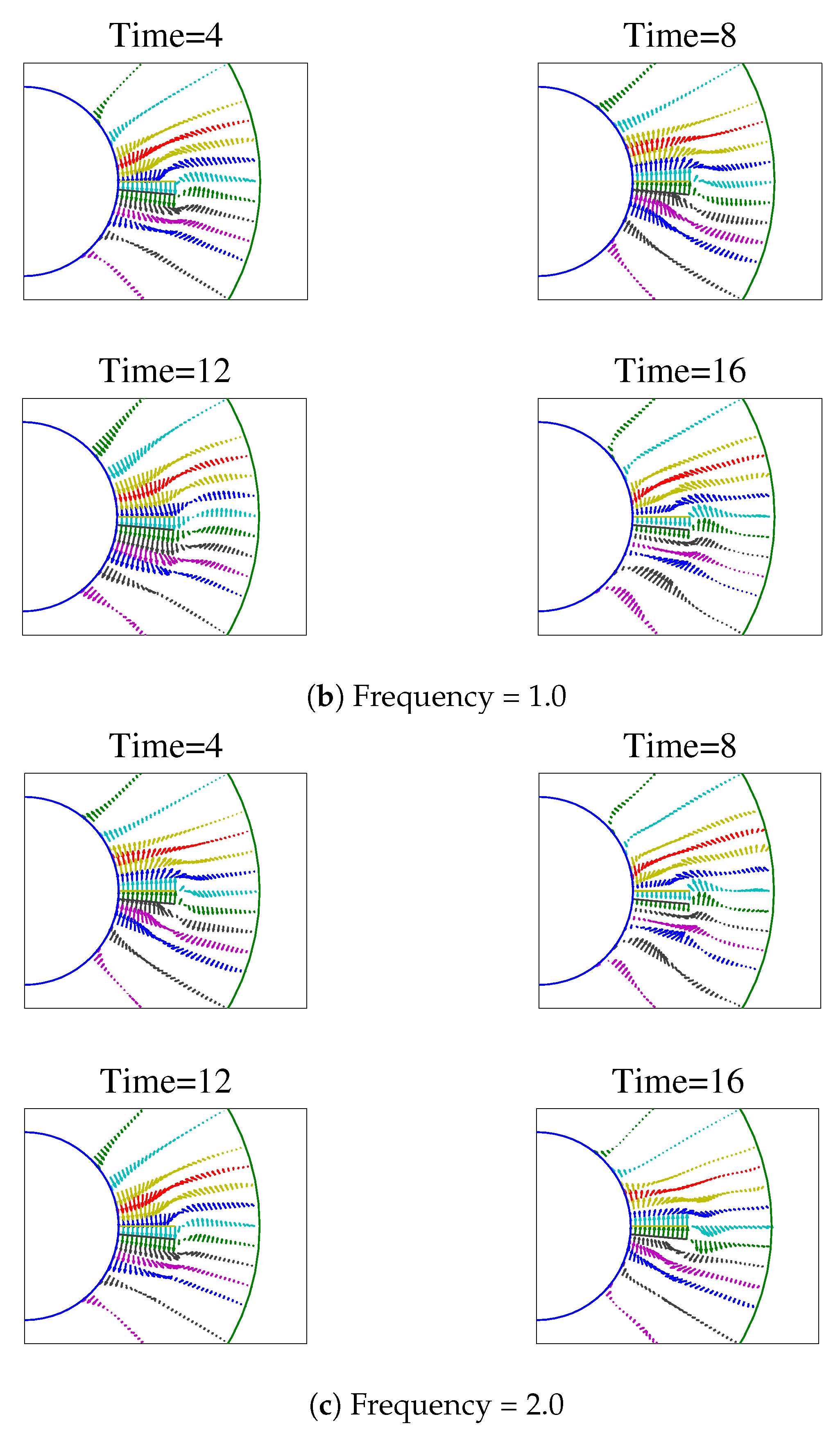
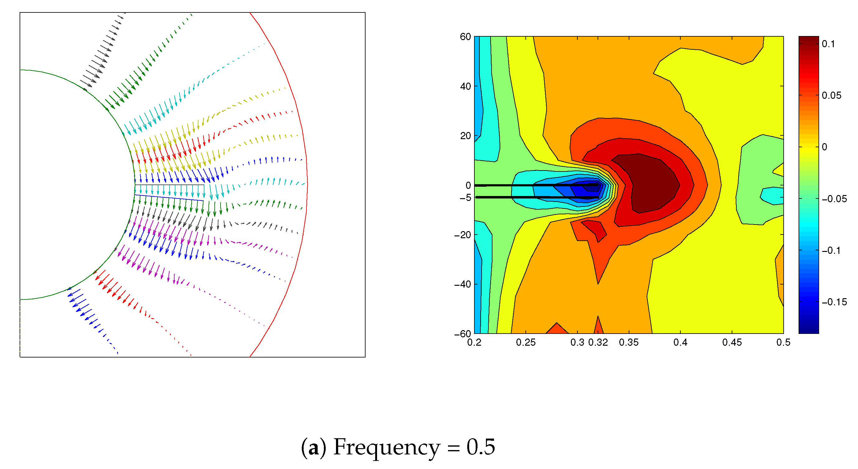
In the subsequent discussion, the velocity flow field is plotted in the mid-plane perpendicular to the axis of the cylinder. It will be seen that vortices form near to the tip of the plate, while the velocity field is almost uniform sufficiently far away from the plate.

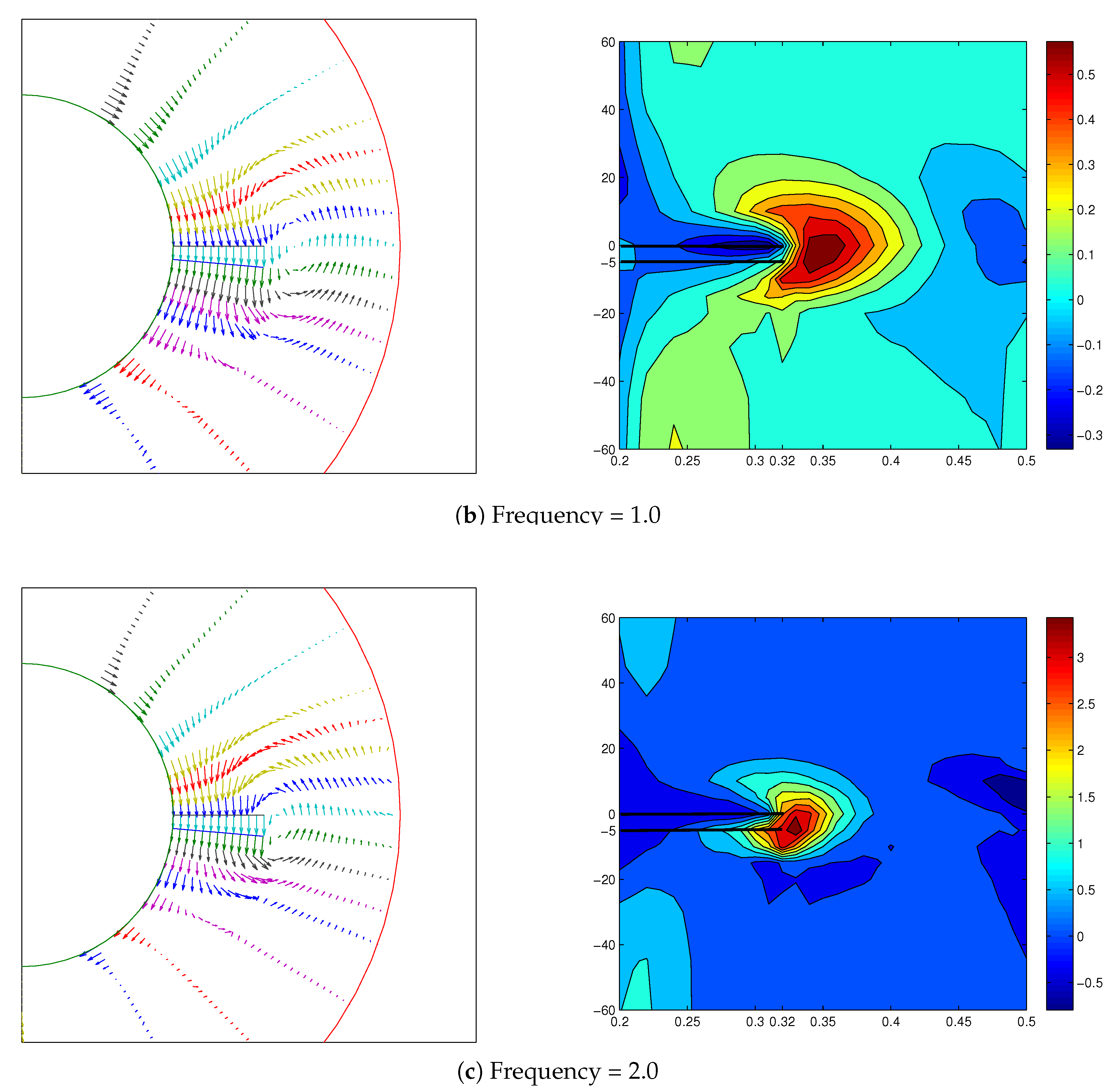
The velocity fields for a width/gap ratio of $0.4$ between the plate and outer cylinder are obtained for $(f,{\omega }_0)=(0.5,0.05)$, $(1,0.1)$, and $(2,0.2)$. Figure 3 shows the velocity fields for the different cases at different times. Similarly, a typical vortex formation at different frequencies at a fixed instant of time is shown in Figure 4. It is seen that a vortex forms on the trailing side of the plate, and is clockwise if the plate is moving anti-clockwise at that instant, and vice versa.

4. Instability in Couette Flow

Most of the literature on instabilities in the case of circular Couette flow (see Figure 5) has focused on the case where the inner cylinder rotates with a constant angular speed. We now present a numerical study to find the critical values of the parameters for the onset of instabilities in case the inner cylinder has a sinusoidally varying speed. It is hoped that these results will prove useful for validating an analytical instability analysis which so far seems to have been confined to the case of constant angular speed.

Taylor [12] was probably the first to conduct such a stability analysis. He found the critical Reynolds number at which the flow becomes unstable for different radii ratios, both analytically and experimentally. At low Reynolds number the flow is azimuthal. As we keep increasing the angular speed of the inner cylinder, at a certain critical Reynolds number ${\mathrm{Re}}_{\mathrm{cr}}$ the flow becomes unstable, and the radial and axial velocity components become nonzero. Taylor studied the effect of the radii ratio on this critical Reynolds number.

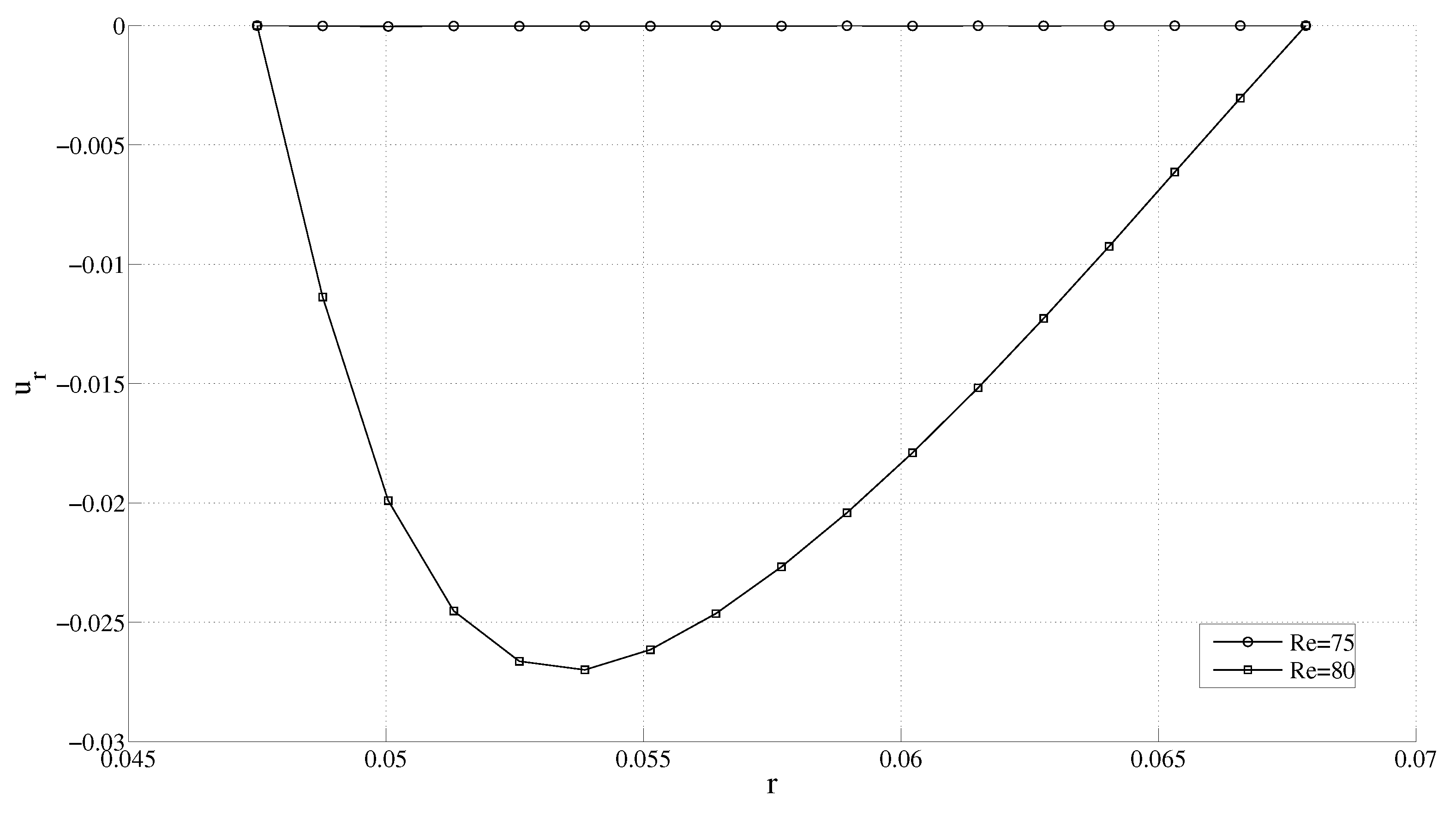
4.1. Constant Angular Speed

Before presenting our results for the varying angular speed case, we first numerically verify that the flow does indeed become unstable at the predicted ${\mathrm{Re}}_{\mathrm{cr}}$ (see

Table 1. Critical Reynolds number for the onset of instabilities for the case of constant angular speed.

Radii Ratio $\mathit{\eta }$	Taylor [12]	Present Work
0.4	–	63
0.5	68.2	–
0.6	71.2	72
0.7	79.5	78
0.8	94.7	89
0.9	131.6	110
0.95	190	175

). Such a numerical verification is important since Taylor’s work is based on linearized stability analysis, which ignores both the nonlinear and transient terms. Since the radial velocity component starts growing (from zero) with the onset of the instability, one can find ${\mathrm{Re}}_{\mathrm{cr}}$ by monitoring this radial and azimuthal velocity component as shown in Figure 6 and Figure 7.

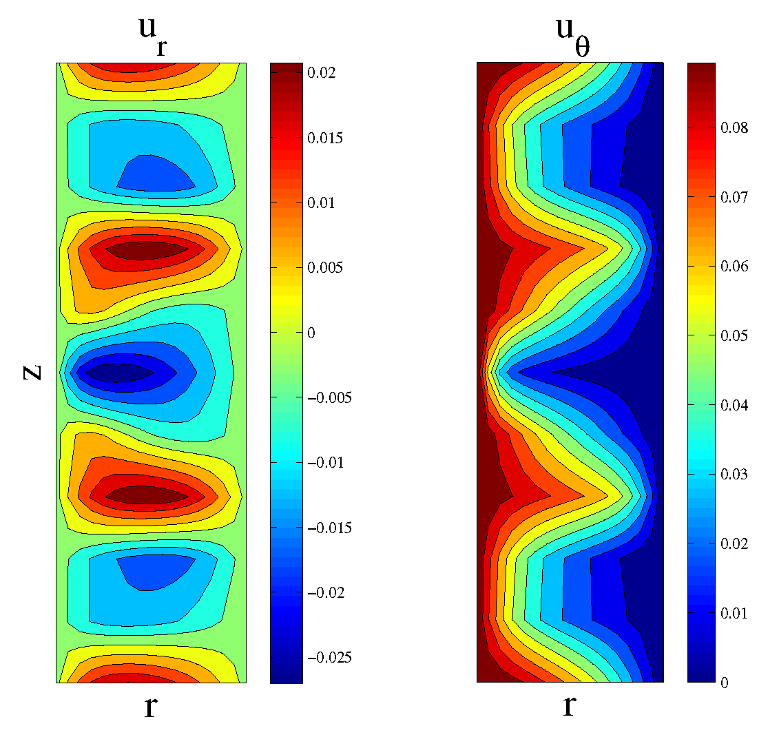
The contour plots for the radial and azimuthal velocity components are similar to those presented in [13], and are shown in Figure 8.

4.2. Sinusoidally Varying Angular Speed

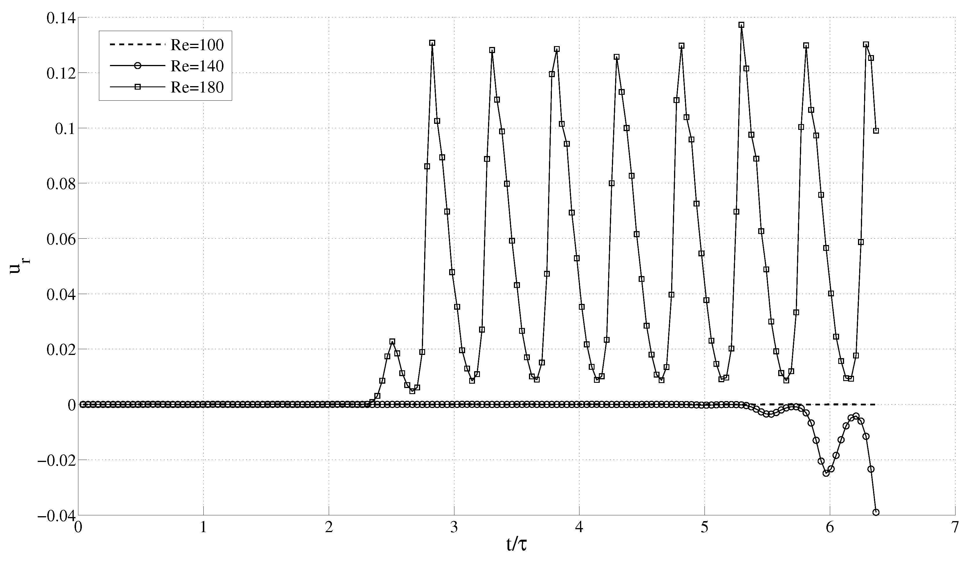
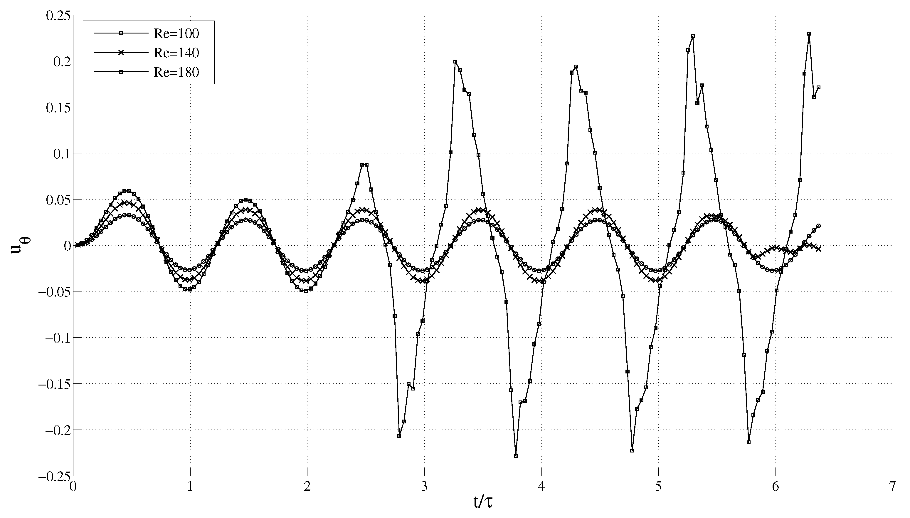
We now find the critical Reynolds number ${\mathrm{Re}}_{\mathrm{cr}}$ for the case where the angular speed of rotation varies with time as $\omega \left(t\right)={\omega }_{0}sin\left(ft\right)$. The radius of the inner cylinder used is $r_i=0.0475$ and the length of the cylinder is chosen to be five times the radial gap. The radius of the outer cylinder $r_o$ is varied to study the dependence of the gap on the flow. The fluid properties used are $\mu =2.5\times {10}^{-3}$ and $\rho =100$. An 8 × 8 × 5 mesh is used to model the domain. For variable angular speed, the Reynolds number is defined based on the amplitude ${\omega }_0$ as $Re=\rho r_i{\omega }_0(r_o-r_i)/\mu$. The effect of various parameters, such as radii ratio $\eta$ and a nondimensional number based on the frequency f, on the critical Reynolds number are studied.

As mentioned, if there is no instability in the fluid flow, it will remain azimuthal with zero radial velocity. However, beyond a certain critical Reynolds number, we clearly observe a non-zero radial velocity component, which is an indication of a centrifugal instability in the fluid. In Figure 9 and Figure 10, the radial and azimuthal velocities at $r=(r_i+r_o)/2$ for varying angular speed are plotted against the number of oscillations. It is seen that for $\mathrm{Re}=100$, the radial velocity $u_r$ is zero, while the azimuthal velocity $u_{\theta }$ follows a sinusoidal pattern. Around $\mathrm{Re}=140$, the $u_r$ component starts growing, and $u_{\theta }$ starts deviating after five cycles, while at $\mathrm{Re}=180$, this deviation occurs after two cycles. This implies that an instability is induced in the fluid at around $\mathrm{Re}=140$. At larger Re, the instability occurs even earlier. In a similar manner, ${\mathrm{Re}}_{\mathrm{cr}}$ can be obtained for different frequencies keeping the geometry fixed, and for different radii ratio keeping the frequency constant.

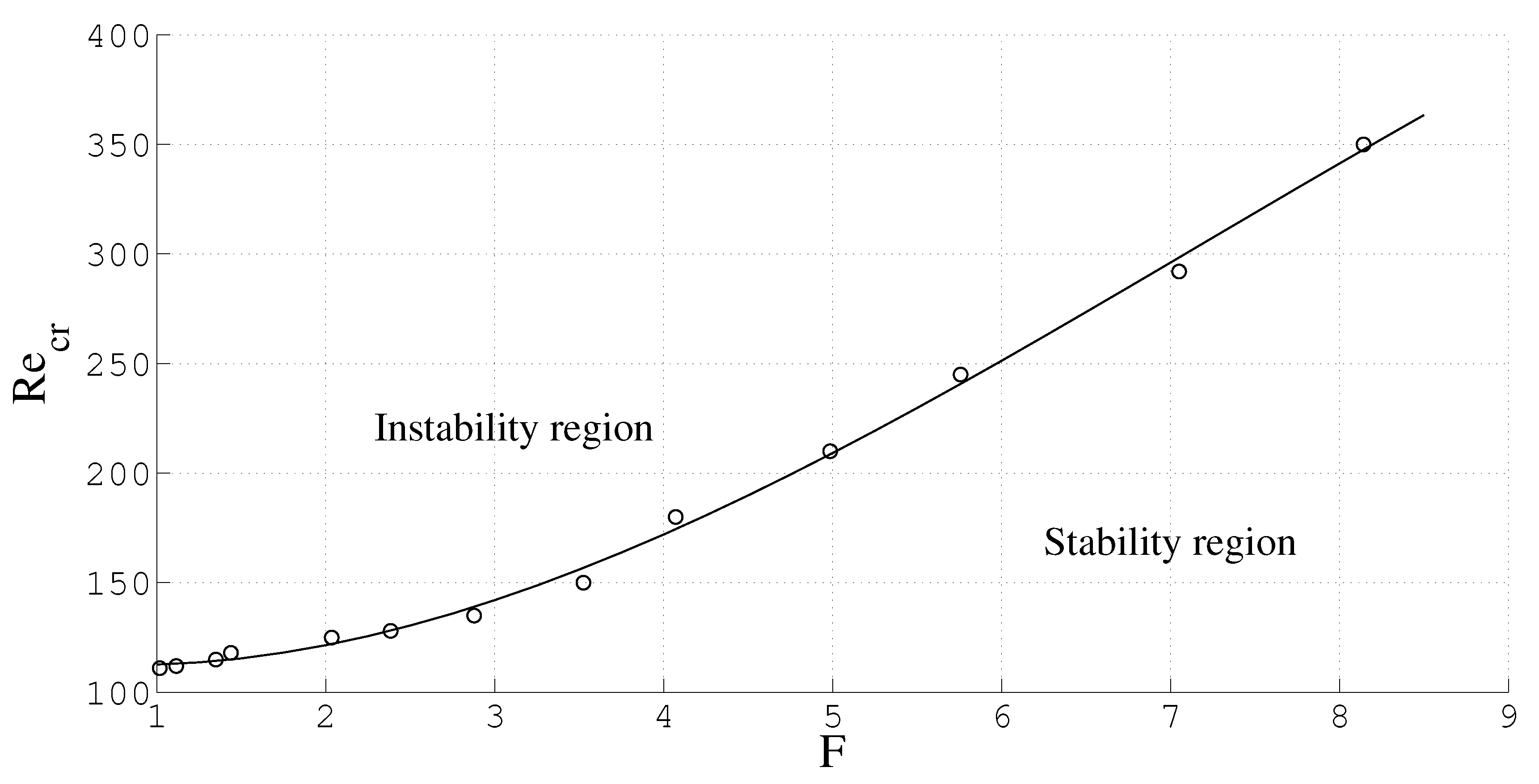
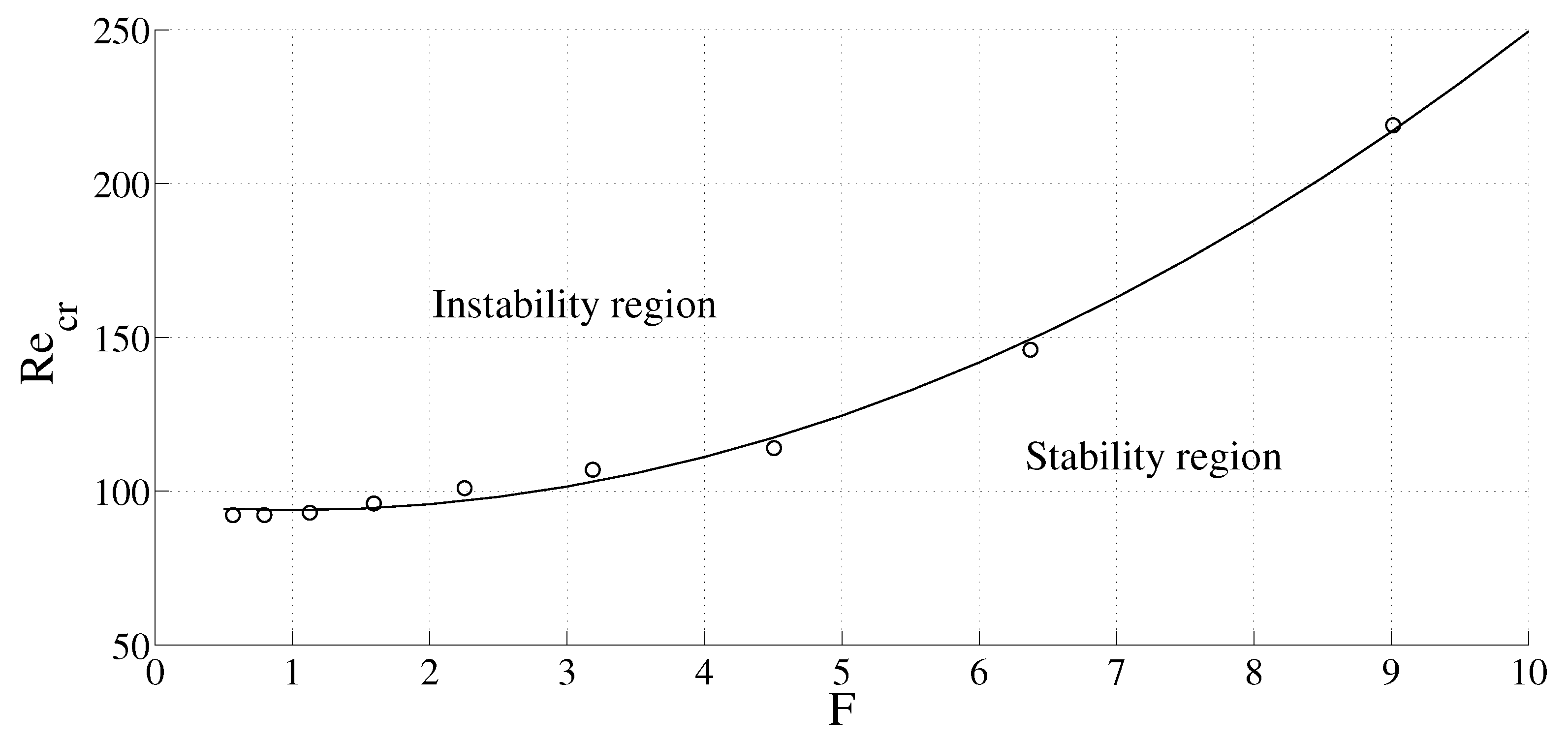
For a geometry with radii ratio $\eta =0.7$ (narrow gap) and $\eta =0.4$ (wide gap), we have studied the dependence of the critical Reynolds number (${\mathrm{Re}}_{\mathrm{cr}}$) on the dimensionless frequency parameter, $F={(d^{2}f/2\nu )}^{1/2}$, where $d=r_o-r_i$, and $\nu$ represents the kinematic viscosity. The frequency f was varied from 0.125 to 8.0. The results are shown in Figure 11 and Figure 12.

It is found that for a particular geometry, ${\mathrm{Re}}_{\mathrm{cr}}$ increases with frequency. When the frequency is higher, the inner cylinder rotates faster so that the fluid layer near the rotating cylinder is exposed to higher Re for small amounts of time due to the higher frequency. The thickness of the fluid layer that gets affected is smaller for higher frequencies, and a higher Re is required to make the flow unstable. Thus, for a fixed geometry, ${\mathrm{Re}}_{\mathrm{cr}}$ increases with frequency.

5. Conclusions and Future Work

In this work, we have developed a finite element strategy for analyzing flows in a noninertial frame of reference which can be used to solve for the fluid flow induced by rotating components inside a circular outer boundary, as is the case in most turbomachinery applications. For this special class of problems, the computational cost is almost the same as that for an inertial frame fixed mesh formulation, and hence much lower compared to an ALE method, where remeshing is typically required.

We have also studied the instabilities that arise in circular Couette flow when the inner boundary rotates with a sinusoidally varying speed. Most of the work in the literature focuses on the case of constant angular speed. The effect of various parameters such as radii ratio and frequency of oscillations on the critical Reynolds number is studied. These results could prove useful for validating a theoretical stability analysis for varying angular speed, which does not seem to have been attempted in the literature, and would obviously be of interest.

References

1. Kim, S.W. A fine grid finite element computation of two-dimensional high Reynolds number flows. Comput. Fluids 1988, 16, 429–444. [Google Scholar] [CrossRef]
2. Kim, S.W.; Decker, R.A. Velocity-pressure integrated versus penalty finite element methods for high-Reynolds-number flows. Int. J. Numer. Methods Fluids 1989, 9, 43–57. [Google Scholar] [CrossRef]
3. Jog, C.S.; Kumar, R. Shortcomings of discontinuous-pressure finite element methods on a class of transient problems. Int. J. Numer. Methods Fluids 2009, 62, 313–326. [Google Scholar] [CrossRef]
4. Takashi, N.; Hughes, T.J.R. An arbitrary Lagrangian-Eulerian finite element methods for interaction of fluid and a rigid body. Comput. Methods Appl. Mech. Eng. 1992, 95, 115–138. [Google Scholar] [CrossRef]
5. Tezduyar, T.E.; Behr, M.; Liou, J. A new strategy for finite element computations involving moving boundaries and interfaces—The deforming-spatial-domain/space-time procedure: I. The concept and the preliminary numerical tests. Comput. Methods Appl. Mech. Eng. 1992, 94, 339–351. [Google Scholar] [CrossRef]
6. Johnson, A.A.; Tezduyar, T.E. Mesh update strategies in parallel finite element computations of flow problems with moving boundaries and interfaces. Comput. Methods Appl. Mech. Eng. 1994, 119, 73–94. [Google Scholar] [CrossRef]
7. Young, Y.L. Fluid-structure interaction analysis of flexible composite marine propellers. J. Fluids Struct. 2008, 24, 799–818. [Google Scholar] [CrossRef]
8. Young, Y.L. Time-dependent hydroelastic analysis of cavitating propulsors. J. Fluids Struct. 2007, 23, 269–295. [Google Scholar] [CrossRef]
9. Young, Y.L.; Baker, J.W.; Motley, M.R. Reliability-based design and optimization of adaptive marine structures. Compos. Struct. 2010, 92, 244–253. [Google Scholar] [CrossRef]
10. Bazilevs, Y.; Hughes, T.J.R. NURBS—Based isogeometric for the computation of flows about rotating components. Comput. Mech. 2008, 43, 143–150. [Google Scholar] [CrossRef]
11. Derksen, J.; Van den Akker, H.E.A. Large eddy simulations on the flow driven by a Rushton turbine. Fluid Mech. Transp. Phenom. 1999, 45, 209–221. [Google Scholar] [CrossRef]
12. Taylor, G.I. Stability of a viscous liquid contained between two rotating cylinders. Philos. Trans. R. Soc. Lond. 1923, 223, 289–343. [Google Scholar] [CrossRef]
13. Meyer-Spasche, R.; Keller, H.B. Computations of the axisymmetric flow between rotating cylinders. J. Comput. Phys. 1980, 35, 100–109. [Google Scholar] [CrossRef]
14. Moser, R.D.; Moin, P.; Leonard, A. A spectral numerical method for the Navier—Stokes equations with applications to Taylor—Couette flow. J. Comput. Phys. 1983, 52, 520–544. [Google Scholar] [CrossRef]
15. Jog, C.S. Continuum Mechanics: Foundations and Applications of Mechanics, Volume I, 3rd ed.; Cambridge University Press: Cambridge, UK, 2015. [Google Scholar]
16. Jog, C.S. Fluid Mechanics: Foundations and Applications of Mechanics, Volume II, 3rd ed.; Cambridge University Press: Cambridge, UK, 2015. [Google Scholar]
Figure 1. Comparison of the analytical and numerical solutions in the inertial and noninertial frames of reference.
Fluids 02 00053 g001
Figure 2. Flow due to oscillation of inner cylinder with a rigid plate attached to it.
Fluids 02 00053 g002
Figure 3. Velocity field in the vicinity of the plate at various times for width/gap = 0.4. (a) Frequency = 0.5; (b) Frequency = 1.0; (c) Frequency = 2.0.
Fluids 02 00053 g003aFluids 02 00053 g003b
Figure 4. Velocity field and vorticity contours in the vicinity of the plate for various frequencies at t = 12 . (a) Frequency = 0.5; (b) Frequency = 1.0; (c) Frequency = 2.0.
Fluids 02 00053 g004aFluids 02 00053 g004b
Figure 5. Circular Couette flow.
Fluids 02 00053 g005
Figure 6. Variation of the radial velocity with radius for different Re for the constant angular speed case.
Fluids 02 00053 g006
Figure 7. Variation of the azimuthal velocity with radius for different Re for the constant angular speed case.
Fluids 02 00053 g007
Figure 8. Contours of the radial and azimuthal velocity components for the constant angular speed case.
Fluids 02 00053 g008
Figure 9. Variation of radial velocity with time for different Re for the varying angular speed case.
Fluids 02 00053 g009
Figure 10. Variation of azimuthal velocity with time for different Re for the varying angular speed case.
Fluids 02 00053 g010
Figure 11. Variation of critical Reynolds number with F for η = 0 . 7 for the varying angular speed case.
Fluids 02 00053 g011
Figure 12. Variation of critical Reynolds number with F for η = 0 . 4 for the varying angular speed case.
Fluids 02 00053 g012