Article

The Use of Semigeostrophic Theory to Diagnose the Behaviour of an Atmospheric GCM

Met Office, Fitzroy Road, Exeter EX1 3PB, UK
Fluids 2018, 3(4), 72; https://doi.org/10.3390/fluids3040072
Submission received: 20 July 2018 / Revised: 25 September 2018 / Accepted: 28 September 2018 / Published: 10 October 2018
(This article belongs to the Collection Geophysical Fluid Dynamics)

Abstract

:
A diagnostic method is presented for analysing the large-scale behaviour of the Met Office Unified Model, which is a comprehensive atmospheric model used for weather and climate prediction. Outside the boundary layer, on scales larger than the radius of deformation, semi-geostrophic theory will give an accurate approximation to the model evolution. In particular, the ageostrophic circulation required to maintain geostrophic and hydrostatic balance against prescribed forcing and a rate of change of the geostrophic pressure can be calculated. In the tropics, the balance condition degenerates to the weak temperature gradient approximation. Within the boundary layer, the semi-geotriptic approximation has to be used because friction and rotation are equally important. Assuming the calculated pressure tendency and ageotriptic circulation match the observed model behaviour, the influence of the large-scale state and the nature of the forcing on the model response can be deduced in a straightforward way. The capabilities of the diagnostic are illustrated by comparing predictions of the ageotriptic circulation from the theory and the model. It is then used to show that the effects of latent heat release can be included by modifying the static stability, and to show the effect of an idealised tropical heat source on the subtropical jet. Finally, the response of the ageotriptic flow to boundary layer heating in the tropics is demonstrated. These illustrations show that the model behaviour on large scales conforms with theoretical expectations, so that the results of the diagnostic can be used to aid the development of further improvements to the model, in particular investigating systematic errors and understanding the large-scale atmospheric response to forcing.

1. Introduction

In common with most other operational weather services and climate research centres, the Met Office uses a comprehensive atmospheric modelling system which is coupled to models of other parts of the Earth system, called the Unified Model (UM) [1]. In common with other centres, the Office undertakes a research programme aimed at improving the performance of the system. A particular focus is the study of systematic errors, where the Office uses a “seamless” approach which exploits the fact that many such errors are present at different model resolutions and time periods [2]. Typically, the errors have large spatial scales. However, correcting them is not straightforward because of the strong coupling between atmospheric variables on large scales resulting from the requirements of geostrophic and hydrostatic balance. Near the equator, the geostrophic requirement degenerates to the “weak temperature gradient” approximation (WTG) [3]. In the boundary layer, friction is also important, leading to “geotriptic” balance [4], where the horizontal pressure gradient is balanced by friction as well as the Coriolis term. This is particularly important in the tropics because it can support horizontal pressure and temperature gradients. The ageotriptic flow is strongly constrained by the need to maintain geotriptic and hydrostatic balance when the model is integrated in time. his constraint would be strictly enforced if the semi-geotriptic (SGT) equations were solved instead of the full governing equations. These generalise the semi-geostrophic (SG) equations by including friction in the lowest order balance. The result is that model changes which appear to be well-suited to reducing systematic errors may not have the intended effect.
In this paper, a diagnostic technique is proposed and illustrated which allows the geotriptic evolution and the ageotriptic circulation of the UM to be calculated for given data. The use of a decomposition of the UM fields into geotriptic and ageotriptic parts is only justified on scales larger than the deformation radius, where the potential vorticity can be well approximated by a function of pressure. In this case, the pressure can be used as the controlling scalar variable and geotriptic winds and hydrostatic temperatures calculated from it. In three-dimensional flow, the requirement that the horizontal scale is greater than the deformation radius becomes a requirement that the aspect ratio is less than the ratio of the Coriolis and Brunt–Väisälä frequencies. The Lagrangian Rossby number also has to be small, restricting the curvature of trajectories. This latter condition is satisfied by fronts and jet streams which are characterised by nearly straight trajectories. However, such flows are only stable to three-dimensional perturbations if the aspect ratio condition is satisfied (see [5], p. 214 and [6]). While these conditions appear very restrictive, they are also the conditions under which coherent anomalies are maintained. Near the equator, the decomposition is only justified outside the boundary layer for flows that are almost zonally symmetric and the WTG holds. These issues are discussed fully in [5]. Within the boundary layer, the usefulness of this method is greatly enhanced because horizontal pressure and temperature gradients can be supported. For instance, it was shown in [7] that using a SGT rather than a SG model allowed large-scale idealised cross-equatorial flows to be simulated.
The diagnostic works by solving the SGT system for a single timestep using UM pressure data and forcing fields from the physical parameterisations. Assuming that the UM solutions can indeed be well approximated by computed SGT solutions on large scales, systematic errors in the UM should be visible in the resulting large scale pressure tendencies and ageotriptic winds. Since the SGT evolution over a timestep is linear in the forcing fields, and is representative of the longer time evolution, it should be possible to relate the systematic errors to particular features of the forcing. More generally, the diagnostic can be used to study the large-scale response of the atmosphere to forcing by calculating the effect of changes to the forcing fields used or to changes in the basic state pressure field. This will aid the study of issues such as tropical–extratropical interaction, and its dependence on the large-scale flow.
The semi-geostrophic (SG) model was originally introduced by Eliassen [8] as an alternative description of large-scale flows to the quasi-geostrophic model of Ref. [9]. It is based on what was subsequently called the Type II geostrophic scaling by Phillips [10] and in particular allows full variation of the static stability and Coriolis parameter. It is reviewed with a broader perspective by Eliassen [11]. The model was then reintroduced by Hoskins [12] to study frontogenesis. In that study, a constant Coriolis parameter is used, which allows the equations to be transformed to a simpler form by using the geostrophic coordinate transformation. This version of the SG model can be solved for large times in isentropic coordinates by using optimal transport methods, as reviewed by Cullen [5]. Once the variable Coriolis parameter is included, the equations have to be solved in physical space. Formal arguments demonstrating how the equations can then be solved were given by Cullen et al. [13,14]. However, the only rigorous result so far is limited to short times, as given by Cheng et al. [15]. This result is sufficient to justify the diagnostic procedure used in this paper, where the equations are solved for a pressure tendency and ageostrophic wind at a single time in the manner of Ref. [16]. The extension to the semi-geotriptic (SGT) model was described by Beare et al. [4]. This is very important because it allows a realistic lower boundary condition. The need to use a nonlinear formulation of vertical momentum diffusion has meant that no rigorous treatment of this set of equations is yet available.
In the UM, the large-scale fields will be close to geotriptic and hydrostatic, so the ageotriptic circulation required to maintain this balance against forcing will be predicted by SGT theory. Thus, if the UM forcing is diagnosed and input into the calculation of a single SGT timestep, the resulting ageotriptic flow should form a part of the ageotriptic flow actually produced by the UM. The total UM circulation will also contain transients, not subject to this constraint. In studying systematic UM errors, it is useful to determine what aspects of the circulation are constrained by the balance requirement, and which parts are evolving independently.
This calculation is a three-dimensional generalisation of the widely used Sawyer–Eliassen equation (SEE) (e.g., [17]). An important feature of SEE is that the calculation of the ageostrophic circulation depends strongly on the static and inertial stability of the large-scale state. The effect of moisture on static stability can be included. Most of the applications of the SEE are in a vertical cross-section, where it is easy to justify its use. Examples specifically exploiting SG theory are found in [18,19]. Three dimensional solutions using SG were given by Wernli et al. [20], where the results are compared with solutions of the full equations using idealised data, and Ragone et al. [21], where the results are compared with other idealised models. Examples including the boundary layer using SGT theory were given by Beare et al. [4]. In three-dimensions, the validity of the SEE requires SG theory to be accurate, which implies the restrictions discussed above. This has limited its use.
In the next section, the analytical formulation of the diagnostic is presented. The method works from the pressure field, which implies geotriptic winds and hydrostatic potential temperatures. As noted above, this is appropriate on scales where the SGT approximation is valid. However, UM data will contain non-geotriptic motions which affect the pressure, so steps have to be taken to minimise their effect on the diagnostic calculation. The equation for the pressure tendency is an elliptic equation, and the solution procedure is described. The discretisation of the equation requires care over orography, and it is essential to follow the principles of the UM scheme.
Since systematic errors in the UM will typically have a large scale signal, it should be possible to reproduce them by applying the diagnostic to a large number of cases and averaging the results. Before doing so, however, it is necessary to demonstrate the usefulness of the diagnostic in individual cases. The results section therefore includes four examples illustrating the performance of the diagnostic. The first is a comparison of the actual ageotriptic circulation produced by the UM in the extratropics with that calculated using SGT theory. This shows that the procedure is viable with full UM data subject to the extra processing noted in the previous paragraph. The second example calculates the vertical motion required to maintain large scale balance in cloudy air assuming moist static stability, and then inferring the latent heat release from the difference between the potential temperature increment calculated using this vertical motion with moist and dry static stability. This should represent the “forced” part of the latent heating actually calculated by the UM physics. The third example shows the effect of an idealised tropical heat source on the extratropical flow following [22]. There is geostrophic adjustment in the north–south direction, as illustrated by Schubert et al. [23], which should be realistic. The diagnostic also adjusts in the east-west direction, but except for very long forcing timescales this would in reality generate a tropical wave, as in the simulations of Jin, et al. [22] using an idealised general circulation model. The final example shows that thermally forced ageotroptic circulations in the boundary layer can be simulated.

2. Materials and Methods

2.1. The SG Approximation to the UM Equations

The diagnostic procedure uses the SGT and hydrostatic approximation in the deep atmosphere compressible equations solved by the UM [24]. No other approximations are made, so that the diagnostic should extract the geotriptic part of the UM evolution.
We first write the equations in Lagrangian form. The equations are written in spherical polar and terrain-following coordinates ( λ , ϕ , η ) , where λ , ϕ are longitude and latitude, and η is the model level number. The true radial coordinate is r. The boundary layer momentum mixing is included, with stability dependent diffusion coefficient K m as calculated by the UM. A derivative with respect to r is interpreted as a derivative with respect to η multipled by η / r with ( λ , ϕ ) constant.
D u D t + c p d θ v π + 2 Ω × u = g + r K m u h r + S u , D θ v d D t = S θ v d , D μ D t = S μ , ρ d t + · ( ρ d u ) = 0 .
where
ρ d = p 0 R d π 1 κ d κ d θ v d , R d = κ d c p d , μ = Σ m X , X = v , c l , c f , θ v = θ v d 1 + μ .
In these equations, u is the vector velocity field and θ v the virtual potential temperature with θ v d the virtual potential temperature for dry air. ρ d is the density of dry air and π the Exner pressure p p 0 κ d . p 0 is a reference pressure, R d is the gas constant for dry air and c p d is the specific heat of dry air at constant pressure. κ d is defined by the second part of Equation (2). m X indicates the mixing ratio of various moisture constituents denoted by X and μ is the sum of all these mixing ratios. Ω is the Earth’s rotation vector and g is the gravitational and centrifugal vector. S x is a source term for variable x. The suffix h denotes horizontal components.
The lower boundary condition is no slip. The upper boundary condition is a rigid lid.
The semi-geotriptic approximation in spherical geometry assumes first that the shallow atmosphere hydrostatic approximation holds [25], so that the rotation term 2 Ω × u is replaced by its horizontal components ( f v , f u ) where f = 2 Ω sin ϕ , ϕ is the latitude, and that the gravitational vector g only has a component in the local vertical. Then, the vertical momentum in Equation (1) becomes
c p d θ v π r = g .
To understand the solutions, we subtract a reference state π 0 ( r ) satisfying
c p d θ 0 π 0 r = g ,
where θ 0 is a constant, from π , giving
c p d θ v π r = g θ θ 0 ,
where θ = θ v θ 0 . The Brunt–Väisälä frequency N is then given by
N 2 = g θ 0 θ r .
Assume typical scalings P and Θ for π and θ , ignore μ and assume typical length scales L and H in the horizontal and vertical. Then, π / r P / H and the horizontal pressure gradient term h ϕ P / L . In some regimes, the ratio of horizontal and vertical gradients of π may be much less than H / L if π is close to hydrostatic balance with a spatially uniform stably stratified reference profile θ ( r ) . This is not generally the case on large scales with real data, particularly because of large horizontal variations of the tropopause height.
The geostrophic regime is characterised by the terms c p d θ v h π in the horizontal momentum equations having the same magnitude as ( f v , f u ) . Equations (5) and (6) show that c p d θ v π / r N 2 H . Defining U as a horizontal velocity scale, the geostrophic regime requires that f U N 2 H 2 / L . Now, define the dimensionless Rossby and Froude numbers, R o and F r , respectively, by
R o = U f L , F r = U N H .
Then, geostrophic balance requires R o = F r 2 . The semi-geostrophic regime is thus characterised by a small parameter ϵ = R o = F r 2 . The radius of deformation L D is defined as N H / f , so that L / L D = O ( ϵ 1 2 ) .
Geotriptic balance requires that the horizontal pressure gradient is comparable to the friction term. If K is a typical magnitude of the momentum diffusion coefficient K m , this requires that N 2 H 2 / L K U / h 2 where h H is a typical boundary layer depth. This scaling is discussed in [26].
Since the aim is to apply the diagnostic procedure directly to model data, the subtraction of a basic state as in Equation (4) is not used. Therefore, we define geotriptic and hydrostatic balance and the geotriptic wind u e = ( u e , v e ) consistently with Equation (1) by
c p d θ v h π ( f v e , f u e ) = r K m u e r , c p d θ v π r = g .
Then, the first part of Equation (1) can be approximated to O( ϵ 2 ) outside the boundary layer by
D u e D t f ( v v e , u e u ) = r K m ( u e u h ) r + S u , c p d θ v π r = g .
Note that the full velocity u is used in the Lagrangian time derivative D / D t as in the geostrophic momentum approximation. Equation (9) is only accurate to O( ϵ ) in the boundary layer, assuming h / H is independent of ϵ . As discussed in [26], it is more typical for h / H to decrease with ϵ ; that paper suggests h / H ϵ 0 . 7 . The SGT approximation to Equation (1) consists of Equations (8), (9) and Equation (1) after the first. The boundary conditions are the same as for Equation (1).

2.2. The Diagnostic Equations

The diagnostic equations are based on the original Equation (1). The equations are written in Eulerian form as in [16] to derive an Eulerian pressure tendency and an equation for the ageotriptic winds. The principle of the derivation is the same as that for the basic two-dimensional SEE (e.g., [27], p. 287). The first part of Equation (8) is written
f v e + r K m u e r = c p d θ v r cos ϕ π λ π r r λ , f u e + r K m v e r = c p d θ v r π ϕ π r r ϕ .
where the horizontal derivatives are computed on η surfaces.
Equation (10) can be used to generate a single equation for u e (eliminating v e terms):
f 2 u e + r K m 2 r 2 K m u e r = r K m r c p d θ v r cos ϕ π λ π r r λ f c p d θ v r π ϕ π r r ϕ .
Given values of π , Equation (11) can be used to calculate u e . The lower boundary condition is that u e = v e = 0 at η = 0 . It is assumed that K m is zero above some η level below the upper boundary, so that setting K m = 0 there will generate an upper boundary condition for Equation (11). For larger values of η , Equation (11) can be solved independently at each level.
The first part of Equation (9) and the second and third parts of Equation (1) can then be rewritten in Eulerian form as
u e t + u · u e f ( v v e ) = r K m ( u e u ) r + S u , v e t + u · v e + f ( u u e ) = r K m ( v e v ) r + S v , θ v t + u · θ v = 1 1 + μ S θ v d θ v d ( 1 + μ ) 2 S μ S θ v .
Equation (12) can be rewritten as
Q u u e v v e w + t v e u e θ v = H ,
where
Q = f + 1 r cos ϕ v e λ + u e tan ϕ r 1 r v e ϕ + r K m r v e r 1 r cos ϕ u e λ + v e tan ϕ r r K m r f 1 r u e ϕ u e r 1 r cos ϕ θ v λ 1 r θ v ϕ θ v r
and
H = u e · v e + S v u e · u e S u u e · θ v + S θ v .
We now derive a single equation for the pressure tendency. Differentiating geotriptic balance (the second part of Equation (10)) with respect to time, and assuming K m is time independent, gives
f u e t + r K m r v e t = c p d θ v r t π ϕ π r r ϕ + 1 r π ϕ π r r ϕ c p d θ v t .
Next, define
B = f r K m r 0 r K m r f 0 0 0 g / θ v .
Then, using Equation (10), the similar equation for π / λ and the relation
c p d θ v t π r = g θ v θ v t ,
obtained by differentiating hydrostatic balance (the second part of Equation (9)) with respect to time, we can write
B v e t u e t θ v t = c p d θ v t 1 r cos ϕ π λ π r r λ 1 r π ϕ π r r ϕ π r + 1 r cos ϕ π λ π r r λ 1 r π ϕ π r r ϕ 0 c p d θ v t .
Using Equation (10), the second term on the right hand side can be replaced by
1 θ v B v e u e 0 θ v t .
Outside the boundary layer, this can be rewritten as
B v e θ v θ v t u e θ v θ v t 0 .
and so this term can be amalgamated with the left hand side giving
B v e t v e θ v θ v t u e t + u e θ v θ v t θ v t or B θ v t v e θ v θ v t u e θ v θ v t .
Within the boundary layer, we note that the vertical variation of u e / θ v will be dominated by the vertical variation of u e , so we use the amalgamated form of the left hand side of Equation (19) in the boundary layer also. This additional approximation is needed to allow the reduction to a single equation to proceed.
Using the third part of Equation (12), we can then rewrite Equations (13)–(15) as
B Q u u e v v e w + c p d θ v t 1 r cos ϕ π λ π r r λ 1 r π ϕ π r r ϕ π r = B H
where
Q = f + θ v r cos ϕ λ v e θ v + u e tan ϕ r θ v r ϕ v e θ v + r K m r θ v r v e θ v θ v r cos ϕ λ u e θ v + v e tan ϕ r r K m r f θ v r ϕ u e θ v θ v r u e θ v 1 r cos ϕ θ v λ 1 r θ v ϕ θ v r
and
H = ( u e θ v ) · v e θ v + S v v e S θ v θ v ( u e θ v ) · u e θ v S u + u e S θ v θ v u e · θ v + S θ v .
We can then write BH as G where
G = f u e θ v r cos ϕ λ v e θ v f u e 2 tan ϕ r f v e θ v r ϕ v e θ v + f S v f v e S θ v θ v r K m r u e S θ v θ v f u e θ v r cos ϕ λ u e θ v f u e v e tan ϕ r + f v e θ v r ϕ u e θ v f S u + f u e S θ v θ v r K m r v e S θ v θ v g u e r θ v cos ϕ θ v λ g v e r θ v θ v ϕ + g S θ v θ v .
Since B and Q involve values at adjacent levels, it is impractical to eliminate u directly from Equation (20) to solve for π t . To solve Equation (20) reasonably accurately, a preconditioning is required. To invert BQ , we therefore approximate BQ by an invertible matrix P , so that Equation (20) is replaced by
P u u e v v e w + c p d θ v t 1 r cos ϕ π λ π r r λ 1 r π ϕ π r r ϕ π r = G ,
where P = P 1 P 2 P 3 . P 1 is given by
P 1 = f 2 + r K m 2 r 2 K m r 0 0 0 f 2 + r K m 2 r 2 K m r 0 0 0 1 .
P 2 is given by
P 2 = f 2 + f θ v r cos ϕ λ v e θ v + f u e tan ϕ r f θ v r ϕ v e θ v f θ v r v e θ v f θ v r cos ϕ λ u e θ v + f v e tan ϕ r f 2 f θ v r ϕ u e θ v f θ v r u e θ v g r cos ϕ θ v θ v λ g r θ v θ v ϕ g θ v θ v r ,
and
P 3 = f 2 0 0 0 f 2 0 0 0 1 .
We next have to eliminate u using the continuity equation and equation of state, which are the fourth and fifth parts of Equation (1). In ( λ , ϕ , η ) coordinates, we have u = ( u , v , η ˙ ) and
η ˙ r η = w u r cos ϕ r λ v r r ϕ .
This can be rewritten as
R u v w = u v η ˙ .
The continuity equation then takes the form
t r 2 ρ d r η + 1 cos ϕ λ r ρ d u r η + ϕ r ρ d v cos ϕ r η + η r 2 ρ d η ˙ r η = 0
Now, applying the operator
· r 2 ρ d r η R
to Equation (24) and using Equation (29) gives
t r 2 ρ d r η + · r 2 ρ d c p d θ v r η RP 1 t r π = · r 2 ρ d r η RP 1 G + 1 cos ϕ λ r ρ d u e r η + ϕ r ρ d v e cos ϕ r η .
Next, differentiating the equation of state with respect to time gives
κ d 1 κ d π 1 κ d π t ρ d θ v d + π κ d 1 κ d ρ d t θ v d + π κ d 1 κ d ρ d θ v d t = 0 .
Removing common factors, and using Equation (18) and the final part of Equation (2) to evaluate the final term of Equation (31) gives
κ d 1 κ d π t ρ d θ v d + π ρ d t θ v d π ρ d c p d θ v 2 g t 1 ( 1 + μ ) π r = 0 .
We now substitute Equation (32) into Equation (30) to give
κ d 1 κ d ρ d π r 2 r η π t + r 2 r η ρ d c p d θ v 2 g θ v d t 1 ( 1 + μ ) π r + · r 2 ρ d c p d θ v r η RP 1 t r π = · r 2 ρ d r η RP 1 G + 1 cos ϕ λ r ρ d u e r η + ϕ r ρ d v e cos ϕ r η .
Apart from the small term t 1 ( 1 + μ ) , which needs to be diagnosed separately, this is an elliptic equation for π / t , which can be solved. Boundary conditions are required at the top and bottom. The boundary conditions inherited from Equation (1) imply that η ˙ = 0 at the top and bottom, which implies a zero gradient of
r 2 ρ d c p d θ v r η RP 1 t r π .
Equation (28) and the no slip lower boundary condition then implies that w = 0 at the lower boundary also. Then, Equations (20) and (22) reduce to
c p d θ v π r = S θ v .
We can then calculate the ageotriptic velocity u u e , v v e and w by applying P 1 to Equation (24).

2.3. Application

The right hand side of Equation (33) shows that the evolution is driven by the divergence of the forcing vector G and the divergence of the geotriptic wind ( u e , v e ) . Changes to the forcing with zero divergence, in the sense of the first term on the right hand side of Equation (33), will not affect the evolution. Such changes will simply alter the ageostrophic wind vector ( u u e , v v e , w ) so that Equation (20) is satisfied. This demonstrates that changes to the forcing in the UM may have a much smaller effect on the large-scale evolution than might be expected.
Using the definition of G in Equation (23), we see that the first term on the right hand side of Equation (33) includes geotriptic advection of the momentum and potential temperature, the dynamical forcing, together with the external forcing terms S which are generated by the UM physics. The second term on the right hand side would be just the divergence of the geostrophic wind if the boundary later were not included. This would be zero in pressure coordinates with a constant Coriolis parameter. There is a contribution from variations in the Coriolis parameter, which gives the effect of Rossby wave propagation on the pressure tendency. Since the divergence calculation used to derive Equation (33) is in terrain-following coordinates, the orography will also contribute to this term through the horizontal variations of r η . This shows how the orography can have a strong effect on the large-scale flow.
Moisture will interact strongly with the diagnostic procedure through the reduction of the effective static stability by latent heat release. This effect has been studied, for instance, by Booth et al. [28]. In the UM, the thermodynamic equation, which is the second part of Equation (1), includes the terms
w θ v d r = S L H ,
where S L H is the part of the forcing term resulting from latent heat release. This term is dominated by the term D q s a t D t , where q s a t is the saturated mixing ratio which is largely a function of temperature. In a simple form, this can be represented by calculating a cloud fraction weighted static stability, where θ v / r is the stability of the unsaturated air allowing for the virtual temperature effect and θ e * / z is the moist stability, where θ e * is the equivalent potential temperature calculated assuming saturation. w is not known in advance, so the idea that latent heating only occurs with upward motion cannot be used as the problem becomes nonlinear in w. The use of cloud fraction weighting avoids this problem, as evaporation will occur if w is negative in cloudy regions. If α is the cloud fraction, we set
θ v r e f f = ( α θ e * + ( 1 α ) θ v ) ) r .
A more sophisticated approach would be to use a formula set out in [29] for wave propagation in inhomogeneous media. Applying this to a wet/dry mixture gives a modified Brunt–Väisälä frequency as
N e f f 2 = α N d 2 + ( 1 α ) N w 2 N w 2 N d 2 1 ,
where
N w 2 = g θ θ e * r , N d 2 = g θ θ v r .
We thus replace θ v r in Q , Equation (21), by
θ v r e f f = α θ v r + ( 1 α ) θ e * r θ e * r θ v r 1 .
The model value of cloud fraction α can be used, provided again that small space and time scales are excluded.
If the temperature increment S L from the large scale precipitation scheme is added to S, the solution of Equation (20) will become
B Q u u e v v e w + c p d θ v t 1 r cos ϕ π λ π r r λ 1 r π ϕ π r r ϕ π r = B H + 0 0 S L .
The solution of Equation (40) for π t is identical to that of Equation (20) if the element θ v r in Q in that equation is replaced by θ v r e f f as in Equation (39) and
S L = w θ v r θ v r e f f .
This will be approximately true if the latent heat release is dominated by the effects of vertical motion. This is illustrated in Section 3.3.

2.4. Computational Aspects

The elliptic equation (33) is solved by a preconditioned generalised conjugate residual method which requires explicit evaluation of the elliptic operator on the left hand side for a given estimate of π / t , and an evaluation of the right hand side. The preconditioning is done by a vertical matrix inversion, which uses a tridiagonal solver, and a horizontal smoother.
Given π , K m from model data, solve Equations (10) and (11) for ( u e , v e ) . Care has to be taken in calculating the right hand side of Equation (10) because the two terms cancel strongly over orography. The scheme, based on that used in the UM and exploiting hydrostatic balance, is
c p d θ v r cos ϕ π λ π r r λ c p d θ ¯ v λ δ λ π + g δ λ r ,
where δ λ indicates a central difference in the λ direction divided by 2 r cos ϕ δ λ . A similar scheme is used in the ϕ direction. Solving Equation (11) then involves inverting a N × N penta-diagonal matrix at each horizontal gridpoint, where N is the number of model levels and K m is nonzero.
Next, use ( u e , v e ) to evaluate the components of P 2 , Equation (26). Central differencing has to be used because the upwind direction is not known in advance. The vertical stability is evaluated more accurately as a vertical second difference of π . The values are filtered towards a zonal mean close to the equator in order to remain within the validity of the theory. If Equation (36) or (39) is used, the relative humidity, moisture content and cloud fraction are used to calculate the effective static stability.
Next, calculate the eigenvalues of P 2 at each point. Modify P 2 as necessary to remove negative eigenvalues. This can be done by first replacing any negative diagonal terms by suitable reference values, such as 10 10 in the first two rows and 10 6 in the third, and then rescaling the off-diagonal terms as required.
Next, construct the vertical pre-conditioner. If P 2 i j is the value of the ( i , j ) component of P 2 , calculate the rms value PI r m s of P 233 1 as a function of model level. Then, at each horizontal gridpoint, we precondition Equation (33) by replacing the left hand side by
A π t C 1 κ d 1 κ d ρ d π r 2 r η π t + · r 2 ρ d c p d θ v r η RPI v t r π .
C 1 is set to 100 in the examples illustrated. PI v is a tridiagonal matrix at each gridpoint defined as
PI v = C 2 PI r m s + ( P 211 1 + P 222 1 ) .
C 2 is a matrix 1 0 0 0 C 2 0 0 0 1 , with C 2 set to 1.5 in the examples illustrated.
Now, solve Equation (33) for π t preconditioned with A 1 as defined in Equation (43) using a generalised conjugate residual method. Back substitute in Equation (33) with the left hand side modified to
κ d 1 κ d ρ d π r 2 r η π t + r 2 r η ρ d c p d θ v 2 g θ v d t 1 ( 1 + μ ) π r + C 3 · r 2 ρ d c p d θ v r η RP 1 t r π .
C 3 is a constant set to 1.2 in the examples illustrated. Carry out iterations until the convergence slows (25 in the examples illustrated).
Now, back substitute in Equation (33) and calculate a residual. Repeat the inner iterations. This outer iteration was run 10 times in the examples illustrated. Finally, use Equation (24) to obtain u . It is not currently practical to iterate this procedure further to solve Equation (20) exactly.

3. Results

3.1. Experimental Setup

The diagnostic can be calculated from UM data with whatever resolution is to be studied. In the examples quoted here, this was on a latitude longitude grid with 640 × 480 points, with a north–south gridlength of about 40 km. The data have 70 levels extending to 80 km. The diagnostic is run on a grid of 160 × 120 points, giving a north–south gridlength of about 125 km, but the same levels as the UM. The illustrations use a single case from February 2014.
This procedure allows reasonable computational accuracy in computing scales of 500 km or greater. However, it will still capture variability on scales smaller than where the SGT approximation is valid. Therefore, the forcing fields are further smoothed. The coefficients of the Q matrix calculated from the data will also emphasise smaller scales because of the derivatives used to define the coefficients. These are also smoothed. Near the equator an additional filter is applied to the geostrophic winds which relaxes them towards the zonal mean. This is needed because of the severe restrictions on the validity of SGT in the tropics outside the boundary layer.

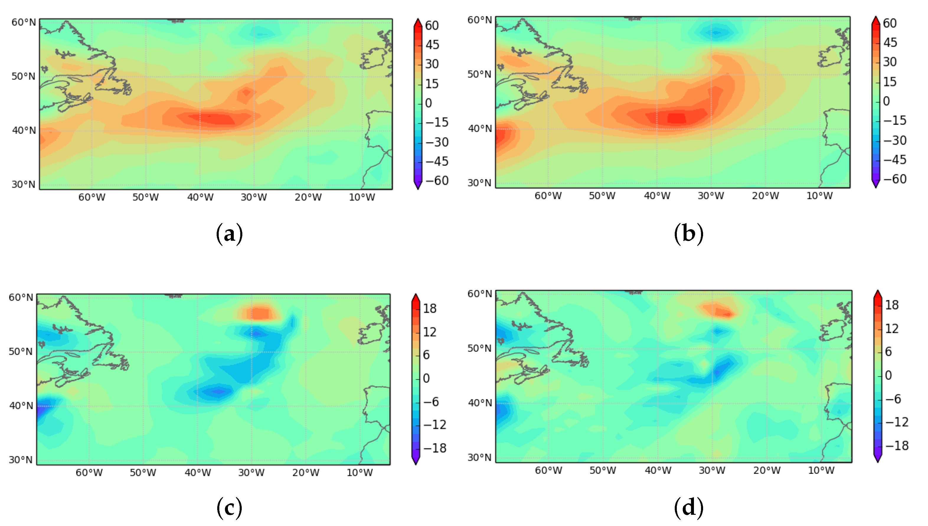
3.2. Comparison of Diagnostic and Model-Derived Ageotriptic Winds

Root mean square values of the geotriptic wind are about 21 ms 1 for this data, and root mean square values of the ageotriptic wind are about 6.3 ms 1 , giving a global averaged Rossby number of about 0.3. This would suggest a 10% expected error in the difference between the model wind and the total wind deduced from Equation (20). The actual global rms difference between the diagnosed wind and the model wind is 9.7 ms 1 in a overall rms wind of 22 ms 1 . The global rms difference between the calculated geostrophic wind and the model wind is 7.3 ms 1 .
To illustrate this, Figure 1 shows a mid-tropospheric zonal geotriptic wind calculated using Equations (10) and (11) from UM pressure and potential temperature fields. The area illustrated is the extratropical North Atlantic, so away from significant topography. It would be reasonable to expect the ageotriptic wind to be accurate over such an area. Figure 1 shows the ageotriptic wind calculated from Equation (20) and the difference between the UM wind and the geotriptic wind deduced from the pressure and temperature. There is a reasonable match between the two estimates of the ageotroptic wind, indicating that SGT theory is working reasonably accurately for the UM fields over the area chosen. The rms ageotriptic wind calculated from Equation (20) is 5.1 ms 1 over the area and level shown in Figure 1. The rms difference between the UM wind and the geotriptic wind is is 4.7 ms 1 in an overall rms wind of 22 ms 1 , so the proportional error in the geotriptic approximation is 20% rather than 45% globally. The rms difference between the two estimates of ageotriptic wind illustrated in Figure 1 is 3.8 ms 1 . If these fields are smoothed horizontally on the scale of the diagnostic grid, about 150 km, this difference reduces to 3.0 ms 1 . The correlation coefficient between the two estimates of the ageotriptic wind is 0.69 over the area and level illustrated. This both illustrates the applicability of the theory and the ability of the UM to reproduce it.
Figure 1 shows that the diagnosed ageotriptic wind is larger than the model value in some regions. This is typical of situations where the space or time scale is becoming too small for SGT theory to be accurate, and leads to the rms difference between the diagnosed wind and the model wind being no smaller than that between the calculated geotriptic wind and the model wind.

3.3. Use of a Modified Static Stability to Represent Latent Heat Release

In Section 2.3, it is shown that the latent heating resulting from maintenance of geotriptic balance in cloudy air can be deduced by solving Equation (20) with a modified static stability as in Equation (39). The resulting w can then be used in Equation (41) to deduce the latent heating. This can be compared with the temperature increments from the schemes representing cloud and precipitation, both convective and dynamic, in the UM.
The results are shown in Figure 2 for the same case as used in Figure 1. The area chosen is again the extratropical North Atlantic, so it can be expected that the vertical motion required to maintain geotriptic balance will be similar to that generated by the UM, and that precipitation processes, which generate most of the latent heating, will be strongly linked to the vertical velocity. In the first two panels, the vertical velocity w diagnosed from Equation (20) with Equation (39) is compared with that directly output from the UM. As in the comparison of ageotriptic winds in Figure 1, there is reasonable agreement. Comparing with Figure 1a, which shows the position of the strongest zonal winds, we see that there is systematic upward motion at the downstream end of the region of strongest zonal winds, and downward motion in the centre and rearward parts of this region. This is consistent with standard synoptic experience. The diagnosed vertical velocity has more coherent large scale structure, while the direct model output includes more small scale features, as would be expected. In the second pair of panels, the latent heating deduced from Equation (41) is compared with the temperature increments from the large-scale cloud scheme and the convection scheme combined. There is a strong correspondence between the diagnosed latent heating and the diagnosed vertical motion, as would be expected from Equation (39). The correspondence between the model vertical motion and the model latent heating does not look as strong. However, the correlation coefficient between them for the plotted area and level is again 0.69. The visual mismatch is primarily because there is no latent heating in areas of downward motion. The diagnostic procedure will generate latent cooling in cloudy air, but this would result in rapid dissipation of the cloud and not correspond to significant latent cooling in the UM.

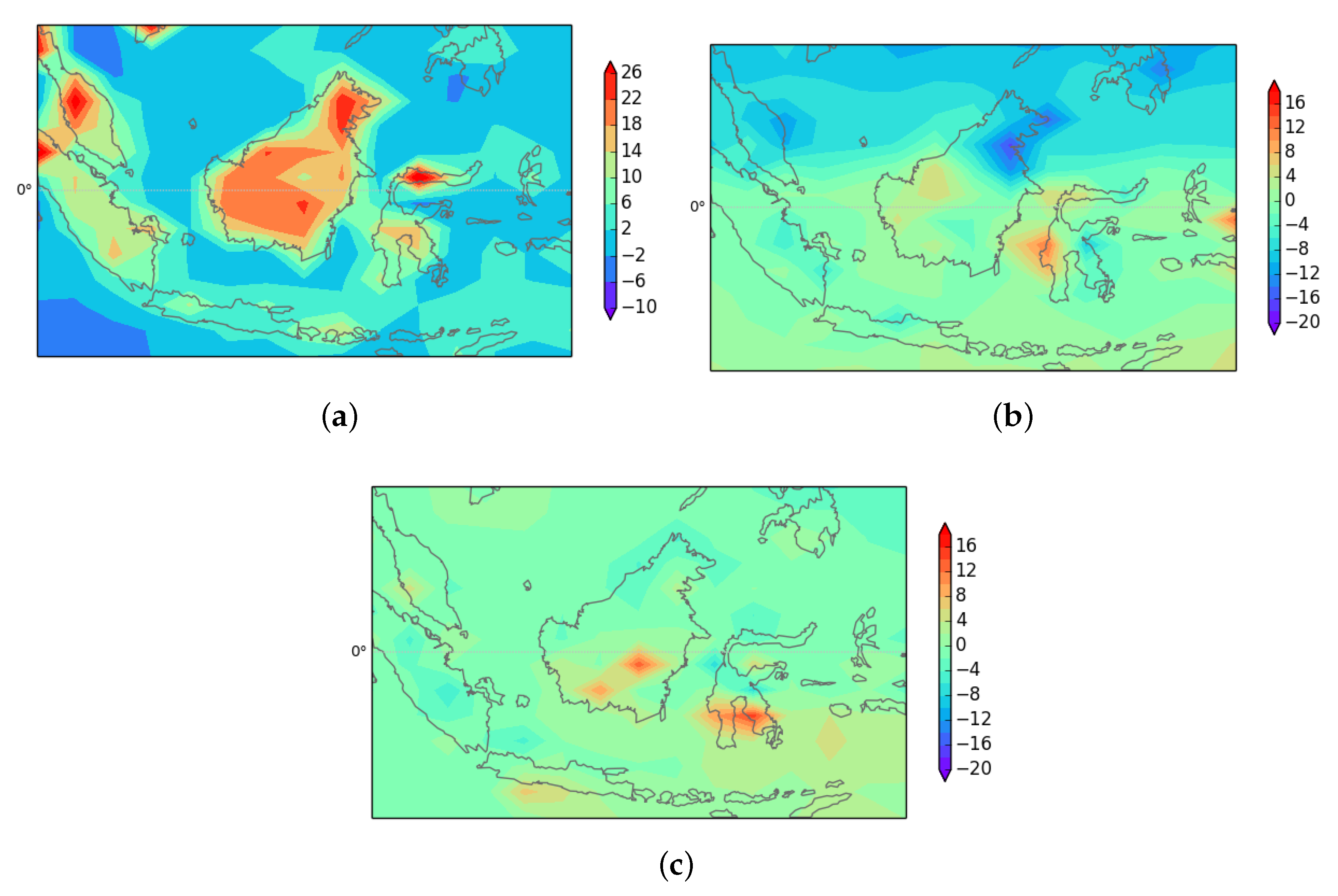
3.4. Effect of Tropical Heating on the Subtropical Jet

The diagnostic procedure can be applied using artificial physical forcing as well as that derived from the model. There has been considerable interest in the effect of tropical heating on the extratropical circulation. An example is the paper by Matthews et al. [30], where time dependent heating deduced from reanalyses is used to determine the response to forcing of a simple general circulation model (GCM) using a climatological mean state. This is compared with the observed evolution deduced from satellite data.
The diagnostic presented here calculates the “instant” response of the geostrophic flow to forcing at a particular time. It is thus easiest to compare it with the earlier study of [22]. In that paper, the forcing was maintained over a long timescale, and an actual atmospheric state as well as a climatological state could be used to determine the response to the forcing. The atmospheric state was maintained in time by using an artificial forcing term. We apply a forcing similar to [22] and calculate the instant geostrophic response to this forcing using the atmospheric state illustrated in the rest of the paper. In [22], Figure 17c shows the divergent response to the forcing, which is set up very quickly. This should be reproduced by the diagnostic. Figure 18c also shows a significant downstream response at about 30 N in the subtropical jet after five days. Since Figure 17c shows that the divergent response does not propagate much downstream, the formula for the source term plotted in Figure 18c shows that this must represent a perturbation vorticity. Thus, in our diagnostic, we look for a localised perturbation to the geotriptic flow in the subtropical jet, which would then propagate downstream over the five-day period illustrated by Jin et al. [22].
The heating in the mid troposphere is illustrated in Figure 3a. It is centred on the dateline as in [22], Figure 17c. The heating extends through the troposphere. The zonal geostrophic wind is shown in Figure 3b in the upper troposphere, noting that strong filtering has been applied near the equator to eliminate values for which SGT theory is inappropriate. The diagnosed zonal geostrophic wind tendency is shown in Figure 3c. This peaks at the same longitude as the forcing, so would propagate the jet forwards. The values peak at about 0.5 K day 1 . If this is applied over 15 days, this gives a similar impact to that shown in Figure 12a of [22]. There are also impacts at lower latitudes, but these are not likely to be physically correct as they are outside the validity of SGT.
The reason for the strong interaction with the subtropical jet can be seen in Figure 3d. This plots the second diagonal element of the matrix BQ defined in Equations (17) and (21). In the absence of the non-trivial model state this would take the value f 2 , about 0 . 5 × 10 8 at 30 N. It can be seen that on the southern flank of the jet, where there is strong anticyclonic shear, the values drop to well below this. The effect can be seen from Equation (20). If the matrix Q has a small eigenvalue, there will be a very strong response to forcing in this direction, so that in the present case there is a very efficient transfer of information from the heating to the subtropical jet. Comparing Figure 3a,c shows that the largest impact is to the west of the forcing longitude, where the matrix coefficient is smallest. The diagnostic can thus pick up sensitivity of the response to forcing to the structure of the basic state, which is a topic of wide interest.

3.5. Effect of Boundary Layer Heating

A feature of the diagnostic procedure is the inclusion of a proper treatment of the boundary layer. As shown in Equation (35), the boundary layer heating projects strongly onto the temperature, as the vertical motion is suppressed near the surface. This heating will also allow a horizontal temperature gradient to develop in the boundary layer. Since there is no horizontal pressure gradient above the boundary layer, hydrostatic balance will generate a heat low near the surface, resulting in convergence of the geotriptic wind which flows down the pressure gradient. Hence, upward motion will be generated at the top of the boundary layer. This effect forms part of the explanation of the heat lows that often form over tropical land masses [31].
This is particularly important in the tropics, where it allows representation of the return circulation consistent with the upward motion in the deep tropics. The example shown in Figure 4 illustrates the response to boundary layer heating over Borneo. The local time is around 1000 (0200UTC). There is strong convergence over both Borneo and Celebes to the east, leading to upward motion (not shown), and also anticyclonic rotation.

4. Discussion

The paper has developed a diagnostic procedure based on semi-geotriptic theory that can be applied successfully to data from a comprehensive global model. It is necessary to filter the data to large horizontal scales, particularly in the tropics, as expected. This means that it can be used to extract the “balanced” response to forcing, either by the model dynamics and physics, or artificially imposed forcing. The first example shows that the SGT approximation gives results which match the large-scale behaviour of the UM sufficiently closely to be useful. In particular, the predicted ageostrophic flow correlates quite well with the UM’s ageostrophic flow. Greater accuracy cannot realistically be expected given the wide range of scales and forcing mechanisms present in real and model-simulated flow. An alternative view is to say that the UM appears to reproduce the balanced response to forcing as calculated by the diagnostic.
The diagnostic calculates the large-scale response of the atmosphere to forcing, and thus allows studying the effect of both changes to the forcing and changes to the background flow. This will contribute to the understanding of large-scale circulation patterns, such as monsoons. In particular, it should aid the study of systematic errors, which usually have a large-scale signal. The predicted circulation is strongly dependent on the model state, so that errors in the resulting circulation can come from errors in the model state as well as errors in the forcing. In this application, the results of the diagnostic procedure would need to be averaged over a large number of cases, so that the noise created by using data on the borderline for applicability of SGT would be filtered out. The second example supports this by showing that much of the extratropical precipitation signal can be reproduced using the diagnosed vertical motion and the cloud fraction. This will help in identifying the causes of systematic errors in precipitation. The third example shows that the effect of tropical–extratropical interaction is strongly dependent on the background state assumed; the causes of errors in this could be distinguished by replacing the model state with a reanalysis, while still using the same forcing. The final example shows the leading order effect of boundary layer forcing on the circulation, again allowing the causes of systematic errors to be identified.

Funding

This research received no external funding.

Acknowledgments

The author would like to thank Michael Haigh, a Ph.D. student at Imperial College, for careful reading of the manuscript, and three anonymous referees for their constructive comments.

Conflicts of Interest

The author declares no conflict of interest.

Abbreviations

The following abbreviations are used in this manuscript:
GCMGeneral Circulation Model
SEESawyer–Eliassen equation
SGsemi-geostrophic
SGTsemi-geotriptic
UMUnified Model
WTGWeak Temperature Gradient

References

  1. Brown, A.; Milton, S.; Cullen, M.; Golding, B.; Mitchell, J.; Shelly, A. Unified modeling and prediction of weather and climate: A 25-year journey. Bull. Am. Meteorol. Soc. 2012, 93, 1865–1877. [Google Scholar] [CrossRef]
  2. Martin, G.M.; Milton, S.F.; Senior, C.A.; Brooks, M.E.; Ineson, S.; Reichler, T.; Kim, J. Analysis and reduction of systematic errors through a seamless approach to modeling weather and climate. J. Clim. 2010, 23, 5933–5957. [Google Scholar] [CrossRef]
  3. Sobel, A.H.; Nilsson, J.; Polvani, L.M. The weak temperature gradient approximation and balanced tropical moisture waves. J. Atmos. Sci. 2001, 58, 3650–3665. [Google Scholar] [CrossRef]
  4. Beare, R.J.; Cullen, M.J.P. Diagnosis of boundary-layer circulations. Philos. Trans. R. Soc. A 2013, 371, 20110474. [Google Scholar] [CrossRef] [PubMed]
  5. Cullen, M.J.P. A Mathematical Theory of Large-Scale Atmospheric Flow; Imperial College Press: London, UK, 2006; 259p, ISBN 1-86094-518-X. [Google Scholar]
  6. Malardel, S.; Thorpe, A.J.; Joly, A. Consequences of the geostrophic momentum approximation on barotropic instability. J. Atmos. Sci. 1997, 54, 103–112. [Google Scholar] [CrossRef]
  7. Cullen, M.J.P.; Mawson, M.H. An idealised simulation of the Indian monsoon using primitive-equation and quasi-equilibrium models. Quart. J. R. Meteorol. Soc. 1992, 118, 153–164. [Google Scholar]
  8. Eliassen, A. The quasi-static equations of motion with pressure as independent variable. Geofys. Publ. 1950, 17, 3–43. [Google Scholar]
  9. Charney, J.G. On the scale of atmospheric motions. Geofys. Publ. 1948, 17, 4–17. [Google Scholar]
  10. Phillips, N.A. Geostrophic motion. Rev. Geophys. 1963, 1, 123–176. [Google Scholar] [CrossRef]
  11. Eliassen, A. Geostrophy. Quart. J. R. Meteorol. Soc. 1984, 110, 1–12. [Google Scholar] [CrossRef]
  12. Hoskins, B.J. The mathematical theory of frontogenesis. Ann. Rev. Fluid Mech. 1982, 14, 131–151. [Google Scholar] [CrossRef]
  13. Cullen, M.J.P.; Douglas, R.J.; Roulstone, I.; Sewell, M.J. Generalised semi-geostrophic theory on a sphere. J. Fluid Mech. 2005, 531, 123–157. [Google Scholar] [CrossRef]
  14. Cullen, M.J.P. Analysis of the semi-geostrophic shallow water equations. Phys. D 2008, 237, 1461–1465. [Google Scholar] [CrossRef]
  15. Cheng, J.; Cullen, M.J.P.; Feldman, M. Semi-geostrophic system with variable Coriolis parameter. Arch. Ration. Mech. Anal. 2016, 1–58. [Google Scholar] [CrossRef]
  16. Schubert, W.H. Semi-geostrophic theory. J. Atmos. Sci. 1985, 42, 1770–1772. [Google Scholar] [CrossRef]
  17. Xu, Q. Extended Sawyer-Eliassen Equation for Frontal Circulations in the Presence of small Viscous Moist Symmetric Stability. J. Atmos. Sci. 1989, 46, 2671–2683. [Google Scholar] [CrossRef]
  18. Cullen, M.J.P. Semigeostrophic solutions for flow over a ridge. Quart. J. R. Meteorol. Soc. 2007, 133, 491–501. [Google Scholar] [CrossRef]
  19. Thorpe, A.J.; Pedder, M.A. The semi-geostrophic diagnosis of vertical motion. II: Results for an idealized baroclinic wave life cycle. Quart. J. R. Meteorol. Soc. 1999, 125, 1257–1276. [Google Scholar]
  20. Wernli, H.; Fehlmann, R.; Luthi, D. The Effect of Barotropic Shear on Upper-Level Induced Cyclogenesis: Semigeostrophic and Primitive Equation Numerical Simulations. J. Atmos. Sci. 1998, 55, 2080–2094. [Google Scholar] [CrossRef]
  21. Ragone, F.; Badin, G. A study of surface semi-geostrophic turbulence: Freely decaying dynamics. J. Fluid Mech. 2016, 792, 740–774. [Google Scholar] [CrossRef]
  22. Jin, F.; Hoskins, B.J. The direct response to tropical heating in a baroclinic atmosphere. J. Atmos. Sci. 1995, 52, 307–319. [Google Scholar] [CrossRef]
  23. Schubert, W.H.; Ciesieleski, P.E.; Stevens, D.E.; Kuo, H.-C. Potential vorticity modelling of the ITCZ and the Hadley circulation. J. Atmos. Sci. 1991, 48, 1493–1509. [Google Scholar] [CrossRef]
  24. Wood, N.; Staniforth, A.; White, A.; Allen, T.; Diamantakis, M.; Gross, M.; Melvin, T.; Smith, C.; Vosper, S.; Zerroukat, M.; et al. An inherently mass-conserving semi-implicit semi-Lagrangian discretization of the deep-atmosphere global nonhydrostatic equations. Quart. J. R. Meteorol. Soc. 2014, 140, 1505–1520. [Google Scholar] [CrossRef]
  25. White, A.A.; Hoskins, B.J.; Roulstone, I.; Staniforth, A. Consistent approximate models of the global atmosphere: Shallow, deep, hydrostatic, quasi-hydrostatic and non-hydrostatic. Quart. J. R. Meteorol. Soc. 2005, 131, 2081–2108. [Google Scholar] [CrossRef] [Green Version]
  26. Beare, R.J.; Cullen, M.J.P. Validating weather and climate models at small Rossby numbers: Including a boundary layer. Quart. J. R. Meteorol. Soc. 2016, 142, 2636–2645. [Google Scholar] [CrossRef]
  27. Holton, J.R.; Hakim, G.J. An Introduction to Dynamic Meteorology, 5th ed.; Academic Press: Cambridge, MA, USA, 2013; ISBN 978-0-12-384866-6. [Google Scholar]
  28. Booth, J.F.; Polvani, L.; O’Gorman, P.A.; Wang, S. Effective stability in a moist baroclinic wave. Atmos. Sci. Lett. 2015, 16, 56–62. [Google Scholar] [CrossRef]
  29. Hinch, E.J. Perturbation Methods; Cambridge University Press: Cambridge, UK, 1991; ISBN 0-521-37310-7. [Google Scholar]
  30. Matthews, A.J.; Hoskins, B.J.; Masutani, M. The global response to tropical heating in the Madden-Julian oscillation during the northern winter. Quart. J. R. Meteorol. Soc. 2004, 130, 1991–2011. [Google Scholar] [CrossRef] [Green Version]
  31. Smith, R.K.; Spengler, T. The dynamics of heat lows over elevated terrain. Quart. J. R. Meteorol. Soc. 2011, 137, 250–263. [Google Scholar] [CrossRef]
Figure 1. Zonal component of wind at 4000 m, units ms 1 : (a) direct UM output; (b) geotriptic wind calculated from Equation (10); (c) ageotriptic wind from Equation (20); and (d) ageotriptic wind from UM output.
Fluids 03 00072 g001
Figure 2. Vertical velocity at 4000m, units ms 1 : (a) directly output from UM; (b) calculated from Equation (20) with heating rates at 4000 m, units K day 1 ; (c) combined heating from precipitation schemes in UM; and (d) latent heating deduced as in Section 2.3 (see text).
Fluids 03 00072 g002
Figure 3. (a) Heating rate at 4000 m, units K day 1 ; (b) zonal geostrophic wind units ms 1 at 11,500 m; (c) diagnosed zonal geostrophic wind tendency at 11,500 m, units ms 2 ; and (d) (22) coefficient of BQ’ matrix, Equation (21), at 11,500 m, units 10 8 × s 2 .
Fluids 03 00072 g003
Figure 4. Diagnostics calculated over a region 10 S to 10 N and 100 E to 130 E at 80 m height above the surface: (a) Boundary layer heating, units K day 1 ; (b) total zonal wind calculated from Equation (20); and (c) total meridional wind calculated from Equation (20).
Fluids 03 00072 g004

