Evolve Filter Stabilization Reduced-Order Model for Stochastic Burgers Equation

Abstract

In this paper, we introduce the evolve-then-filter (EF) regularization method for reduced order modeling of convection-dominated stochastic systems. The standard Galerkin projection reduced order model (G-ROM) yield numerical oscillations in a convection-dominated regime. The evolve-then-filter reduced order model (EF-ROM) aims at the numerical stabilization of the standard G-ROM, which uses explicit ROM spatial filter to regularize various terms in the reduced order model (ROM). Our numerical results are based on a stochastic Burgers equation with linear multiplicative noise. The numerical result shows that the EF-ROM is significantly better than G-ROM.

1. Introduction

Many important scientific and engineering applications require repeated numerical simulations of large and complex dynamical systems with high computational cost [1,2,3,4]. The high-fidelity simulation of such large-scale dynamic system is so expensive that it requires a lot of computational resources. Reduced order models (ROMs), therefore, have been successfully introduced to reduce the expensiveness of the numerical simulations. ROMs aim to find a low-dimensional approximation to the full order model (FOM) with orders of magnitude reduction in computational cost and high accuracy. The low-dimensional subspace is constructed through proper orthogonal decomposition (POD). The standard Galerkin projection based reduced order model (G-ROM) is obtained by projecting the FOM to the low-dimensional subspace. G-ROM is successful across a range of disciplines; however, its use in convection-dominated flows has been hampered by the projection instability. The main reason is that the Galerkin projection does not preserve the stability properties of the Navier–Stokes equation since the projection can lead to an unstable reduced order model (ROM) for a stable fixed point. Typically, it leads to a marginally stable ROM for a strongly stable solution [2,4,5,6]. This instability, usually in the form of unphysical numerical oscillations, yields inaccurate results for nonlinear dynamic systems. To mitigate the spurious numerical oscillations, various stabilized reduced order models (ROMs) have been introduced (see [3,7,8,9,10,11,12]). One popular strategy is the ROM closure modeling which models the lost information in the truncation of the POD basis; many ROMs can be found in [3,12,13,14,15,16,17]. Another approach is the regularization, which uses explicit spatial filtering to regularize the standard G-ROM and increase the numerical stability of the ROM approximation. The recent development of regularized reduced-order model method for deterministic systems has been introduced in [18,19].

Reduced order models (ROMs) for systems involving stochastic process have gained increasing attention recently [20,21,22]. The development of ROMs for partial differential equations (PDEs) subject to random inputs acting on the boundary and PDEs with random coefficients have been considered intensely in various contexts [23,24,25]. Some works have been done for ROMs for evolutionary PDEs driven by stochastic processes [26,27]. Leray-regularization reduced order model (L-ROM) for the stochastic system with Brownian motions was in troduced in [28].

In this paper, we address the instability issue of standard G-ROM for nonlinear stochastic PDEs by using regularization. Motivated by [28], we introduce another regularized ROM, evolve-then-filter (EF-ROM), for stochastic PDEs (SPDEs) that are of relevance to fluid dynamics as used in [28]. The main purpose is to numerically investigate the evolve-then-filter regularization ROM (EF-ROM) for the stabilization of the G-ROM within a simple setting, a stochastic Burgers equation (SBE) driven by linear multiplicative noise. In [28], it has been shown that the spurious oscillations in G-ROM persist as the noise is turned on, and the oscillations worsen as the noise amplitude increases. The numerical test of EF-ROM shows that it gives more accurate modeling of the SBE dynamics by reducing the oscillations of the G-ROM with a low dimensional approximation.

The rest of the paper is organized as follows: in Section 2, we briefly describe the SBE to be used in our numerical experiment. In Section 3, we provide details about the derivation of the corresponding G-ROM and EF-ROM based on proper orthogonal decomposition. In Section 4, we introduce the evolve-then-filter algorithm for the G-ROM. In Section 5, we present our numerical investigation of the EF-ROM. Finally, we outline conclusions and potential future research directions in Section 6.

2. Stochastic Burgers Equation (SBE)

SPDEs driven by linear multiplicative noise arise in various contexts, including turbulence theory, non-equilibrium phase transitions, or simply the modeling of parameter disturbance [29,30,31,32]. We use the stochastic Burgers equation (SBE) as the first numerical investigation of our model. We claim that the proposed new model can be applied to a wide scope of SPDEs. In this section, we introduce the SBE with linear multiplicative noise and its numerical scheme that we used to collect the snapshot data:

$$\begin{array}{c}\mathrm{d}u=\left(\nu u_{xx}-u{u}_x\right)\mathrm{d}t+\sigma u\circ \mathrm{d}{W}_t,\hfill \\ u(0,t)=u(1,t)=0,t\ge 0,\hfill \\ u(x,0)=u_0(x),x\in (0,1),\hfill \end{array}$$

(1)

where $W_t$ is a two-sided one-dimensional Wiener process, $\sigma$ measures the “amplitude” of the noise, and $\nu$ is a positive diffusion coefficient. In stochastic differential equations (SDE), there are two types of equations: Stratonovich SDE and Ito SDE. One can use Ito’s formula to find a translation between Ito and Stratonovich SDE. Since the noise is a representation of part of a continuous fluid dynamical system, the multiplicative noise term $\sigma u\circ \mathrm{d}{W}_t$ is understood in the sense of Stratonovich [33]. The initial condition $u_0(x)=1$ if $x\in (0.05,0.55)$ and $u_0(x)=0$, otherwise. Detailed mathematical definition of the initial function can be found in [28].

2.1. Numerical Discretization of SBE

In our numerical experiment, the SBE Equation of Label (1) is solved by a semi-implicit Euler scheme as given in Section 6.1 in [27]. We present the numerical discretization scheme below. Other numerical approximation methods of nonlinear SPDEs can be found in [26,34,35,36,37,38].

The nonlinearity $u{u}_x={(u^2)}_x/2$ and the noise term $\sigma u\circ \mathrm{d}{W}_t$ are discretized explicitly for each time step, while the other terms are treated implicitly. Thus, we can get the following semi-implicit discretization scheme:

$$\begin{array}{c}\hfill u_i^{n+1}-u_i^n=\left(\nu u_{i,xx}^{n+1}+\frac{{\sigma }^2}{2}{u}_i^n-\frac{1}{2}{(u_i^n)}_x^2\right)\Delta t+\sigma {\zeta }_n{u}_i^n\sqrt{\Delta t},\end{array}$$

(2)

where $u_i^n$ is the discrete approximation of $u(i\Delta x,n\Delta t)$, $\Delta x$ and $\Delta t$ are the mesh size of the spatial discretization and the time step, respectively. The second derivative is discretized using the standard second-order central difference approximation given by

$$u_{i,xx}^n=\frac{u_{i-1}^n-2u_i^n+u_{i+1}^n}{{(\Delta x)}^2};{(u_i^n)}_x^2=\frac{{(u_{i+1}^n)}^2-{(u_i^n)}^2}{\Delta x},i\in \{1,\cdots ,N_x-2\},$$

where the boundary conditions are $u_0^n=u_{N_x-1}^n=0$, and $N_x$ is the total number of grid points of the spatial discretization in $[0,1]$. The ${\zeta }_n$ are random variables drawn independently from a normal distribution $\mathcal{N}(0,1)$. The additional drift term ${\sigma }^2{u}_j^n/2$ in Label (2) is the conversion of the Stratonovich noise term $\sigma u\circ \mathrm{d}{W}_t$ into Itô form.

3. Reduced Order Modeling

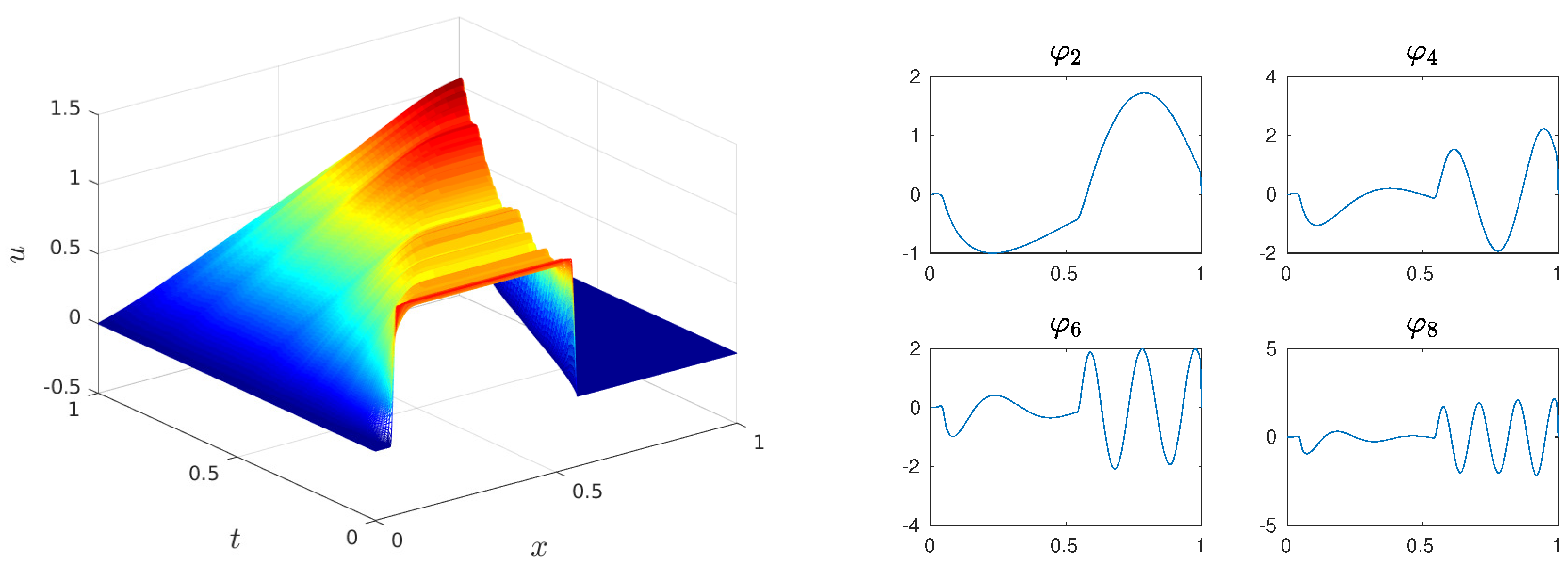
3.1. Proper Orthogonal Decomposition

POD is one of the most popular data-driven reduced order modeling methods, which we exclusively use to generate the ROM basis in this paper. We briefly describe the POD in this section. We note, however, that other ROM bases (e.g., the dynamic mode decomposition (DMD)) could be used. For more details, the reader is referred to [1,39,40,41]. The POD starts with the snapshots $\{{\mathit{u}}^0,\dots ,{\mathit{u}}^{N_s}\}$, which are numerical approximations of the SBE at $N_s$ different time instances. The POD seeks a low-dimensional space ${\mathit{X}}^r:=span\{{\mathbf{\phi }}_1,\dots ,{\mathbf{\phi }}_r\}$ that approximates the snapshots optimally with respect to $L^2$-norm.

Consider an ensemble of snapshots $\mathcal{R}:=span\left\{{\mathit{u}}^0,\dots ,{\mathit{u}}^{N_s}\right\}$, which is a collection of velocity data from either numerical simulations or experimental observations at time $t_i=i\Delta t$, $i=0,\dots ,N_s$. The POD basis ${\{\mathbf{\phi }\}}_i$ comes from the minimization problem:

$$min\frac{1}{N_s+1}\sum _{\ell =0}^{N_s}{∥\mathit{u}(·,t_{\ell })-\sum _{j=1}^r(\mathit{u}(·,t_{\ell }),{\mathbf{\phi }}_j(·)){\mathbf{\phi }}_j(·)∥}^2$$

(3)

subject to the conditions $({\mathbf{\phi }}_j,{\mathbf{\phi }}_i)={\delta }_{ij},1\le i,j\le r$, and ${\delta }_{ij}$ is the Kronecker delta. The minimization problem results in the eigenvalue problem $K{\mathit{z}}_j={\lambda }_j{\mathit{z}}_j,\mathrm{for}j=1,\dots ,r,$ where $K\in {\mathbb{R}}^{(N_s+1)\times (N_s+1)}$ is the snapshot correlation matrix with entries ${\displaystyle K_{k\ell }=\frac{1}{N_s+1}\left(\mathit{u}(·,t_{\ell }),\mathit{u}(·,t_k)\right)}$ for $\ell ,k=0,\dots ,N_s$, ${\mathit{z}}_j$ is the j-th eigenvector, and ${\lambda }_j$ is the associated eigenvalue. It can be shown that the POD basis functions are given by ${\mathbf{\phi }}_j(·)=\frac{1}{\sqrt{{\lambda }_j}}{\sum }_{\ell =0}^{N_s}{({\mathit{z}}_j)}_{\ell }\mathit{u}(·,t_{\ell }),1\le j\le r,$ ${({\mathit{z}}_j)}_{\ell }$ is the ℓ-th component of the eigenvector ${\mathit{z}}_j$. In addition, the following error formula holds from [42,43]:

$$\frac{1}{N_s+1}\sum _{\ell =0}^{N_s}{∥\mathit{u}(·,t_{\ell })-\sum _{j=1}^r{(\mathit{u}(·,t_{\ell }),{\mathbf{\phi }}_j(·))}_{\mathcal{H}}{\mathbf{\phi }}_j(·)∥}^2=\sum _{j=r+1}^d{\lambda }_j,$$

(4)

where d is the rank of the snapshot correlation matrix $K_{kl}$. Note that in many ROMs of fluid dynamics, snapshots matrix always assembled by subtracting the centering trajectory when generating the POD basis. That is, the fluctuations ${\mathit{u}}^{\prime }=\mathit{u}-\mathit{U}$, $\mathit{U}$ is the centering trajectory, are considered in the data matrix. For our numerical investigation, however, we do not use the centering trajectory approach for the simple one-dimension SBE case.

3.2. Galerkin Projection ROM (G-ROM)

The classic Galerkin projection based reduced order model is one of the most popular model reduction methods since it only requires computing the ROM operators from Galerkin projection at offline. The derivation of the POD Galerkin ROM (G-ROM) follows the standard Galerkin approximation procedure. For a given low-dimensional space ($r\sim \mathcal{O}(10)$), the approximation $u_r$ of the SBE solution u spanned by the POD basis:

$${\mathit{u}}_r(\mathit{x},t;\omega ):=\sum _{j=1}^r{a}_j(t;\omega ){\mathbf{\phi }}_j(\mathit{x}),$$

(5)

where the time-varying coefficients (ROM coefficients) ${\{a_j(t,\omega )\}}_{j=1}^r$ are determined by solving:

$$\left(\mathrm{d}{u}_r,{\mathbf{\phi }}_j\right)=\left(\nu {(u_r)}_{xx}-u_r{(u_r)}_x,{\mathbf{\phi }}_j\right)\mathrm{d}t+\sigma \left(u_r,{\mathbf{\phi }}_j\right)\circ \mathrm{d}{W}_t,j=1,\cdots ,r.$$

(6)

The above low dimensional dynamic system of Label (6) is called the Galerkin ROM equation of the stochastic Burgers equation (SBE). The general ROM dynamic system can be often written as

$$\begin{array}{c}\hfill \dot{\mathit{a}}=f(\mathit{a}).\end{array}$$

(7)

The ROM online computation involves time integration of system Label (7), which is carried out by using a standard Euler scheme [44]. The fully discretized G-ROM of SBE is as follows:

$$\begin{array}{c}\hfill {\mathit{a}}^{n+1}-{\mathit{a}}^n=\Delta tf({\mathit{a}}^n).\end{array}$$

(8)

The right-hand side of G-ROM can be written as

$$\begin{array}{cc}\hfill \Delta tf({\mathit{a}}^n)& =[-\nu \sum _{k=1}^r{a}_k^n\left({({\mathbf{\phi }}_k)}_x,{({\mathbf{\phi }}_j)}_x\right)+\frac{{\sigma }^2}{2}{a}_j^n\hfill \\ & +\sum _{k,l=1}^r{a}_k^n{a}_l^n\left({\mathbf{\phi }}_k{({\mathbf{\phi }}_l)}_x,{\mathbf{\phi }}_j\right)]\Delta t+\sigma {\zeta }_n{a}_j^n\sqrt{\Delta t},j=1,\cdots ,r,\hfill \end{array}$$

(9)

where ${\zeta }_n$ are random variables drawn independently from a normal distribution $\mathcal{N}(0,1)$. Note that other numerical discretization schemes can be used for the ROM integration of Label (7).

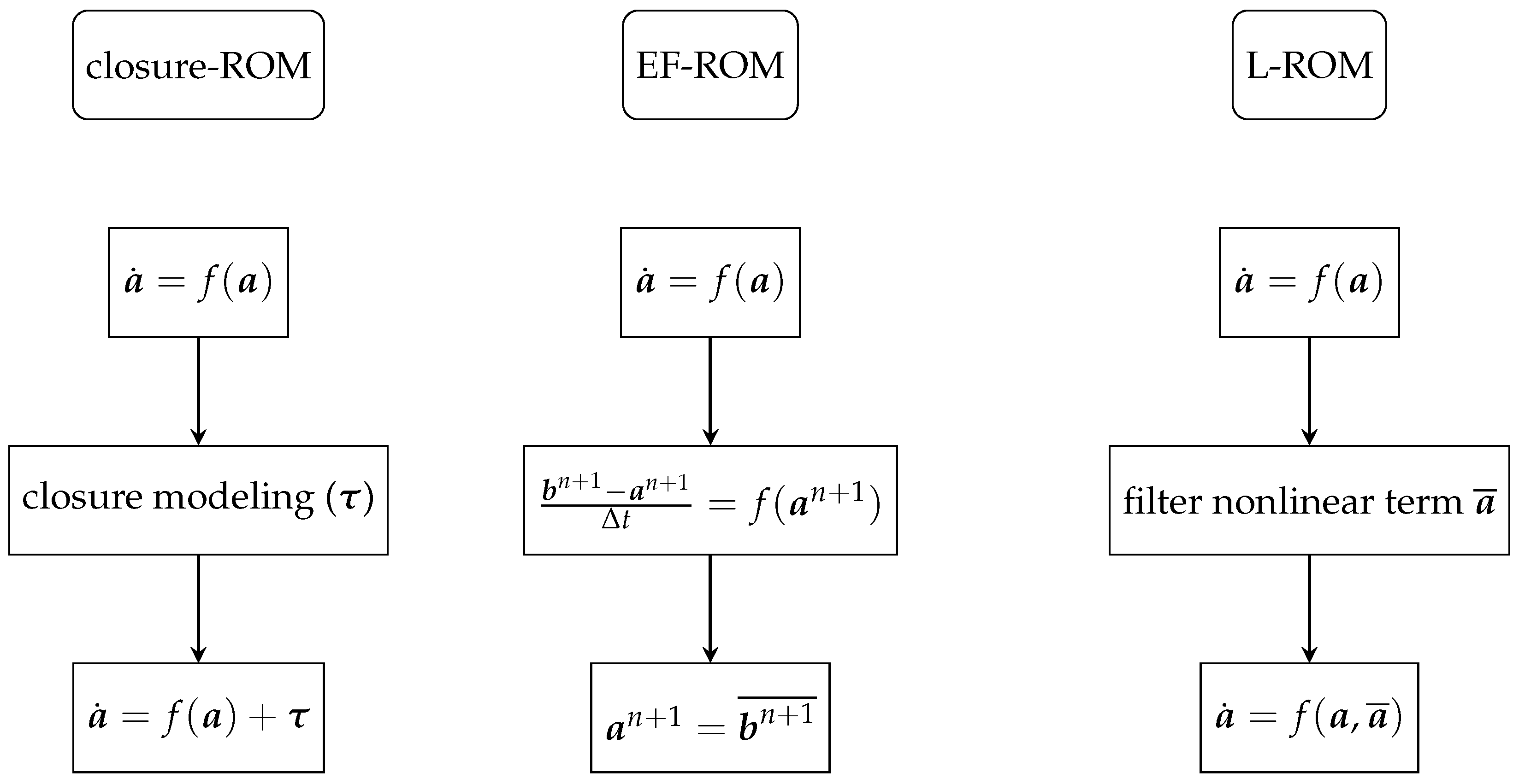
4. Evolve-Then-Filter Regularized ROM

The G-ROM is efficient and relatively accurate for many deterministic fluid flows. As mentioned before, however, G-ROM is inaccurate for convection-dominated flows because of the numerical instability. In this section, we introduce the EF-ROM regularization for the SBE to investigate potential improvement for numerical instability. This EF-ROM regularization based on POD spatial filtering to smooth the flow variables and increase the numerical stability of the model (see Section 4.1).

4.1. POD Differential Filter

We present details of the ROM spatial filtering (Differential Filter) in this section. Let $\delta$ be the radius of the DF. The POD differential filter (DF) is defined as, for a given ${\mathit{u}}^r\in {\mathit{X}}^r$, find ${\overline{\mathit{u}}}^r\in {\mathit{X}}^r$ such that

$$\begin{array}{c}\hfill \left(\right(I-{\delta }^2\Delta ){\overline{\mathit{u}}}^r,{\mathbf{\phi }}_j)=({\mathit{u}}^r,{\mathbf{\phi }}_j),\forall j=1,\dots r.\end{array}$$

(10)

Differential filters (DF) have been used in the simulation of convection-dominated flows with standard numerical methods [45,46]. The DF of Label (10) uses an explicit length scale $\delta$ (i.e., the radius of the filter) to eliminate the small scales (i.e., high frequencies) from the input. Indeed, the DF uses an elliptic operator to smooth the input variable. The DF also has a low computational overhead as it solves a linear system with a very small $r\times r$ matrix that is precomputed. Another advantage is ROM DF preserving incompressibility in the Navier-Stokes equation (NSE), since they are linear operators. In reduced order modeling, POD-DF was first used in [18]. In this paper, we apply POD-DF to the SBE system (1).

4.2. EF-ROM for SBE

The Evolve-Then-Filter model has been used as a numerical tool in the simulation of convection-dominated deterministic flows [47,48]. It has also been used to derive regularized ROMs (Reg-ROMs) for deterministic systems in [18,19]. We draw inspiration from the deterministic case and consider the evolve-then-filter ROM (EF-ROM) constructed from the POD differential filter [19]. The EF-ROM belongs to the wide class of stabilized ROMs [3,7,8,9,10,11,12,13,49,50]. The main difference between EF-ROM and the other stabilized ROMs is that EF-ROM increases the numerical stability of the model by using two-stage regularization with explicit spatial filtering, which is a relatively new concept in the ROM field [12,18]. Other ROMs use closure modeling both physically and mathematically. The construction of the EF-ROM to the stochastic problem in Label (1) contains two steps: first, evolve the ROM dynamic system as the same in G-ROM; second, filter the small scales from evolved trajectory to smooth the solution. There is only one crucial difference in its derivation compared to the derivation of the G-ROM as outlined in Section 3.2, which consists of applying POD-DF after evolving the dynamic system.

The r-dimensional EF-ROM approximation $u_r$ of the SBE solution u takes the form Label (5). The time-varying coefficients ${\{a_j(t,\omega )\}}_{j=1}^r$ are determined by solving:

$$\begin{array}{ccc}\hfill \left(w_r^{n+1}-u_r^n,{\mathbf{\phi }}_j\right)& =& \left(\nu {(u_r^n)}_{xx}-u_r^n{(u_r^n)}_x,{\mathbf{\phi }}_j\right)\mathrm{d}t+\sigma \left(u_r^n,{\mathbf{\phi }}_j\right)\circ \mathrm{d}{W}_t,j=1,\cdots ,r.\hfill \end{array}$$

(11)

$$\begin{array}{ccc}\hfill u_r^{n+1}& =& \overline{w_r^{n+1}}.\hfill \end{array}$$

(12)

The first “evolve” step in the EF-ROM Label (11) is just one step of the time discretization of the standard G-ROM in Label (9). The “filter” step in the EF-ROM consists of filtering of the intermediate solution obtained in the previous step:

$$\begin{array}{c}\hfill \left(\left(I-{\delta }^2\Delta \right)\overline{w_r^{n+1}},{\mathbf{\phi }}_j\right)=(w_r^{n+1},{\mathbf{\phi }}_j),\forall j=1,\dots r,\end{array}$$

(13)

$$\overline{w_r^{n+1}}(t,x;\omega )\equiv \sum _{k=1}^r{\overline{b}}_k(t;\omega ){\mathbf{\phi }}_k(\mathit{x}).$$

(14)

This could give us the following linear system:

$$\begin{array}{c}\hfill (M_r+{\delta }^2{S}_r)\overline{\mathit{b}}=M_r\mathit{b},\end{array}$$

(15)

where $M_r=({\mathbf{\phi }}_i,{\mathbf{\phi }}_j)$ and $S_r=(\nabla {\mathbf{\phi }}_i,\nabla {\mathbf{\phi }}_j)$ are the POD mass matrix and stiffness matrix, respectively, and $\overline{b}$ is the filtered POD coefficient. The r-dimensional EF-ROM for SBE (1) is given by:

$$\begin{array}{ccc}\hfill b_j^{n+1}-a_j^n& =& \left[-\nu \sum _{k=1}^r{a}_k^n\left({({\mathbf{\phi }}_k)}_x,{({\mathbf{\phi }}_j)}_x\right)+\sum _{k,l=1}^r{a}_k^n{a}_l^n\left({\mathbf{\phi }}_k{({\mathbf{\phi }}_l)}_x,{\mathbf{\phi }}_j\right)\right]\Delta t+\sigma {\zeta }_n{a}_j^n\circ \sqrt{\Delta t},\hfill \end{array}$$

(16)

$$\begin{array}{ccc}\hfill a_j^{n+1}& =& \overline{b_j^{n+1}},\hfill \end{array}$$

(17)

where $j=1,\cdots ,r$. As mentioned in Section 4, a forward Euler time discretization was used in Label (11), but other time discretizations are possible [51].

Unlike the Leray-ROM (L-ROM) [28,52], which only filters the nonlinear term, the EF-ROM filters all the dynamics of the coefficients after the “evolve” step. Some numerical analysis regards these two methods for standard turbulent flows have been studied in [48]. A full comparison of the Reg-ROMs for deterministic systems was studied in [19]. We emphasize that a numerical comparison of the EF-ROM and L-ROM for stochastic Burgers system is beyond the scope of this paper. A further study with more discussions and complex stochastic systems will be investigated for future research. Figure 1 shows the flowchart of EF-ROM, L-ROM and the general framework of stabilized closure models.

5. Numerical Results

In this section, we present our numerical results for the EF-ROM and compare it with the standard G-ROM. The data that we used to construct our ROM is generated by the method described in Section 2.1 with the diffusion coefficient $\nu =0.001$, $\Delta t={10}^{-4}$ and $N_x=1025$ so that $\Delta x\approx 9.8\times {10}^{-4}$. We collected 101 equally spaced snapshots on the time interval $[0,1]$ and used the method of snapshots to compute the POD bases. The solution field and a few POD basis functions are shown in Figure 2 for illustration purposes.

Even though the first few POD modes extract the most dominant percentage of energy (see

Table 1. The energy captured by the first few proper orthogonal decomposition (POD) bases from stochastic Burgers equation (SBE) data with $\sigma =0.3$.

No. of Basis	Energy
2	91.38%
4	97.20%
6	98.46%
8	99.02%

), the corresponding G-ROM generates very high numerical oscillations, which yield inaccurate results. This can be observed from the reconstructed ROM solution field in Figure 3. For the SBE problem studied here, as we said before, the purpose of EF-ROM is to alleviate the spurious oscillations generated in standard G-ROM. We can see from Figure 3 that, indeed, the oscillations are significantly reduced in the spatio-temporal numerical reconstruction by EF-ROM resulting in a better approximation to the original SBE system. In addition, note that, as the dimension of the ROM increases, the overall performance of both ROMs improves (see Figure 3). This behavior is expected since increasing dimension r increases the amount of energy used to the dynamic system of ROM, which accurately approximates the SBE.

The parameter $\delta$ is the filter length of the POD-DF in Label (10) that can determine the size of filtered spatial scales in the ROM dynamic system (13). Large $\delta$ value means filtering too much of the spatial field, which generates very bad results, while small value (identical to zero) means filtering nothing just like the G-ROM. The optimal value ($\delta$) is defined mathematically by minimizing the $L^2$-error of the EF-ROM in numerical approximating the SBE’s spatio-temporal field,

$$\underset{\delta }{min}{\parallel \mathit{u}-{\mathit{u}}_r(x,t,r,\delta ,\sigma ,{\zeta }_n)\parallel }^2.$$

(18)

The noise ($\sigma$), dimension r and random variable ${\zeta }_n$ in the numerical algorithm (16) can change the performance of the different $\delta$. All of these parameters have to be appropriately calibrated to reach a good performance. We fix $\sigma ,r$ to reduce the numerical efforts. The “optimal” $\delta =0.0011$ is reached when $\sigma =0$ for $r=4,6,8$, and we fix this $\delta$ for all the numerical (statistical) experiments.

Another comparison of the two ROMs can be made by looking at the time evolution of the projected coefficients onto each POD mode. The dynamics of POD coefficients can reveal how the model performs from the magnitude and the trajectory of each coefficient. Figure 4 shows the evolution of POD coefficients corresponding to each POD basis. The two ROMs are performed quite well and similarly for the leading coefficients $a_2$ and $a_3$. For high-frequency modes, however, G-ROM models badly about the dynamics in terms of magnitude, whereas EF-ROM generates a closer trajectory to SBE (see coefficients $a_4-a_8$ in Figure 4). It is interesting to note that the EF-ROM leads to a slight deterioration on the dynamic of first mode $a_1$ (see Figure 4). This deterioration exists even if the optimal $\delta$ is reached. The conjecture is that the DF spatial filtering affects this little deterioration. As the first POD mode contains the most dominant energy, the filtering algorithm on the first mode would reduce its magnitude. The G-ROM, however, uses exactly the same amount of energy that would approximate the dynamics of the first coefficient ($a_1$) better. Since this is our initial study, we intend to further investigate this issue together with more complex stochastic systems and numerical analysis in our further research.

Robustness of EF-ROM

We also did numerical experiments regarding the statistical relevance of the ROM results. In particular, we investigated the effect of the magnitude of the noise on the results. The following average relative $L^2$ error formula is used to evaluate the performance of the ROMs:

$$\begin{array}{c}\hfill \mathcal{E}=\frac{1}{s+1}\sum _{j=0}^s\frac{\parallel u(·,t_j)-u_r(·,t_j){\parallel }_{L^2}}{\parallel u(·,t_j){\parallel }_{L^2}}\times 100\%,\end{array}$$

(19)

where s is the number of time steps.

For this experiment, we use 12 noise magnitude $\sigma$ that is equally spaced between 0 and 0.6, and performs 1000 simulations for each ROM. The related SBE solution data was generated by the same size of simulations via Equation (2), and POD basis also updated at each simulation using Equation (3). The differential filter radius $\delta$ is fixed to be 0.0011. Figure 5 plots the ensemble averages of the relative errors where the error bars indicate the standard deviations. This result shows that the EF-ROM is significantly more accurate to noise variations than G-ROM. The ensemble averages of error are above 40% for GROM with $r=6$ and $r=8$, while the EF-ROM relative error is around 30% ($r=6$) or below ($r=8$).

6. Conclusions

The projection based instability problem of Galerkin projection based ROMs is a very important challenge for both deterministic and stochastic systems. We are investigating this challenge in the stochastic fluid flows background. Motivated by a few previous works [28], we introduced the evolve-then-filter (EF) regularized ROM for stochastic fluids by performing a computational study of SBE. The EF-ROM uses the explicit spatial filtering to regularize outputs from the ROM. The numerical results studied in this paper indicated that the EF-ROM indeed alleviates the spurious oscillations that existed in the standard G-ROM for SBE. It turned out that EF-ROM generates significant better approximation than G-ROM and is less sensitive to noise magnitude variations. We emphasize that, although we use the same filtering method as in regularized L-ROM [28], the model is fundamentally different (see Figure 1). A thorough comparison of EF-ROM and other regularized ROMs (Reg-ROMs) is beyond the scope of this paper. We plan to have a thorough study of Reg-ROMs for stochastic fluids in future research. The goal of EF-ROM regularization is similar to the wide class of stabilization closure models (e.g., linear eddy-viscosity models [53], energy-based regularizations [13]). From the physical perspective, the EF-ROM uses an additional diffusion (explicit spatial filter) to damp out small-scale fluctuations. Other stabilization ROMs use energy dissipation approaches in the fluid system.

There are still many questions for the EF-ROM that need to be investigated. For example, does the EF-ROM works for other types of noise—e.g, additive noise, correlated noise, etc.? How does this ROM perform for realistic 3D stochastic flows? How can a new ROM method be proposed with the recently popular data-driven ROM idea that applied machine learning or neural network inference [15,17,54,55]. It is meaningful to research the robustness of the dynamics of ROM system with parameters (e.g, $\delta$, $\nu$, r, $\sigma$). A good future direction would be providing a systematic approach corporate with machine learning to predict the dynamics of ROM for the stochastic system.

References

1. Noack, B.R.; Morzynski, M.; Tadmor, G. Reduced-Order Modelling for Flow Control; Springer: Berlin/Humberger, Germany, 2011. [Google Scholar]
2. Rempfer, D. On low-dimensional Galerkin models for fluid flow. Theor. Comput. Fluid Dyn. 2000, 14, 75–88. [Google Scholar] [CrossRef]
3. Carlberg, K.; Farhat, C.; Cortial, J.; Amsallem, D. The GNAT method for nonlinear model reduction: effective implementation and application to computational fluid dynamics and turbulent flows. J. Comput. Phys. 2013, 242, 623–647. [Google Scholar] [CrossRef]
4. Noack, B.R.; Stankiewicz, W.; Morzyński, M.; Schmid, P.J. Recursive dynamic mode decomposition of transient and post-transient wake flows. J. Fluid Mech. 2016, 809, 843–872. [Google Scholar] [CrossRef] [Green Version]
5. Noack, B.R.; Papas, P.; Monkewitz, P.A. The need for a pressure-term representation in empirical Galerkin models of incompressible shear flows. J. Fluid Mech. 2005, 523, 339–365. [Google Scholar] [CrossRef]
6. Loiseau, J.C.; Noack, B.R.; Brunton, S.L. Sparse reduced-order modelling: sensor-based dynamics to full-state estimation. J. Fluid Mech. 2018, 844, 459–490. [Google Scholar] [CrossRef] [Green Version]
7. Amsallem, D.; Farhat, C. Stabilization of projection-based reduced-order models. Int. J. Numer. Methods Eng. 2012, 91, 358–377. [Google Scholar] [CrossRef]
8. Barone, M.F.; Kalashnikova, I.; Segalman, D.J.; Thornquist, H.K. Stable Galerkin reduced order models for linearized compressible flow. J. Comput. Phys. 2009, 228, 1932–1946. [Google Scholar] [CrossRef]
9. Giere, S.; Iliescu, T.; John, V.; Wells, D. SUPG Reduced Order Models for Convection-Dominated Convection-Diffusion-Reaction Equations. Comput. Methods Appl. Mech. Eng. 2015, 289, 454–474. [Google Scholar] [CrossRef]
10. Kalashnikova, I.; Barone, M.F. On the stability and convergence of a Galerkin reduced order model (ROM) of compressible flow with solid wall and far-field boundary treatment. Int. J. Numer. Methods Eng. 2010, 83, 1345–1375. [Google Scholar] [CrossRef]
11. Pacciarini, P.; Rozza, G. Stabilized reduced basis method for parametrized advection–diffusion PDEs. Comput. Meth. Appl. Mech. Eng. 2014, 274, 1–18. [Google Scholar] [CrossRef] [Green Version]
12. Wang, Z.; Akhtar, I.; Borggaard, J.; Iliescu, T. Proper orthogonal decomposition closure models for turbulent flows: A numerical comparison. Comput. Methods Appl. Mech. Eng. 2012, 237-240, 10–26. [Google Scholar] [CrossRef]
13. Balajewicz, M.J.; Dowell, E.H.; Noack, B.R. Low-dimensional modelling of high-Reynolds-number shear flows incorporating constraints from the Navier–Stokes equation. J. Fluid Mech. 2013, 729, 285–308. [Google Scholar] [CrossRef] [Green Version]
14. Ballarin, F.; Manzoni, A.; Quarteroni, A.; Rozza, G. Supremizer stabilization of POD–Galerkin approximation of parametrized steady incompressible Navier–Stokes equations. Int. J. Numer. Methods Eng. 2015, 102, 1136–1161. [Google Scholar] [CrossRef]
15. San, O.; Maulik, R. Neural network closures for nonlinear model order reduction. Adv. Comput. Math. 2018, 1–34. [Google Scholar] [CrossRef]
16. San, O.; Maulik, R. Machine learning closures for model order reduction of thermal fluids. Appl. Math. Model. 2018, 60, 681–710. [Google Scholar] [CrossRef]
17. Xie, X.; Wells, D.; Wang, Z.; Iliescu, T. Approximate deconvolution reduced order modeling. Comput. Methods Appl. Mech. Eng. 2017, 313, 512–534. [Google Scholar] [CrossRef] [Green Version]
18. Sabetghadam, F.; Jafarpour, A. α regularization of the POD-Galerkin dynamical systems of the Kuramoto–Sivashinsky equation. Appl. Math. Comput. 2012, 218, 6012–6026. [Google Scholar] [CrossRef]
19. Wells, D.; Wang, Z.; Xie, X.; Iliescu, T. An evolve-then-filter regularized reduced order model for convection-dominated flows. Int. J. Numer. Methods Fluids 2017, 84, 598–615. [Google Scholar] [CrossRef]
20. Galbally, D.; Fidkowski, K.; Willcox, K.; Ghattas, O. Non-linear model reduction for uncertainty quantification in large-scale inverse problems. Int. J. Numer. Methods Eng. 2010, 81, 1581–1608. [Google Scholar] [CrossRef] [Green Version]
21. Lassila, T.; Manzoni, A.; Quarteroni, A.; Rozza, G. A reduced computational and geometrical framework for inverse problems in hemodynamics. Int. J. Numer. Methods Biomed. Eng. 2013, 29, 741–776. [Google Scholar] [CrossRef] [PubMed] [Green Version]
22. Boyaval, S.; Le Bris, C.; Lelièvre, T.; Maday, Y.; Nguyen, N.C.; Patera, A.T. Reduced basis techniques for stochastic problems. Arch. Comput. Methods Eng. 2010, 17, 435–454. [Google Scholar] [CrossRef] [Green Version]
23. Chen, P.; Quarteroni, A.; Rozza, G. A weighted reduced basis method for elliptic partial differential equations with random input data. SIAM J. Numer. Anal. 2013, 51, 3163–3185. [Google Scholar] [CrossRef]
24. Haasdonk, B.; Urban, K.; Wieland, B. Reduced Basis Methods for Parameterized Partial Differential Equations with Stochastic Influences Using the Karhunen–Loéve Expansion. SIAM/ASA J. Uncertain. Quantif. 2013, 1, 79–105. [Google Scholar] [CrossRef]
25. Torlo, D. Stabilized Reduced Basis Method for Transport PDEs with Random Inputs. Master’s Thesis, SISSA International School, Università degli Studi di Trieste, Trieste, Italy, 2016. [Google Scholar]
26. Burkardt, J.; Gunzburger, M.; Webster, C. Reduced order modeling of some nonlinear stochastic partial differential equations. Int. J. Numer. Anal. Model. 2007, 4, 368–391. [Google Scholar]
27. Chekroun, M.D.; Liu, H.; Wang, S. Parameterizing Manifolds and Non-Markovian Reduced Equations: Stochastic Manifolds for Nonlinear SPDEs II; SpringerBriefs in Mathematics; Springer: New York, NY, USA, 2015. [Google Scholar]
28. Iliescu, T.; Liu, H.; Xie, X. Regularized reduced order models for a stochastic Burgers equation. arXiv, 2017; arXiv:1701.01155. [Google Scholar]
29. Blömker, D. Amplitude Equations for Stochastic Partial Differential Equations; World Scientific Publishing Co. Pte. Ltd.: Hackensack, NJ, USA, 2007; Volume 3, p. x+126. [Google Scholar]
30. Birnir, B. The Kolmogorov-Obukhov Theory of Turbulence: A Mathematical Theory of Turbulence; Springer Briefs in Mathematics; Springer: New York, NY, USA, 2013. [Google Scholar]
31. Cross, M.C.; Hohenberg, P.C. Pattern formation outside of equilibrium. Rev. Mod. Phys. 1993, 65, 851–1112. [Google Scholar] [CrossRef] [Green Version]
32. Muñoz, M.A. Multiplicative noise in non-equilibrium phase transitions: A tutorial. In Advances in Condensed Matter and Statistical Physics; Nova Science Publishers, Inc.: Hauppauge, NY, USA, 2004; pp. 37–68. [Google Scholar]
33. Øksendal, B. Stochastic Differential Equations: An Introduction with Applications, 6th ed.; Springer: Berlin, Germany, 2003; p. xxiv+360. [Google Scholar]
34. Alabert, A.; Gyöngy, I. On numerical approximation of stochastic Burgers’ equation. In From Stochastic Calculus to Mathematical Finance; Springer: Berlin, Germany, 2006; pp. 1–15. [Google Scholar]
35. Blömker, D.; Jentzen, A. Galerkin approximations for the stochastic Burgers equation. SIAM J. Numer. Anal. 2013, 51, 694–715. [Google Scholar] [CrossRef]
36. Hou, T.Y.; Luo, W.; Rozovskii, B.; Zhou, H.M. Wiener chaos expansions and numerical solutions of randomly forced equations of fluid mechanics. J. Comput. Phys. 2006, 216, 687–706. [Google Scholar] [CrossRef]
37. Jentzen, A.; Kloeden, P.E. Taylor Approximations for Stochastic Partial Differential Equations; CBMS-NSF Regional Conference Series in Applied Mathematics; SIAM: Philadelphia, PA, USA, 2011; Volume 83. [Google Scholar]
38. Lord, G.J.; Rougemont, J. A numerical scheme for stochastic PDEs with Gevrey regularity. IMA J. Numer. Anal. 2004, 24, 587–604. [Google Scholar] [CrossRef] [Green Version]
39. Brunton, S.L.; Proctor, J.L.; Kutz, J.N. Compressive sampling and dynamic mode decomposition. arXiv, 2013; arXiv:1312.5186. [Google Scholar]
40. Brunton, S.L.; Proctor, J.L.; Kutz, J.N. Discovering governing equations from data by sparse identification of nonlinear dynamical systems. Proc. Natl. Acad. Sci. USA 2016. [Google Scholar] [CrossRef] [PubMed]
41. Schmid, P.J. Dynamic mode decomposition of numerical and experimental data. J. Fluid Mech. 2010, 656, 5–28. [Google Scholar] [CrossRef] [Green Version]
42. Holmes, P.; Lumley, J.L.; Berkooz, G. Turbulence, Coherent Structures, Dynamical Systems and Symmetry; Cambridge University Press: Cambridge, UK, 1996. [Google Scholar]
43. Kunisch, K.; Volkwein, S. Galerkin proper orthogonal decomposition methods for parabolic problems. Numer. Math. 2001, 90, 117–148. [Google Scholar] [CrossRef]
44. Kloeden, P.E.; Platen, E. Numerical Solution of Stochastic Differential Equations; Applications of Mathematics; Springer: Berlin, Germany, 1992; p. xxxvi+632. [Google Scholar]
45. Germano, M. Differential filters for the large eddy numerical simulation of turbulent flows. Phys. Fluids 1986, 29, 1755–1757. [Google Scholar] [CrossRef]
46. Germano, M. Differential filters of elliptic type. Phys. Fluids 1986, 29, 1757–1758. [Google Scholar] [CrossRef]
47. Geurts, B.J.; Holm, D.D. Regularization modeling for large-eddy simulation. Phys. Fluids 2003, 15, L13–L16. [Google Scholar] [CrossRef]
48. Layton, W.J.; Rebholz, L.G. Approximate Deconvolution Models of Turbulence: Analysis, Phenomenology and Numerical Analysis; Springer: Berlin/Heidelberg, Germany, 2012. [Google Scholar]
49. Cordier, L.; Abou El Majd, B.; Favier, J. Calibration of POD reduced-order models using Tikhonov regularization. Int. J. Numer. Methods Fluids 2010, 63, 269–296. [Google Scholar] [CrossRef] [Green Version]
50. Quarteroni, A.; Rozza, G.; Manzoni, A. Certified reduced basis approximation for parametrized partial differential equations and applications. J. Math. Ind. 2011, 1, 1–49. [Google Scholar] [CrossRef]
51. Ervin, V.J.; Layton, W.J.; Neda, M. Numerical analysis of filter-based stabilization for evolution equations. SIAM J. Numer. Anal. 2012, 50, 2307–2335. [Google Scholar] [CrossRef]
52. Xie, X.; Wells, D.; Wang, Z.; Iliescu, T. Numerical analysis of the Leray reduced order model. J. Comput. Appl. Math. 2018, 328, 12–29. [Google Scholar] [CrossRef] [Green Version]
53. Bourgeois, J.; Noack, B.; Martinuzzi, R. Generalized phase average with applications to sensor-based flow estimation of the wall-mounted square cylinder wake. J. Fluid Mech. 2013, 736, 316–350. [Google Scholar] [CrossRef]
54. Peherstorfer, B.; Willcox, K. Data-driven operator inference for nonintrusive projection-based model reduction. Comput. Methods Appl. Mech. Eng. 2016, 306, 196–215. [Google Scholar] [CrossRef] [Green Version]
55. Xie, X.; Mohebujjaman, M.; Rebholz, L.; Iliescu, T. Data-driven filtered reduced order modeling of fluid flows. SIAM J. Sci. Comput. 2018, 40, B834–B857. [Google Scholar] [CrossRef]
Figure 1. Reduced order model (ROM) closure modeling, volve-then-filter reduced order model (EF-ROM), and leray-regularization reduced order model (L-ROM) flowcharts.
Fluids 03 00084 g001
Figure 2. The numerical solution of stochastic Burgers equation (SBE) with σ = 0.3 and the proper orthogonal decomposition (POD) basis functions (left) generated from the solution data.
Fluids 03 00084 g002
Figure 3. The space-time numerical reconstruction of SBE from Galerkin projection based reduced order model (G-ROM) (9) (top row) and EF-ROM (16) (bottom row) with dimension r = 4 (left panel), r = 6 (middle panel) and r = 8 (right panel), respectively. The noise path is the same as used in the numerical solution of the SBE field plotted in Figure 2.
Fluids 03 00084 g003
Figure 4. Time evolution of the projected POD coefficients from the solution of G-ROM, EF-ROM and SBE system. The ROM solutions are obtained with σ = 0.3 and r = 8 .
Fluids 03 00084 g004
Figure 5. The ensemble averages of the relative L 2 error of G-ROM (dark line) and EF-ROM (red line) computed via Label (19) for dimension r = 6 (top) and r = 8 (bottom). The noise amplitude σ is equally spaced between 0 and 0.6. For each σ , 1000 simulations are carried out for SBE and ROMs. The error bars show the standard deviations.
Fluids 03 00084 g005