Article

Extreme Learning Machines as Encoders for Sparse Reconstruction

School of Mechanical and Aerospace Engineering, Oklahoma State University, Stillwater, OK 74078-5016, USA
*
Author to whom correspondence should be addressed.
Fluids 2018, 3(4), 88; https://doi.org/10.3390/fluids3040088
Submission received: 20 August 2018 / Revised: 18 October 2018 / Accepted: 27 October 2018 / Published: 1 November 2018
(This article belongs to the Special Issue Reduced Order Modeling of Fluid Flows)

Abstract

:
Reconstruction of fine-scale information from sparse data is often needed in practical fluid dynamics where the sensors are typically sparse and yet, one may need to learn the underlying flow structures or inform predictions through assimilation into data-driven models. Given that sparse reconstruction is inherently an ill-posed problem, the most successful approaches encode the physics into an underlying sparse basis space that spans the manifold to generate well-posedness. To achieve this, one commonly uses a generic orthogonal Fourier basis or a data specific proper orthogonal decomposition (POD) basis to reconstruct from sparse sensor information at chosen locations. Such a reconstruction problem is well-posed as long as the sensor locations are incoherent and can sample the key physical mechanisms. The resulting inverse problem is easily solved using l 2 minimization or if necessary, sparsity promoting l 1 minimization. Given the proliferation of machine learning and the need for robust reconstruction frameworks in the face of dynamically evolving flows, we explore in this study the suitability of non-orthogonal basis obtained from extreme learning machine (ELM) auto-encoders for sparse reconstruction. In particular, we assess the interplay between sensor quantity and sensor placement in a given system dimension for accurate reconstruction of canonical fluid flows in comparison to POD-based reconstruction.

1. Introduction

Multiscale fluid flow phenomena are ubiquitous in engineering and geophysical settings. Depending on the situation, one encounters either a data-sparse or a data-rich problem. In the data-sparse cases, the goal is to recover more information about the dynamical system while in the data-surplus case, the goal is to reduce the information into a simpler form for analysis or to build evolutionary models for prediction and then recover the full state. Thus, both these situations require reconstruction of the full state. To expand on this view, for many practical fluid flow applications, accurate simulations may not be feasible for a multitude of reasons including, lack of accurate models, unknown governing equations, and extremely complex boundary conditions. In such situations, measurement data represents the absolute truth and is often acquired from very few probes, which limits the potential for in-depth analysis. A common recourse is to combine such sparse measurements with underlying knowledge of the flow system, either in the form of idealized simulations, or a sparse basis from phenomenology or previous knowledge to recover detailed information. The former approach is termed as data assimilation while we refer to the latter as sparse reconstruction (SR). In the absence of such a mechanism, the only method to identify structural information of the flow is to use phenomenology such as Taylor’s frozen eddy hypothesis. On the other hand, simulations typically represent data surplus settings that offer the best avenue for analysis of realistic flows, as one can identify and visualize coherent structures, perform well converged statistical analysis including quantification of spatio–temporal coherence, and scale content due to the high density of data probes in the form of computational grid points. With growth in computing power, such simulations often generate big data contributing to an ever growing demand for quick analytics and machine learning tools [1] to both sparsify, i.e., dimensionality reduction [2,3,4,5] and reconstruct the data without loss of information. Thus, tools for encoding information into a low-dimensional feature space (convolution) complement sparse reconstruction tools that help decode compressed information (deconvolution). This in essence is a key aspect of leveraging machine learning for fluid flow analysis [6,7]. The other aspects of machine learning-driven studies of fluid flows include building data-driven predictive models [5,8,9], pattern detection, and classification. This work broadly contributes to the decoding problem of reconstructing high resolution fields data in both data-sparse and data-rich environments.
A primary target of this work is to address the practical problems of flow sensing and control in the field or a laboratory where a few affordable probes are expected to sense effectively. Advances in compressive sensing (CS) [10,11,12,13] have opened the possibility of direct compressive sampling [6] of data in real-time without having to collect high resolution information and then sample as necessary. Thus, sparse data-driven decoding and reconstruction ideas have been gaining popularity in their various manifestations such as gappy proper orthogonal decomposition (GPOD) [14,15], Fourier-based compressive sensing (CS) [10,11,12,13] and Gaussian kernel-based Kriging [16,17,18]. The overwhelming corpus of literature on this topic focuses on theoretical expositions of the framework and demonstrations of performance. The novelty of this work is two-fold. First, we combine sparse reconstruction principles with machine learning ideas for learning data-driven encoders/decoders using extreme learning machines (ELMs) [19,20,21,22,23], a close cousin of the single hidden layer artificial neural network architecture. Second, we explore the performance characteristics of such methods for nonlinear fluid flows within the parametric space of system dimensionality, sensor quantity, and to a limited extent, their placement.
Sparse reconstruction is an inherently ill-posed and under-determined inverse problem where the number of constraints (i.e., sensor quantity) are much less than the number of unknowns (i.e., high resolution field). However, if the underlying system is sparse in a feature space then the probability of recovering a unique solution increases by solving the reconstruction problem in a lower-dimensional space. The core theoretical developments of such ideas and their first practical applications happened in the realm of image compression and restoration [12,24]. Data reconstruction techniques based on the Karhunen–Loeve (K–L) procedure with least squares error minimization ( l 2 minimization), known as gappy proper orthogonal decomposition (POD) or GPOD [14,15,25], was originally developed in the nineties to recover marred faces [25] in images. The fundamental idea is to utilize the POD basis computed offline from the data ensemble to encode the reconstruction problem into a low-dimensional feature space. This way, the sparse data can be used to recover the sparse unknowns in the feature space (i.e., sparse POD coefficients) by minimizing the l 2 errors. If the POD bases are not known a priori, an iterative formulation [14,25] to successively approximate the POD basis and the coefficients was proposed. While this approach has been shown to work in principle [14,16,26], it is prone to numerical instabilities and inefficiency. Advancements in the form of a progressive iterative reconstruction framework [16] are effective, but impractical for real-time application. A major issue with POD-basis techniques is that they are data-driven and hence cannot be generalized, but are optimally sparse for the given data. This requires that they be generated offline and be used for efficient online sparse reconstruction using little sensor data. However, if training data are unavailable or if the prediction regime is not spanned by the precomputed basis, then the reconstruction becomes untenable.
A way to overcome the above limitations is to use generic basis such as wavelets [27] or Fourier-based kernels. Such choices are based on the assumption that most systems are sparse in the feature space. This is particularly true for image processing applications but may not be optimal for fluid flows, whose dynamics obey partial differential equations (PDEs). While avoiding the cost of computing the basis offline, such approaches run into sparsity issues as the basis do not optimally encode the underlying dynamical system. In other words, the larger the basis, the more the sensors needed for complete and accurate reconstruction. Thus, once again the reconstruction problem is ill-posed even when solving in the feature space because the number of sensors could be smaller than the system dimensionality in the basis space. l 2 error minimization produces a solution with sparsity matching the dimensionality of the feature space (without being aware of the system rank), thus requiring sensor quantity exceeding the underlying system dimension. The magic of compressive sensing (CS) [10,11,12,13] is in its ability to overcome this constraint by seeking a solution that can be less sparse than the dimensionality of the chosen feature space using l 1 -norm regularized least-squares reconstruction. Such methods have been successfully applied in image processing using a Fourier or wavelet basis and also to fundamental fluid flows [6,7,9,28,29,30]. Compressive sensing essentially looks for a regularized sparse solution using l 1 norm minimization of the sparse coefficients by solving a convex optimization problem that is computationally tractable and thereby, avoids the tendency of unregularized or l 2 -regularized methods to overfit to the data. In recent years, compressive sensing-type l 1 regularized reconstruction using a POD basis has been successfully employed for reconstruction of sparse particle image velocimetry (PIV) data [6] and pressure measurements around a cylindrical surface [7]. Since the POD bases are data-driven and designed to minimize variance, they represent an optimal basis for reconstruction and require the least quantity of sensor measurements for a given reconstruction quality. However, the downside is requirement of highly sampled training data as a one-time cost to build a library of POD bases. Such a framework has been attempted in Reference [7] where POD modes from simulations over a range of Reynolds ( R e ) numbers in a cylinder wake flow were used to populate a library of bases and then used to classify the flow regime based on sparse measurements. In order to reduce this cost, one could also downsample the measurement data and learn the POD or discrete cosine transform (DCT) bases as used in Reference [6]. Recent efforts also combine CS with data-driven predictive machine learning tools such as dynamic mode decomposition (DMD) [31,32] to identify flow characteristics and classify flow into different stability regimes [30]. In the above, SR is embedded into the analysis framework for extracting relevant dynamical information.
Both SR and CS can be viewed as generalizations of sparse regression in a higher-dimensional basis space. This way, one can relate SR to other statistical estimation methods such as Kriging. Here, the data is represented as a realization of a random process that is stationary in the first and second moments. This allows one to interpolate information from the known to unknown data locations by employing a kernel (commonly Gaussian) in the form of a variogram model and the weights are learned under conditions of zero bias and minimal variance. The use of Kriging to recover flow-field information from sparse PIV data has been reported [16,17,18] with encouraging results.
The underlying concept in all the above described techniques is that they solve the reconstruction inverse problem in a feature or basis space where the number of unknowns are comparable to the number of constraints (sparse sensors). This mapping is done through a convolution or projection operator that can be constructed from data or kernel functions. Hence, we refer to this class of methods as sparse basis reconstruction (SR) in the same vein as sparse convolution-based Markov models [5,9,33,34]. This requires the existence of an optimal sparse basis space in which the physics can be represented. For many common applications in image and signal processing, this optimal set exists in the form of wavelets and Fourier functions, but these may not be optimally sparse for fluid flow solutions to PDEs. Thus, the reason why data-driven bases such as POD/principal component analysis (PCA) [3,4] are popular. Further, since they are optimally sparse, such methods can reconstruct with a very little amount of data as compared to say, Kriging which employs generic Gaussian kernels. In this article, we introduce for the first time, the use of ELM-based encoders as basis for sparse reconstruction. As part of an earlier effort [35], we explored how sensor quantity and placement, and the system dimensionality impact the accuracy of POD-based sparse reconstructed field. In this effort, we extend this analysis for two different choices of data-driven sparse basis including POD and ELM. In particular, we aim to accomplish the following: (i) explore whether the relationship between system sparsity and sensor quantity for accurate reconstruction of the fluid flow is independent of the basis employed and (ii) understand the relative influence of sensor placement on the different choice of SR basis.
The rest of manuscript is organized as follows. In Section 2, we review the basics of sparse reconstruction theory, the different choices of data-driven bases including POD and ELM, the role of the measurement locations, and we summarize the algorithm employed for SR. In Section 3, we discuss how the training data is generated. In Section 4, we discuss the results from our analysis on SR of a cylinder wake flow using both POD and ELM bases. This is followed by a summary of major conclusions from this study in Section 5.

2. The Sparse Reconstruction Problem

Let the high resolution data representing the state of the flow system at any given instant be denoted by x R N , and its corresponding sparse representation be given by x ˜ R P with P N . Then, the sparse reconstruction problem is to recover x , when given x ˜ along with information of the sensor locations in the form the measurement matrix C, as shown in Equation (1). The measurement matrix C determines how the sparse data x ˜ is collected from x . The variables P and N are the number of sparse measurements and the dimension of the high resolution field, respectively.
x ˜ = C x .
In this article, we focus on vectors x that have a sparse representation in a basis space Φ R N × N b such that N b N and yielding x = Φ a . Here a R N b represents the appropriate basis coefficient vector. Naturally, when one loses the information about the system, the recovery of said information is not absolute as the reconstruction problem is ill-posed, i.e., there are more unknowns than equations in Equation (1). Even if one were to estimate x by computing the Moore-Penrose pseudoinverse of C as C + using a least-squares error minimization procedure (Equation (2)), it does lead to stable solutions as the system is ill-posed (under-determined).
C + x ˜ = x .

2.1. Sparse Reconstruction Theory

The theory of sparse reconstruction has strong foundations in the field of inverse problems [36] with applications in diverse fields of study such as a geophysics [37,38] and image processing [39,40]. In this section, we formulate the reconstruction problem which has been presented in CS literature [10,12,41,42,43]. Many signals tend to be “compressible”, i.e., they are sparse in some K-sparse basis Φ as shown below:
x = i = 1 N b ϕ i a i or x = Φ a ,
where Φ R N × N b and a R N b with K non-zero elements. In the sparse reconstruction formulation above, Φ R N × N b is used instead of Φ R N × K as the sparsity of the system K is not known a priori. Consequently, a more exhaustive basis set of dimension N b P > K is typically employed. To represent N-dimensional data, one can at most use N basis vectors, i.e., N b N . In practice, the number of possible basis need not be N and can be represented by N b N as only K of them are needed to represent the acquired signal up to a desired quality. This is typically the case when Φ is composed of optimal data-driven basis vectors such as POD modes. The reconstruction problem is then recast as the identification of these K coefficients. In many practical situations, the knowledge of Φ and K is not known a priori and N b , N are typically user input. Standard transform coding [27] practice in image compression involves collecting a high resolution sample, transforming it to a Fourier or wavelet basis space where the data is sparse, and retaining the K-sparse structure while discarding the rest of the information. This is the basis of JPEG and JPEG-2000 compression standards [27] where the acronym JPEG stands for Joint Photographic Experts Group. This sample and then compress mechanism still requires acquisition of high resolution samples and processing them before reducing the dimensionality. This is highly challenging as handling large amounts of data is difficult in practice due to demands on processing power, storage, and time.
Compressive sensing [10,12,41,42,43] focuses on direct sparse sensing based inference of the K-sparse coefficients by essentially combining the steps in Equations (1) and (3) as below:
x ˜ = C Φ a = Θ a ,
where Θ R P × N b is the map between the basis coefficients a that represent the data in a feature space and the sparse measurements x ˜ in the physical space. The challenge in solving for x using the underdetermined Equation (1) is that C is ill-conditioned and x in itself is not sparse. However, when x is sparse in Φ , the reconstruction using Θ in Equation (4) becomes practically feasible by solving for an a that is K-sparse. Thus, one effectively solves for K unknowns (in a) using P constraints (given by x ˜ ) by computing a sparse solution for a as per Equation (7). This is achieved by minimizing the corresponding s-norm regularized least squares error with s chosen appropriately and x is then recovered from Equation (3). The choice s = 2 yields the l 2 norm regularized reconstruction of x by penalizing the larger elements of a. The l 2 -regularized method finds a that minimizes the expression shown in Equation (5):
x ˜ Θ a 2 2 + λ a 2 2 .
Using the regularized left pesudo-inverse of Θ , Equation (4) becomes:
a = ( Θ ) + x ˜ ,
where Θ + can be approximated as a solution to the normal equation as Θ T Θ + λ I 1 Θ T x ˜ . Here λ is the regularization parameter and I, the identity matrix of the appropriate dimensions. This regularized least-squares solution procedure is nearly identical to the original GPOD algorithm developed by Everson and Sirovich [25] when Φ is chosen as the POD basis. However, X ˜ in GPOD contains zeros as placeholders for all the missing elements whereas the above formulation retains only the measured data points. The GPOD formulation summarized in Section 2.5 is plagued by issues that are beyond the scope of this article. While this l 2 approach provides numerical stability and improved predictions, it rarely, if ever finds the K-sparse solution. A natural way to enhance sparsity of a is to minimize a 0 , i.e., minimize the number of non-zero elements such that Θ a = x ˜ is satisfied. It has been shown [44] that with P = K + 1 ( P > K in general) independent measurements, one can recover the sparse coefficients with high probability using l 0 reconstruction. This condition can be heuristically interpreted as each measurement needing to excite a different basis vector ϕ i so that its coefficient a i can be optimally identified. If two or more measurements excite the same basis ϕ j then additional measurements may be needed to produce acceptable reconstruction. On the other hand, for P K independent measurements, the probability of recovering the sparse solution is highly diminished. Nevertheless, l 0 -reconstruction is a computationally complex, n p -hard, and poorly conditioned problem with no stability guarantees.
l 1 reconstruction : a = min a 1 such that Θ a = x ˜ l 1 cost function to minimize : min x ˜ Θ a 2 2 + λ a 1
The popularity of compressed sensing arises due to the theoretical advances [45,46,47,48] guaranteeing near-exact reconstruction of the uncompressed information by solving for the K sparsest coefficients using l 1 methods. l 1 reconstruction is a relatively simpler convex optimization problem (as compared to l 0 ) and solvable using linear programming techniques such as basis pursuit [10,41,49] and shrinkage methods [50]. Theoretically, one can perform the traditional brutal search to locate the largest K coefficients of a, but the computational effort increases exponentially with the dimension. To overcome this burden, a host of greedy algorithms [11,13,51] have been developed to solve the l 1 reconstruction problem in Equation (7) with complexity O ( N 3 ) for N b N . However, the price one pays here is that P > O ( K log ( N b / K ) ) measurements are needed [10,41,45] to exactly reconstruct the K-sparse vectors using this approach. The schematics of both l 2 and l 1 -based formulations are illustrated in Figure 1.
Solving the l 1 regularized norm minimization problem shown in Equation (7) is complicated as compared to the l 2 minimization solution described in Equation (5). This is because, unlike the cost function to be minimized in Equation (5), the cost function in Equation (7) is non-differentiable for any a i = 0 , which necessitates an iterative solution instead of a closed form solution. Further, the minimization of the l 1 cost function is also an unconstrained optimization problem that is commonly converted into a constrained optimization as shown in Equation (8). Here t is a user defined sparsity knob related to λ . The goal of the regularization parameter, λ in Equations (5) and (7) is to ‘shrink’ the coefficients. However, for the l 2 case, larger values of λ tends to make the different coefficients equal as against what happens in the l 1 regularized case.
l 1 constrained minimization : min x ˜ Θ a 2 2 such that a 1 < t
This constrained optimization in Equation (8) is quadratic in a and therefore, yields a quadratic programming problem with the feasible region bounded by a polyhedron (in the space of a). The solution to such l 1 regularized least squares regression has two classes of solution methodologies: (i) least absolute selection and shrinkage operator or LASSO [50] and (ii) basis pursuit denoising [49]. LASSO and its variant essentially convert the constrained formulation into a set of linear constraints. Recently popular approaches include greedy methods such as optimal matching pursuit (OMP) [13,28] and interior point methods [52]. A simpler iterative sequential least-squares thresholding framework is suggested by Brunton et al. [53] as a robust l 1 method. The idea here is to achieve ‘shrinkage’ by repeatedly zeroing out the coefficients smaller than a given choice of hyperparameter.
In summary, there are three parameters ( N b , K , and P) that impact the reconstruction framework. N b  represents the candidate basis space dimension employed for this reconstruction and can at worst obey N b N . K represents the desired system sparsity and is tied to the desired quality of reconstruction. That is, K is chosen such that if these features are predicted accurately, then the achieved reconstruction is satisfactory. The more sparse a system, the smaller K is for a desired reconstruction quality. P represents the available quantity of sensors provided as input to the problem. The interplay of N b , K , and P determines the choice of the algorithm employed, i.e., whether the reconstruction is based on l 1 or l 2 minimization, and the reconstruction quality as summarized in Table 1. In general, K is not known a priori and is tied to the desired quality of reconstruction. N and N b are chosen by the practitioner and depends on the feature space in which the reconstruction will happen. N is the preferred dimension of the reconstructed state, and N b is the dimension of the candidate basis space in where the reconstruction problem is formulated. As shown in Table 1, for the case with K = N b , the best reconstruction will predict the K weights correctly (using l 2 for the over determined problem) and can be as bad as P when P < K (using l 1 minimization for the under determined problem). In all the cases explored in this discussion, the underlying assumption of N b N is used. When K < N b and N b > P K , the worst case prediction will be K weights (for a desired sparsity K) as compared to P weights for the best case (maximum possible sparsity) using l 1 minimization. With K < N b and N b > K > P , the best case reconstruction will be P weights using l 1 . For  P N b > K , the best reconstruction will predict N b weights, as compared to K for the worst case. Thus in cases 1 , 4 , 5 the desired reconstruction sparsity is always realized whereas in cases 2 and 3, the sensor quantity determines the outcome.
All of the above sparse recovery estimations are conditional upon the measurement basis (rows of C) being incoherent with respect to the sparse basis Φ . In other words, the measurement basis cannot sparsely represent the elements of the “data basis”. This is usually accomplished by using a random sampling for sensor placement, especially when Φ is made up of Fourier functions or wavelets. If the basis functions Φ are orthonormal, such as wavelet and POD basis, one can discard the majority of the small coefficients in a (setting them as zeros) and still retain reasonably accurate reconstruction. The mathematical explanation of this conclusion has been previously shown in Reference [12]. However, it should be noted that incoherency is a necessary, but not sufficient condition for exact reconstruction. Exact reconstruction requires optimal sensor placement to capture the most information for a given flow field. In other words, incoherency alone does not guarantee optimal reconstruction which also depends on the sensor placement as well as quantity.

2.2. Data-Driven Sparse Basis Computation Using POD

In the SR framework, basis such as POD modes, Fourier functions, and wavelets [10,12] can be used to generate low-dimensional representations for both l 2 and l 1 -based methods. While an exhaustive study on the effect of different choices on reconstruction performance is potentially useful, in this study we compare SR using POD and ELM bases. A similar effort using has been reported in Reference [6] where a comparison between the discrete cosine transform and POD bases was performed.
Proper orthogonal decomposition (POD), also known as principal components analysis (PCA) or singular value decomposition (SVD), is a dimensionality reduction technique that computes a linear combination of low-dimensional basis functions (POD modes) and weights (POD coefficients) from snapshots of experimental or numerical data [2,4] through eigen-decomposition of the spatial correlation tensor of the data. It was introduced in the turbulence community by Lumley [54] to extract coherent structures in turbulent flows. The resulting singular vectors or POD modes represent an orthogonal basis that maximizes the energy capture from the flow field. For this reason, such eigenfunctions are considered optimal in terms of energy capture and other optimality constraints are theoretically possible. Taking advantage of the orthogonality, one can project these POD basis onto each snapshot of data in a Galerkin sense to deduce coefficients that represent evolution over time in the POD feature space. The optimality of the POD basis also allows one to effectively reconstruct the full field information with knowledge of very few coefficients; a feature that is attractive for solving sparse reconstruction problems such as in Equation (4). However, this is contingent on the spectrum of the spatial correlation tensor of the data having sufficiently rapid decay of the eigenvalues, i.e., it supports a low-dimensional representation. This is typically not true in the case of turbulent flows with very gradual decay of energy across the singular values. Further, in such dynamical systems, the small scales with low-energy can still be dynamically important and will need to be reconstructed, thus requiring a significant number of sensors.
Since the eigen-decomposition of the spatial correlation tensor of the flow field requires handling a system of dimension N, it requires a significant computational expense. An alternative method is to compute the POD modes using the method of snapshots [55] where the eigen-decomposition problem is reformulated in a reduced dimension framework (assuming the number of snapshots in time is smaller than the spatial dimension), as summarized below. Consider that X R N × M is the full field representation with only the fluctuating part, i.e., the temporal mean is taken out of the data. N is the dimension of the full field representation and M is the number of snapshots. The procedure involves computation of the temporal correlation matrix C ¯ M as:
C ¯ M = X T X .
The resulting correlation matrix C ¯ M R M × M is symmetric and an eigendecomposition problem can be formulated as:
C ¯ M V = V Λ ,
where the eigenvectors are given in V = [ v 1 , v 2 , , v M ] and the diagonal elements of Λ are the eigenvalues [ λ 1 , λ 2 , , λ M ] . Typically, both the eigenvalues and corresponding eigenvectors are sorted in descending order such that λ 1 > λ 2 > > λ M . The POD modes Φ and coefficients a can then be computed as
Φ = X V Λ 1 .
One can represent the field X as a linear combination of the POD modes Φ as shown in Equation (3) and leverage orthogonality to compute the Moore–Penrose pseudo-inverse, i.e., Φ = Φ T . Thus, computing the POD coefficients, a R M × M as shown in Equation (12):
a = Φ T X .
It is worth mentioning that subtracting the temporal mean from the input data is not critical to the success of this procedure. As shown in Appendix B, retaining the mean of the data during the SVD computation generates an extra mean mode which modifies the energy spectrum. To illustrate, for the low-dimensional cylinder wake used in this study, retaining the dominant mode when performing SVD with the mean captures 98 % energy, whereas for the SVD without the mean, the dominant mode captures 49 % energy. However, as results in Appendix B show, it does not impact the reconstruction performance. In fact, during practical application, one does not remove the mean because it is not known a priori.
Using the snapshot procedure for the POD/SVD computation fixes the maximum number of POD basis vectors to M which is typically much smaller than the dimension of full state vector, N. If one wants to reduce the dimension further, then a criterion based on energy capture is devised so that the modes carrying the least amount of energy are truncated to dimension K < M . For many common fluid flows, using the first few POD modes and coefficients are sufficient to capture almost all the relevant dynamics. However, for turbulent flows with large-scale separation, a significant number of POD modes will need to be retained.

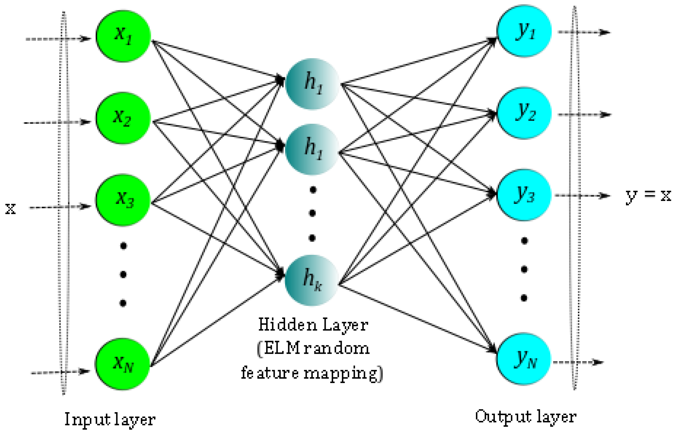
2.3. Data-Driven Sparse Basis Computation Using an ELM Autoencoder

While POD represents the energy optimal basis for a given data [56,57], they tend to be highly data-specific and do not span highly evolving flows [5]. As an alternative, one typically reconstructs data from systems with no prior knowledge using a generic basis such as Fourier functions [10,12]. Another alternative is to use radial basis function (RBFs) or Gaussian function regression to represent the data, which are known to be more robust representations of dynamically evolving flow conditions [5]. In this work, we adopt this flavor by leveraging extreme learning machines (ELMs) [19,20] which are regressors employing a Gaussian prior. An extension of this framework to learn encoding–decoding maps of a given data using an autoencoder formulation, was was proposed by Zhou et al. [21,22,23]. ELM is a single hidden layer feedforward neural network (SLFN) with randomly generated weights for the hidden nodes and bias terms followed by the application of an activation function. Finally, the output weights are computed by constraining to the output data. If we set the number of hidden nodes smaller than the dimensionality of the input data then we can get compressed feature representations of the original data as the output weight of ELM autoencoder as show in Figure 2. Given data X R N × M with N as the full state dimension and M as the number of snapshots (or simply x j R N for j = 1 , , M ), we map the full state to a K-dimensional hidden layer feature space using the ELM autoencoder as shown below in Figure 2 and Equation (13).
x j = i = 1 K ϕ i a i j = i = 1 K ϕ i h i ( x j ) = i = 1 K ϕ i g ( w i T x j + b i )
In the above equation, x j R N is the input data, j is the snapshot index, N is the dimension of input flow state, w i R N are the random input weights that map input features to the hidden layer, b i  is the random bias, g ( . ) is the activation function operating on the linearly transformed input state and ϕ i R N are the weights that map hidden layer features to the output features. Additionally, h i represents the map from input state to the ith hidden layer feature. In this autoencoder architecture, the output and input features are identical. An example of the activation function is the radial basis function as shown in Equation (14):
g ( z ) = e ( z 2 ) .
In matrix form, the linear Equation (13) can be written as in Equation (15) where a is the matrix of outputs (with elements a i j ) from the hidden layer (Equation (16)) and h ( x j ) = [ h 1 ( x j ) , , h k ( x j ) ] = [ a 1 j , , a k j ] represents the output from the K hidden nodes as a row vector for the jth input snapshot x j . h ( x j ) is also called the feature transformation that maps the data, x j from the N dimensional input space to the K dimensional hidden layer feature space a .
X = Φ a
a = a 1 1 a k 1 a 1 M a k M ) T = h ( x 1 ) h ( x M ) T = h 1 ( x 1 ) h k ( x 1 ) h 1 ( x M ) h k ( x M ) T .
The output weights can be written in matrix form as in Equation (17) and X as in Equation (18).
Φ = ϕ 1 1 ϕ 1 N ϕ k 1 ϕ k N T
X = x 1 1 x N 1 x 1 M x N M T .
Using Equation (15), Φ can be solved as in Equation (19) using the Moore–Penrose pseudo-inverse.
Φ t r a i n = Φ = X a + = X a t r a i n + .
The primary difference between POD and the ELM autoencoder is that in the former, the basis Φ is learned first whereas in ELM, the features a are derived first followed by Φ . The other major difference is that the columns of the POD basis vectors represent coherent structures contained in the data snapshots, whereas the interpretation of the ELM basis is not clear.

2.4. Measurement Locations, Data Basis, and Incoherence

Recal from Section 2.1, that the reconstruction performance is strongly tied to the measurement matrix C being necessarily incoherent with respect to the low-dimensional basis Φ [12], which is usually accomplished by employing a random sampling for the sensor placement. In practice, one can adopt two types of random sampling of the data, namely, single-pixel measurements [7,35,58] or random projections [10,12,42]. Typically, single-pixel measurements refers to measuring information at the particular spatial locations, such as measurements by unmanned aerial systems (UAS) in the atmospheric fields. Another popular choice of sensing method in the compressive sensing or image processing community is random projections, where the measurement matrix is populated using normally distributed random numbers on to which the full state data is projected. In theory, the random matrix is highly likely to be incoherent with any fixed basis [12], and hence efficient for sparse recovery purposes. However, for most of the fluid flow applications, the sparse data is usually sourced from point measurements and hence, the single-pixel approach is practically relevant. Irrespective of the approach adopted, the measurement matrix C (Equations (1) and (2)) and basis Φ should be incoherent to ensure optimal sparse reconstruction. This essentially implies that one should have sufficient measurements distributed in space to excite the different modes relevant to the data being reconstructed. Mathematically, this implies that C Φ is full rank and invertible.
There exist metrics to estimate the extent of coherency between C and Φ in the form of a coherency number, μ as shown in Equation (20) [59]:
μ ( C , Φ ) = N · max i P , j K c i , ϕ j ,
where c i is a row vector in C and ϕ j is a column vector of Φ . μ typically ranges from 1 (incoherent) to N (coherent). The smaller the μ , the less measurements one needs to reconstruct the data in an l 1 sense. This is because the coherency parameter enters as the prefactor in the lower-bound for the sensor quantity in l 1 -based CS for accurate recovery. There exist optimal sensor placement algorithms such as K-means clustering, the data-driven online sparse Gaussian processes [60], physics-based approaches [61], and mathematical approaches [15] that minimize the condition number of Θ and maximize the determinant of the Fisher information matrix [62]. A thorough study on the role of sensor placement on reconstruction quality is much needed and an active topic of research, but not considered within the scope of this work. For this analysis, which focuses on the role of basis choice on sparse reconstruction, we simplify the sensor placement strategy by using the Matlab function randperm (N) to generate a random permutation from 1 to N and the first p values are chosen as the sampling locations in the data. However, to minimize the impact of sensor placement on the conclusions of this study, we perform an ensemble of numerical experiments with different random sensor placements and explore averaged error metrics to make our interpretations robust. Further, in most practical flow measurements the sensor placement is random or based on knowledge of the flow physics. The current approach can be considered to be consistent with that strategy.

2.5. Sparse Recovery Framework

The algorithm used in this work is inspired from the gappy POD or GPOD framework [25] and can be viewed as an l 2 minimization reconstruction of the sparse recovery problem, summarized by Equations (4)–(6) with Φ composed of K M basis vectors, i.e., the dimension of a is K M . At this point, we remind the reader of naming conventions adopted in this paper: the instantaneous jth full flow state is denoted by x j R N , whereas the entire set consisting of M snapshots is assembled into a matrix form denoted by X R N × M . In the following, we focus on single snapshot reconstruction and the extension to multiple snapshots is trivial, i.e., each snapshot can be reconstructed sequentially or in some cases be grouped together as a batch reconstruction. This allows for such algorithms to be easily parallelized.
The primary difference between the SR framework in Equation (4) as used by the image processing community and GPOD [14,15,25,57] as shown in Equation (22) is the construction of the measurement matrix C and the sparse measurement vector x ˜ j . For the purposes of this discussion, we will consider reconstruction of a single snapshot. In SR (Equation (4)) x ˜ j R P is a compressed version containing only the measured data, whereas in the GPOD framework, x ˜ j R N is a masked version of the full state vector, i.e., values outside of the P measured locations are zeroed out to generate a filtered version of x j . For high resolution data x j R N with the chosen basis ϕ k R N , the low-dimensional features, a j R K are obtained from the relationship shown below:
x j = k = 1 K ϕ k a k j .
The masked (incomplete) data x ˜ j R N , corresponding measurement matrix C, and mask vector m R N are related by:
x ˜ j = < m · x j > = C x j ,
where C R N × N . Therefore, the GPOD algorithm results in a larger measurement matrix with numerous rows of zeros as shown in Figure 3 (compare with Figure 1). To bypass the complexity of handling the N × N matrix, a mask vector, m N × 1 with 1 s and 0 s operates on x j through a point-wise multiplication operator < · > . As an illustration, the point-wise multiplication is represented as x ˜ j = < m j · x j > for each snapshot j = 1 M where each element of x j multiplies the corresponding element of m j . This is applicable when each data snapshot x j has its own measurement mask m j , which is a useful way to represent the evolution of sparse sensor locations over time. The SR formulation in Equation (4) can also support time varying sensor placement, but would require a compression matrix C i that changes with each snapshot. This approach is by design much more computationally and storage intensive, but can handle situations that do not incorporate point sensor compression.
The goal of the SR procedure is to recover the full data from the masked data given in Equation (23) by approximating the coefficients a ¯ j (in the l 2 sense) with basis ϕ K , learned offline using training data (snapshots of the full field data).
x ˜ j m k = 1 K a ¯ k j ϕ k .
The coefficient vector a ¯ j cannot be computed by direct projection of x ˜ j onto Φ as these are not designed to optimally represent the sparse data. Instead, one needs to obtain the “best” approximation of the coefficient a ¯ j , by minimizing the error E j in the l 2 sense as show in Equation (24).
E j = x ˜ j m k = 1 K a ¯ k j ϕ k 2 2 = x ˜ j m · Φ a ¯ j 2 2 = x ˜ j C Φ a ¯ j 2 2 .
In Equation (24) we see that m acts on each column of Φ through a point-wise multiplication operation, which is equivalent to masking each basis vector ϕ k . Unless the sensor placement is constant with time, we remind one that the above formulation is valid for a single snapshot reconstruction where the mask vector, m j , changes with every snapshot x ˜ j for j = 1 , , M . Thus, the error E i represents the single snapshot reconstruction error that will be minimized to compute the approximate features a ¯ j . It can easily be seen from below that one will have to minimize the different E j ’s sequentially to learn the entire coefficient matrix, a ¯ R K × M for all M snapshots. Denoting the masked basis functions as ϕ k ˜ ( z ) = < m ( z ) · ϕ k ( z ) > , Equation (24) is rewritten as in Equation (25).
E j = x ˜ j k = 1 K a ¯ k j ϕ ˜ k 2 2 .
In the above formulation, Φ ˜ is analogous to C Φ = Θ in Equation (4). To minimize E j , one computes the derivative with respect to a ¯ j and equates it to zero as below:
a ¯ j ( E j ) = 0 .
The result is the linear normal equation given by Equation (27):
M a ¯ j = f j ,
where M k 1 , k 2 = ϕ ˜ k 1 , ϕ ˜ k 2 or M = Φ ˜ T Φ ˜ and f k j = x ˜ j , ϕ ˜ k or f j = Φ ˜ T x ˜ j . The reconstructed solution is given by Equation (28) below:
x ¯ j = k = 1 K ϕ k a ¯ k j .
Algorithm 1 summarizes the above SR framework assuming the basis functions ( ϕ k ) are known. The above solution procedure for sparse recovery is the same as that described in Section 2.1 except for the dimensions of x ˜ and C.
Algorithm 1: l 2 -based algorithm: Sparse reconstruction with known basis, Φ .
Fluids 03 00088 i001

2.6. Algorithmic Complexity

The cost of computing both the ELM and POD basis is O ( N × M 2 ) where N is the full reconstructed flow state dimension and M is the number of snapshots. The cost of sparse reconstruction turns out to be O ( N × K × M ) for both the methods, where K M is the system dimension chosen for reconstruction. Naturally, for many practical problems with an underlying low-dimensional structure, POD is expected to result in a smaller K than ELM. This will reduce the sensor quantity requirement and the reconstruction cost to a certain extent. Further, since the number of snapshots (M) is also tied to the desired basis dimension (K), a larger K requires a larger M and in turn a higher cost to generate the basis.

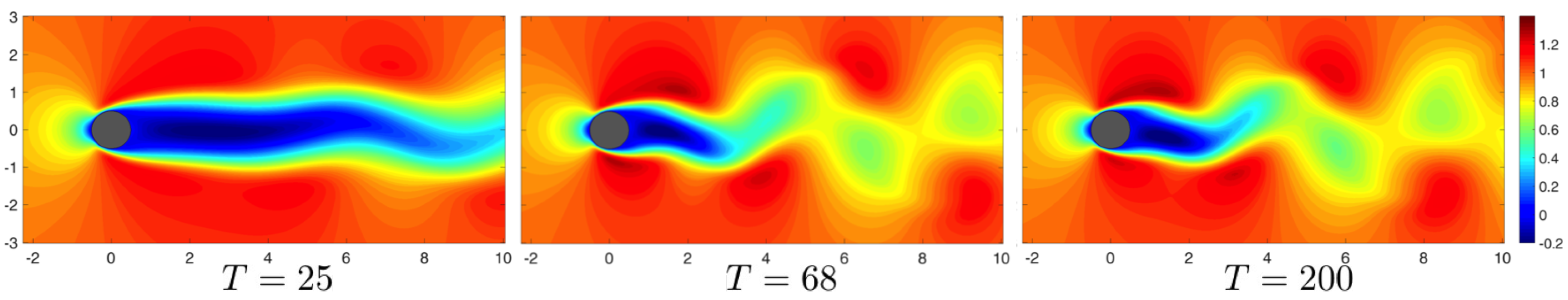
3. Data Generation for Canonical Cylinder Wake

Studies of cylinder wakes [33,63,64,65] have attracted considerable interest from the data-driven modeling community for their particularly rich flow physics content, encompassing many complexities of nonlinear fluid flow dynamical systems and ease of simulation using established computational fluid dynamics (CFD) tools. In this study, we explore data-driven sparse reconstruction for the cylinder wake flow at R e = 100 . It is well known that the cylinder wake is initially stable and then becomes unstable before settling into a limit-cycle attractor. To illustrate this dynamics, snapshots showing evolution of the stream-wise velocity component (u) are shown in Figure 4, for R e = 100 .
For this study, we focus on reconstruction in the temporal regime with periodic limit cycle dynamics, in contrast to our earlier work [35] where we focused on reconstruction in both the limit cycle and transient regimes. The two-dimensional cylinder flow data is generated using a spectral Galerkin method [66] to solve incompressible Naiver–Stokes equations, as shown in Equations (29)–(31) below:
u x + u y = 0 ,
u t + u u x + v u y = P x + ν 2 u ,
v t + u v x + v v y = P y + ν 2 v ,
where u and v are the horizontal and vertical velocity components, P is the pressure field, and ν is the fluid viscosity. The rectangular domain used for this flow simulation is 25 D < x < 45 D and 20 D < y < 20 D , where D is the diameter of the cylinder. For the purposes of this study, data from a reduced domain, i.e., 2 D < x < 10 D and 3 D < y < 3 D , is used. The mesh was designed to sufficiently resolve the thin shear layers near the surface of the cylinder and transit wake physics downstream. For the case with R e = 100 , the grid includes 24,000 points. The computational method employed is a fourth order spectral expansion within each element in each direction. The sampling rate for each snapshot output is chosen as Δ t = 0.2 s.
While the use of the 2D version of the incompressible Navier–Stokes equations, to compute the full cylinder data is justified for laminar flows, for turbulent flows this full flow state will be a high resolution 3D dataset with large state dimension that can escalate the computational complexity. The increased state dimension can severely impact the cost of POD-Galerkin based reduced order models (ROMs) through the nonlinear term, whose computation scales with the large full state dimension. This, in turn, can negate the advantages of such ROMs for large-scale systems. To accelerate such models, methods such as gappy POD [14,15,25], the discrete empirical interpolation method (DEIM) [67] and missing point estimation (MPE) [68], estimate a low rank mask matrix to approximate the full state nonlinear term using data at sparse sampled locations. This allows for the expensive inner products using high-dimensional vectors to be replaced with low-dimensional ones. Given the strong connections between compressive sensing, sparse reconstruction, and gappy POD, it is not far fetched to adopt the algorithms presented in this work for complexity reduction of POD-Galerkin models. Dimitriu et al. [69] compares the performance of these hyper reduction techniques for use in online model computations and observes that DEIM and GPOD generate similar sensor placement, online computational cost, and accuracy. On the other hand, MPE was less computationally expensive in the offline cost, but prone to inaccuracies.

4. Sparse Reconstruction of Cylinder Wake Limit-Cycle Dynamics

In this section, we explore sparse reconstruction of fluid flows at R e = 100 using the above SR infrastructure for the cylinder flow with well-developed periodic vortex shedding behavior. The GPOD formulation is chosen over the traditional SR formulation to bypass the need for maintaining a separate measurement matrix, since we are focusing only on point sensors in this discussion. Maintaining a separate measurement matrix involves storing a lot of elements that are zeros which do not impact the matrix multiplications in both the versions of the SR algorithm. In most cases reported here, Tikhonov regularization is employed to reduce overfitting and provide uniqueness to the solution. In this study, we choose 300 snapshots of data corresponding to a non-dimensional time ( T = U t D ) of T = 60 with a uniform temporal spacing of d T = 0.2 s. T = 60 corresponds to multiple (≈10) cycles of periodic vortex shedding behavior for flow with R e = 100 , as seen from the temporal evolution of the POD coefficients as shown in Figure 5 below.

4.1. Sparse Reconstruction Experiments and Analysis

For this a priori assessment of SR performance, we reconstruct sparse data from simulations where the full field representation is available. The sparse sensor locations are chosen as single point measurements using a random sampling of the full field data and these locations are fixed for the ensemble of snapshots used for the reconstruction. Specifically, we employ the Matlab function randperm (N) to generate random permutation from 1 to N with the first p values chosen as the sensor locations. Reconstruction performance is evaluated by comparing the original simulation predicted field with those from SR using both POD and ELM basis, across the entire ensemble of numerical experiments. We undertake this approach in order to assess the relative roles of system sparsity (K), sensor sparsity (P), and sensor placement (C) for both the POD and ELM-based SR. In particular, we aim to accomplish the following through this study: (i) check if P > K is a necessary condition for accurate reconstruction of the fluid flow irrespective of the basis employed; (ii) determine the dependence of the estimated sparsity metric K for the desired reconstruction quality on the choice of basis; and (iii) understand how sensor placement impacts reconstruction quality for different choice of basis.
To learn the data-driven basis, we employ the method of snapshots [55] as shown in Equations (9)–(12) for POD and train an autoencoder as shown in Equations (13)–(19) for the ELM basis. For the numerical experiments described here, the data-driven basis and coefficients are obtained from the full data ensemble, i.e., M = 300 snapshots corresponding to T = 60 non-dimensional times. This gives rise to at most M basis for use in the reconstruction process in Equation (3), i.e., a candidate basis dimension of N b = M . While this is obvious for the POD case, we observe that for ELM K M does not improve the representational accuracy (see Figure 6). As shown in Table 1, the choice of algorithms depend on the choice of system sparsity (K), data sparsity (P), and the dimension of the candidate basis space, N b . Recalling from the earlier discussion in Section 2, we see that P K would require an l 2 method for a desired reconstruction sparsity K as long as P N b . In the case of POD, the basis are energy optimal for the training data and hence, contain built-in sparsity. That is, as long as the basis is relevant for the flow to be reconstructed, retaining only the most energetic modes (basis) should generate the best possible reconstruction for the given sensor locations. Therefore, the POD basis needs to be generated once and the sparsity level of the representation is determined by just choosing to retain the first few modes in the sequence. On the other hand, ELM basis does not have a built-in mechanism for order reduction. The underlying basis hierarchy for the given sparse data is not known a priori and therefore requires one to search for the K most significant bases among the maximum possible dimension of N b = M , using sparsity promoting l 1 methods. However, for this work we bypass the need for the l 1 algorithm in favor of the less expensive l 2 method by learning a new set of basis for each choice of K = N b < M . The increased cost of l 1 methods such as the iterative thresholding algorithms [28,70] require multiple solutions of the least-squares problem before a sparse solution is realized.

4.2. Sparsity and Energy Metrics

For this SR study, we explore the conditions for accurate recovery of information in terms of data sparsity (P) and system sparsity (K), which also represents the dimensionality of the system in a given basis space. In other words, sparsity represents the size of a given basis space needed to capture a desired amount of energy. As long as the measurements are incoherent with respect to the basis Φ and the system is overdetermined, i.e., P > K , one should be able to invert Θ to recover the higher dimensional state, X. From earlier discussions in Section 2, we know P > K is a sufficient condition for accurate reconstruction using l 0 minimization. Thus, both interpretations require a minimum quantity of sensor data for accurate reconstruction, which is verified through numerical experiments in Section 4.3.
In this section, we describe how the different system sparsity metrics, K = N b , are chosen for the numerical experiments with both POD and ELM basis. Since the basis spaces are different, a good way to compare the system dimension is through the energy captured by the respective basis representations. For POD one easily defines a cumulative energy fraction captured by the K most energetic modes, E K , using the corresponding singular values of the data as shown in Equation (32).
E K = k = 1 K λ k ( λ 1 + λ 2 + + λ M ) × 100 ,
In the above, the singular values λ are computed from Equation (10), and M is the total number of possible eigenvalues for M snapshots.
For the cylinder flow case with R e = 100 , one requires two and five POD modes to capture 95 % and 99 % of the energy content, respectively, indicative of the sparsity of the dynamics in this basis space. In this case, we compute e r r K P O D = X Φ 1 K P O D a 1 K P O D 2 , where Φ 1 K P O D a n d a 1 K P O D represent the matrix comprising of the K POD bases and the corresponding coefficients for the different snapshots, respectively. The approach of tying the system sparsity with the energy content or alternatively the error obtained by reconstructing the basis with full data, allows one to compare different choices of basis space. Since there exists no natural hierarchy for the ELM basis, we characterize the system sparsity K through the reconstruction error (with respect to the true data) obtained during the training of the ELM network as in Equation (19). This is computed as the 2-norm of the difference between the ELM trained flow field, i.e., the ELM output layer, X t r a i n , K E L M = Φ t r a i n , K E L M a t r a i n , K E L M and the exact flow field, i.e., the ELM input layer, X e x a c t . Mathematically, we compute e r r K E L M = X X t r a i n , K E L M 2 . To relate the system dimensionality in the ELM and POD spaces and assess their relative sparsity, we compare the energy captured for different values of K in terms of their respective reconstruction errors as shown in Figure 6. We note that the ELM training in Equation (13) employs random weights which produces variability in the error metric, e r r K E L M . To minimize this variability, we perform a set of twenty different training for each value of K E L M and compute the average error as plotted in Figure 6.
From this, we observe that for ELM, K = 99 produces the same representation error as produced by using just K = 2 for the POD basis. It turns out that K = 2 for POD captures 95 % of the energy as per Equation (32), i.e., K 95 E L M = 99 and K 95 P O D = 2 . The decay of e r r K E L M with K is nearly exponential, but slower than that observed for e r r K P O D . Further, for K M , the ELM training over-fits the data which drives the reconstruction error to near zero. To assess SR performance across different flow regimes (that have different K 95 ) with different values of K we define a normalized system sparsity metric, K = K / K 95 and a normalized sensor sparsity metric, P = P / K 95 . This allows us to design an ensemble of numerical experiments in the discretized P K space and the outcomes can be generalized. In this study, the design space is populated over the range 1 < K < 6 and 1 < P < 12 for POD SR, and for ELM SR the range is 1 < K < 3 and 1 < P < 6 as the K is bounded by the total number of snapshots, M = 300 . The lower bound of one is chosen such that the minimally accurate reconstruction captures 95 % of the energy. If one desires a different reconstruction norm, then K 95 can be changed to K x x without loss of generality and the corresponding K-space modified accordingly. Alternately, one can choose E K , the normalized energy fraction metric to represent the desired energy capture as a fraction of E K 95 , but this is not used in this study.
To quantify the l 2 reconstruction performance, we define the mean squared reconstruction error as shown in Equation (33) below:
ϵ K , P S R = 1 M 1 N j = 1 M i = 1 N ( X i , j X ¯ i , j S R ) 2 ,
where X is the true data, and X ¯ S R is the reconstructed field using sparse measurements as per Algorithm 1 and either POD or ELM as the choice of basis. N and M represent the state and snapshot dimensions affiliated with indices i and j, respectively. Similarly, the mean squared error ϵ K 95 F R and ϵ K F R for the full reconstruction from both POD and ELM based SR are computed as:
ϵ K 95 F R = 1 M 1 N j = 1 M i = 1 N ( X i , j X ¯ i , j F R , K 95 ) 2 ,
ϵ K F R = 1 M 1 N j = 1 M i = 1 N ( X i , j X ¯ i , j F R , K ) 2 ,
where X ¯ F R is the full field reconstruction using exactly computed coefficients for both POD and ELM cases. K 95 = K 95 / K 95 = 1 is the normalized system sparsity metric (i.e., number of basis normalized by K 95 ) corresponding to 95 % energy capture and K = K / K 95 represents the desired system sparsity. The superscript F R corresponds to the full reconstruction using exactly computed coefficients a. For POD, this is simply a = Φ T X as per Equation (12). However for ELM, a = Φ + X where Φ = Φ t r a i n and is obtained as per Equation (19). However, this computed a is not the same as a t r a i n used in the ELM training step (Equation (19)) as Φ + Φ is not exactly an identity matrix. Therefore, the error in the pseudo-inverse computation of Φ produces two sets of a, one from direct estimation using the ELM basis ( a = Φ + X ) and the other from ELM training step ( a t r a i n ) through a direct estimation. This results in two types of error estimations with a t r a i n being used to estimate e r r K E L M and a being used to compute ϵ K 95 F R in Equation (34) and ϵ K F R in Equation (35).
Using the above definitions, we can now generate normalized versions of the absolute ( ϵ 1 ) and relative ( ϵ 2 ) errors as shown in Equation (36). ϵ 1 represents the SR error normalized by the corresponding full reconstruction error for 95 % energy capture. ϵ 2 represents the normalized error relative to the desired reconstruction accuracy for the chosen system sparsity, K. These two error metrics are chosen so as to achieve the twin goals of assessing the overall absolute quality of the SR in a normalized sense ( ϵ 1 ) and the best possible reconstruction accuracy for the chosen problem set-up (i.e., P , K ). Thus, if the best possible reconstruction for a given K is realized then ϵ 2 will take the same value across different K . This error metric is used to assess relative dependence of P on K for the chosen flow field. On the other hand, ϵ 1 provides an absolute estimate of the reconstruction accuracy so that minimal values of P   and   K needed to achieve a desired accuracy can be identified.
ϵ 1 = ϵ K , P S R ϵ K 95 F R , ϵ 2 = ϵ K , P S R ϵ K F R .

4.3. Sparse Reconstruction of Limit-Cycle Dynamics in Cylinder Wakes Using the POD Basis

As the first part of this study is designed to establish a baseline SR performance using the POD basis similar to that performed in Reference [35], we carried out a series of POD-based sparse reconstruction (SR) experiments corresponding to different points in the P K design space and spread over the different sensor placements. In these experiments, the sparse data is obtained from a priori high resolution flow field data with randomly placed sparse sensors that do not change with each snapshot. The randomized sensor placement in this case is controlled using a seed value in Matlab which is fixed for all the experiments within a given design space. By computing the errors as described in Section 4.2 across the K P space, the contours of ϵ 1 and ϵ 2 at R e = 100 for a few different random sensor placements are shown in Figure 7 and Figure 8.
The relative error metric ϵ 2 (the right column in Figure 7 and Figure 8), shows that the smaller errors (both light and dark blue regions) are predominantly located over the region where P > K , separated from the other region using a diagonal line corresponding to P = K . This indicates that the over specified SR problem with P > K , i.e., having more sensors than the dimensionality chosen to represent the system yields good results in terms of ϵ 2 . For small P , the normalized relative error can reach as high as O ( 10 1 10 2 ) . Since ϵ 2 is normalized by the error contained in the exact K-sparse POD reconstruction, this metric represents how effectively the sparse sensor data can approximate the K-sparse solution using l 2 minimization. In principle, the exact K-sparse POD reconstruction is the best possible outcome to expect irrespective of how much sensor data is available, as long as K = N b . We note that by constraining the SR problem by choosing the desired energy sparsity K, the l 2 reconstruction is reconciled with the l 0 minimization solution [35]. Consistent with the observations in Reference [35], we observe that ϵ 1 contours adhere to an L-shaped structure indicating that absolute normalized error reduces as K is increased to capture more energy contained in the full field data.
While this ‘best’ reconstruction is almost always observed for the higher values of P and K for the different sensor placements, there appear to be some exceptions. Notably, for a few sensor placement choices (seed 101 in Figure 7 and 108 in Figure 8), a small portion of ϵ 1 in the region abutting the P = K line shows nearly an order of magnitude higher error, O ( 10 1 ) (colored as red in Figure 7 and Figure 8) as compared to the expected values of O ( 1 ) observed for sensor placement using seeds 102 and 109 in Figure 7 and Figure 8, respectively.
We probe these ‘anomalous’ points by visualizing the SR of a random snapshot along with their corresponding sensor placements to deduce possible insight into the reason for high errors in terms of sensor placement. In Reference [35], it was shown that although the coherency number μ was small for a given sensor placement choice, the sparse data points should still span the physics to be captured. Inspired by this, we experiment the impact of sensor placement for two regions corresponding to P K and P > K .
At point 1 (where P = K ) for sensor placement with seed 101 (Figure 7) both ϵ 1 and ϵ 2 indicate an order of magnitude higher error relative to its neighborhood. But for the same point with modified sensor placement using seed 102, we observe nearly an order of magnitude lower error. Comparing the SR flow fields for both the sensor placements with different seeds, as shown in Figure 9, we see that seed 102 places more data points in the wake of the cylinder as compared to that for seed 101, hence the better reconstruction. A follow up study is needed to explore data-driven methods for optimal sensor placement and their influence on SR error. Mathematically, data points in the cylinder wake region excite the most energetic POD modes as compared to sensors placed elsewhere. This is clearly shown in Reference [35] where the coefficients or features corresponding to the most energetic POD modes are erroneous when recovered using inadequate sensor placement. This trend is observed even for the under specified (ill-posed) case with P < K , i.e., point 3 in Figure 8 for cases with different sensor placement (seeds 108 and 109) as shown in Figure 9. As part of the Appendix, we further illustrate the mechanism of how sensor placement impacts the predictions in Figure A1 where we compute the reconstructed POD features corresponding to P = 3 and K = 3 for the four different sensor placement cases (seeds 101–102 and 108–109) discussed here. This plot clearly shows that for the cases with inadequate sensor placement (seed 101 & 108), we observe large deviations of the predicted POD features for those corresponding to full data reconstruction. Not surprisingly, the SR cases with adequate sensor placement show closer agreement with the exact POD features obtained by projecting the full data onto the POD basis space.
In conclusion, we observe that although the POD-based SR is very efficient in terms of sensor quantity requirement, the reconstruction errors are sensitive to sensor location even when P K . For cases with P > K (points 2 and 4 in Figure 7 and Figure 8), we observe that this sensitivity to sensor placement is highly minimized although small differences exist as shown in Figure 10. This is because, an increase in the number of measurement points enhances the probability of locating points within the cylinder wake.
In order to generalize the error metrics computed in Figure 7 and Figure 8, we perform an ensemble of ten different sensor placements corresponding to seeds ranging from 101 to 110. We plot the error contours corresponding to maximum and minimum errors estimated across the entire P K design space and also the average error over this ensemble, as shown in Figure 11. The maximum error is found for seed 108 and minimum error for seed 109. The average error contours represent the most probable SR outcome independent of the anomalies from sensor placement.

4.4. Sparse Reconstruction Using the ELM Basis

The previous section focused on the SR performance of limit-cycle cylinder wake dynamics using the POD basis; which was shown to perform well if certain conditions are met, namely, P > K and reasonable sensor placement. A key issue identified with POD-based SR for low-dimensional systems, such as the cylinder wake dynamics, is that it requires a small number of sensors for reconstruction, but is sensitive to their placement. As observed in Section 4.2, ELM requires a greater number of basis for the same amount of energy capture. For example, for 95 % energy capture, we will need K = 99 for ELM and just K = 2 for POD. While SR using ELM basis is similar in concept, the non-orthogonality of the ELM basis and their relative lack of sparsity brings about certain differences. It was shown in Section 4.2 that there exist two different kinds of errors—a training error and the reconstruction error. If the ELM basis were to be orthogonal just like the POD basis, both these errors (and the ELM features a and a t r a i n ) will be equivalent. Second, in Section 2.3 the algorithm for computing the basis using an ELM autoencoder uses randomly chosen input weights when generating the K-dimensional hidden layer features, which represents the low-dimensional representation. Consequently, the realized ELM basis are not unique, unlike the POD basis for a given training data set. It was observed from our numerical experiments that while the sensitivity of this randomness in the ELM basis to the reconstruction errors is not severe, it is perceptible. To analyze the performance of ELM-based SR, we carry out two different types of analysis. The first explores of the effect of randomness in the weights used within ELM training, while fixing the sensor placement. The second explores randomness from the choice of sensor placement for a given ELM basis.
To accomplish the first, we compute the normalized ELM-based SR error metrics ϵ 1 and ϵ 2 using ten different choices for the random input weight sets. The contours corresponding to the seed with maximum, minimum, and the average error are shown in Figure 12. These plots clearly show that there exist very little sensitivity to the choice of random weights in the ELM training. Further, as was the case for the POD-based SR, the region of good reconstruction is separated from the high-error region by the straight line corresponding to P = K indicating that similar normalized performance bounds exist for both POD (orthogonal basis) and ELM (non-orthogonal basis).
The second part of the ELM-based SR analysis is to assess the effect of sensor placement on the reconstruction performance for a fixed choice of random weights in the ELM training. To accomplish this, we consider an ensemble of numerical simulations with ten different choices of sensor placement across the entire P K design space. Figure 13 shows the normalized error contours for the case with sensor placement resulting in the maximum error, minimum error, and the average error field over the entire ensemble. Once again, we observe accurate SR performance for P > K , which results in a well-posed reconstruction problem. Further, we observe that the choice of sensor placement has very minimal impact on the overall SR error metrics. This is not surprising given that ELM requires more sensors as compared to POD to achieve the same level of reconstruction accuracy. As verification, we have included in Appendix A, Figure A2 and Figure A3 that compare the reconstruction of a single snapshot flow field and the corresponding ELM features respectively for two different sensor placement choices. The two sensor placements correspond to cases with maximum and minimum errors observed in Figure 13 at design points using K = 2 and P = 3 . The comparison of the reconstructed snapshots using sparse and full data shown in Figure A2 do not show any significant errors (in comparison to the full data representation) upon visual inspection. However, comparison of the SR predicted ELM features with those for the FR display strong sensitivity to sensor placement. In particular, we observe that for sensor placement with seed 101, the ELM features are grossly incorrect as compared to that for seed 106. In spite of this, the visually accurate prediction of the reconstructed field for seed 101 is surprising and can be explained as follows. In the ELM-based SR with random sensor placement, a significant number of these sensors find themselves in the most dynamically relevant regions of the flow and even if a few of the sensors were to be misplaced, the contribution to the overall error metric from this is much smaller as compared to POD-based SR. The second speculation is that the higher dimensional ELM basis represents redundant structures that enable it to be relatively insensitive to non-optimal sensor placement. This suggests that the ELM basis space could be represented more compactly, possibly through orthogonalization for improved performance, which will be explored in the future.

5. Conclusions

In this article, we explore the interplay of sensor quantity (P) and placement, and system dimensionality or sparsity (K) using optimal data-driven POD & ELM bases with an l 2 sparse reconstruction (SR) of a cylinder wake flow. Particularly, we attempted to (i) explore whether the relationship between system dimensionality and sensor quantity for accurate reconstruction of the fluid flow is independent of the basis employed, and (ii) understand the relative influence of sensor placement on the different choices of SR basis.
Regarding the first goal of this study, we observed that the choice of the sparse basis plays a crucial role in the SR performance as it determines system dimensionality or sparsity (K) and in turn the sensor quantity (P) to ensure the problem is well posed. Specifically, in terms of non-dimensional variables ( P , K ) normalized using the characteristic system dimension for a given basis ( K 95 corresponding to 95 % energy ), all one needed was the system to be well posed, i.e., P > K to realize reasonably accurate reconstruction. This requirement turned out to be independent of the chosen basis. However, the POD/SVD basis represent optimal energy capture for a given training data and allows for efficient energy-based SR. Further, unlike generic basis spaces such as Fourier or radial basis functions, the data-driven POD basis needs to be highly flow relevant as it retains the K most energetic modes for reconstruction and implicitly generates the K-sparse solution for the given sensor locations. For the more generic ELM basis, relevance to the reconstructed flow is less important, but there exists no inherent hierarchy in the basis vectors. Thus, when using a smaller number of sensors, one may need to employ the l 1 regularized least squares algorithms to generate meaningful results. In addition, training the ELM network with partially random weights generates a new K-dimensional basis space every time. As such ELM basis are not designed to optimally capture the variance of the data, they are less parsimonious and non-orthogonal when compared to the orthogonal POD basis. For the datasets considered in this this study, one needed an order of magnitude larger number of ELM basis and sensors as compared to POD modes to realize the same reconstruction accuracy.
As for the second goal of this study, we observed that the ELM-based SR was less sensitive to the choice of random sensor placement as compared to the POD-based SR. With the POD basis being low-dimensional, the SR problem required very few sensors for accurate reconstruction of this cylinder wake dynamics, but displayed sensitivity to the choice of random sensor placement. To account for this sensitivity, all the error metrics reported in this article were ensemble averaged over multiple choices of sensor placement. On the other hand, ELM-basis being relatively high dimensional required substantially more sensors for accurate reconstruction and turned out to be less sensitive to the choice of random sensor placement. To illustrate this, we showed the variability between the worst and best reconstructions across the different choices of sensor locations is insignificant and not discernable by the naked eye. Therefore, we expect optimal sensor placement algorithms to offer more value in POD-based SR than in ELM-based SR. On a related note, we have provided a brief overview of different classes of methods for estimating optimal sensor locations in Section 2.4, which operate on modifying the structure of the matrix Θ . Therefore, these algorithms should be equally applicable to both POD and ELM-based frameworks.

Author Contributions

B.J. conceptualized the research with input from A.A.-M. and C.L. A.A.-M. and C.L. developed the sparse reconstruction codes with input from B.J. B.J. and A.A.-M. analyzed the data. A.A.-M. and C.L. developed the first draft of the manuscript and B.J. edited the final written manuscript.

Funding

This research was supported by Oklahoma State University start-up grant and also through a Cooperative Research Agreement (CRA) with Baker Hughes General Electric, Oklahoma City, OK.

Acknowledgments

We acknowledge computational resources from Oklahoma State University High Performance Computing Center (HPCC). We also thank the anonymous reviewers for their detailed and thought-provoking comments that helped us improve the manuscript.

Conflicts of Interest

The authors declare no conflict of interest.

Appendix A. Comparison of Predicted ELM Features and Snapshot Reconstruction

Figure A1. Sparse reconstructed (SR) POD coefficients for different sensor placements compared with full reconstruction (FR) for a given K = 3 .
Fluids 03 00088 g0a1
Figure A2. Comparison of ELM-based parse reconstruction with full reconstruction flow fields for a single snapshot at T = 48.8, using random sensor placement with seed = 101 (maximum reconstruction error) and seed = 106 (minimum reconstruction error) from the choice of ten different experiments. Blue solid line: FR. Red dashed line: SR. Black stars: sensor locations. (a) Seed = 101 (max error); and (b) Seed = 106 (min error).
Fluids 03 00088 g0a2
Figure A3. Comparison of the sparse reconstructed (SR) ELM features with the corresponding full data reconstruction (FR) predicted features. The two SR cases correspond to sensor placement with maximum error (seed = 101) and minimum error (seed = 106).
Fluids 03 00088 g0a3

Appendix B. Impact of Retaining the Data Mean for Sparse Reconstruction

The SR framework described through the early sections of this article removed the mean before computing the data-driven basis as a matter of choice. As mentioned in Section 2.2, this step is not critical to the success of this method. In this section, we compare the effect of retaining the mean, against removing it, on the computed basis and the reconstruction performance. Figure A4 compares the first five POD modes using data with and without the mean. It is observed that retaining the mean (i.e., just the SVD step) generates an extra ‘mean’ POD mode that carries significant energy but the rest of the basis is similar to those computed after removing the mean. This choice in essence shifts the resulting energy spectrum. Figure A5 compares the normalized mean squared POD-based SR errors. This comparison clearly shows that both the variants of the SR framework yield nearly similar error distribution over the P K space for the most part. However, the SR with the mean retained have slightly increased errors in the region P K .
Figure A4. Isocontours of first five POD modes with and without removing the mean from the snapshot data for cylinder wake flow with R e = 100. (a) 1st POD mode (with mean); (b) 1st POD mode (without mean); (c) 2nd POD mode (with mean); (d) 2nd POD mode (without mean); (e) 3rd POD mode (with mean); (f) 3rd POD mode (without mean); (g) 4th POD mode (with mean); (h) 4th POD mode (without mean); (i) 5th POD mode (with mean); and (j) 5th POD mode (without mean).
Fluids 03 00088 g0a4aFluids 03 00088 g0a4b
Figure A5. The isocontours of the normalized mean squared POD-based sparse reconstruction errors ( l 2 norms). The top figures correspond to the case with mean removed for learning the basis. The bottom figures correspond to the case with the mean retained. Left: normalized absolute error metric, ϵ 1 . Right: normalized relative error metric, ϵ 2 . (a) ϵ 1 (without mean); (b) ϵ 2 (without mean); (c) ϵ 1 (with mean); and (d) ϵ 2 (with mean).
Fluids 03 00088 g0a5aFluids 03 00088 g0a5b

Appendix C. POD-Based Sparse Reconstruction for Cylinder Wake with Re = 800

In order to assess the SR performance for high Reynolds number flows, we use wake data at R e = 800 . The data generation for this simulation required higher grid resolution to resolve the thinner boundary layers on the cylinder surface. As one would expect, the system dimension also increases with Reynolds number which in turn requires more sensors for reconstruction. The focus of this study is to understand how normalized reconstruction errors depend on normalized system dimension and sensor quantity for different choice of bases. In this appendix, we reproduce similar analysis of Section 4.3 and Section 4.4 for a higher dimensional system. Figure A6 shows the normalized error metrics for POD-based SR using different choices of sensor locations corresponding to the maximum, minimum, and the average accuracy expected for this random sensor placement framework. While the overall distribution of the error metrics are similar to the lower-dimensional case, we observe that the high accuracy region for ϵ 2 is determined by P 2 K for this high-dimensional case (in contrast to and P K for the low-dimensional case). The role of sensor placement on this observation is expected, but requires further investigation. ELM-based SR for this higher-dimensional system mimicked the error trends observed for the low-dimensional case as shown Figure A7 and Figure A8. In particular, the error trends were relatively insensitive to the randomness of the sensor placement (Figure A7) and randomness associated with the generation of ELM basis (Figure A8). As mentioned in the discussion of the algorithmic complexity of these methods in Section 2.6, the sparse basis reconstruction methods depend on the system dimension for a given choice of basis space. Thus, the ELM basis being less parsimonious than the POD for a given data was more expensive for this high-dimensional system. We expect orthogonalization of the ELM basis to help improve the computational and predictive performance.
Figure A6. Isocontours of the normalized mean squared POD-based sparse reconstruction errors ( l 2 norm) for R e = 800 case, corresponding to the sensor placement with maximum and minimum errors from the chosen ensemble. The average error across the entire ensemble of ten random sensor placements is also shown. Left: normalized absolute error metric, ϵ 1 . Right: normalized relative error metric, ϵ 2 . (a) ϵ 1 (maximum); (b) ϵ 2 (maximum); (c) ϵ 1 (minimum); (d) ϵ 2 (minimum); (e) ϵ 1 (average); and (f) ϵ 2 (average).
Fluids 03 00088 g0a6
Figure A7. Isocontours of the normalized mean squared ( l 2 ) ELM-based sparse reconstruction errors of R e = 800 case for maximum, minimum, and average error using different choices for random sensor placement. Left: normalized absolute error metric, ϵ 1 . Right: normalized relative error metric, ϵ 2 . (a) ϵ 1 (maximum); (b) ϵ 2 (maximum); (c) ϵ 1 (minimum); (d) ϵ 2 (minimum); (e) ϵ 1 (average); and (f) ϵ 2 (average).
Fluids 03 00088 g0a7
Figure A8. Isocontours of the normalized mean squared ( l 2 ) ELM-based sparse reconstruction errors of R e = 800 case for maximum, minimum, and average error using different choices for the random input weights in learning the basis. Left: normalized absolute error metric, ϵ 1 . Right: normalized relative error metric, ϵ 2 . (a) ϵ 1 (maximum); (b) ϵ 2 (maximum); (c) ϵ 1 (minimum); (d) ϵ 2 (minimum); (e) ϵ 1 (average); and (f) ϵ 2 (average).
Fluids 03 00088 g0a8

References

  1. Friedman, J.; Hastie, T.; Tibshirani, R. The Elements of Statistical Learning; Springer Series in Statistics: New York, NY, USA, 2001; Volume 1. [Google Scholar]
  2. Holmes, P. Turbulence, Coherent Structures, Dynamical Systems and Symmetry; Cambridge University Press: Cambridge, UK, 2012. [Google Scholar]
  3. Berkooz, G.; Holmes, P.; Lumley, J.L. The proper orthogonal decomposition in the analysis of turbulent flows. Annu. Rev. Fluid Mech. 1993, 25, 539–575. [Google Scholar] [CrossRef]
  4. Taira, K.; Brunton, S.L.; Dawson, S.; Rowley, C.W.; Colonius, T.; McKeon, B.J.; Schmidt, O.T.; Gordeyev, S.; Theofilis, V.; Ukeiley, L.S. Modal analysis of fluid flows: An overview. AIAA J. 2017, 55, 4013–4041. [Google Scholar] [CrossRef]
  5. Jayaraman, B.; Lu, C.; Whitman, J.; Chowdhary, G. Sparse convolution-based markov models for nonlinear fluid flows. arXiv, 2018; arXiv:1803.08222. [Google Scholar]
  6. Bai, Z.; Wimalajeewa, T.; Berger, Z.; Wang, G.; Glauser, M.; Varshney, P.K. Low-dimensional approach for reconstruction of airfoil data via compressive sensing. AIAA J. 2014, 53, 920–933. [Google Scholar] [CrossRef]
  7. Bright, I.; Lin, G.; Kutz, J.N. Compressive sensing based machine learning strategy for characterizing the flow around a cylinder with limited pressure measurements. Phys. Fluids 2013, 25, 127102. [Google Scholar] [CrossRef]
  8. LeCun, Y.; Bengio, Y.; Hinton, G. Deep learning. Nature 2015, 521, 436. [Google Scholar] [CrossRef] [PubMed]
  9. Brunton, S.L.; Proctor, J.L.; Kutz, J.N. Compressive sampling and dynamic mode decomposition. arXiv, 2013; arXiv:1312.5186. [Google Scholar]
  10. Candès, E.J. Compressive sampling. In Proceedings of the International Congress of Mathematicians, Madrid, Spain, 22–30 August 2006; Volume 3, pp. 1433–1452. [Google Scholar]
  11. Tropp, J.A.; Gilbert, A.C. Signal recovery from random measurements via orthogonal matching pursuit. IEEE Trans. Inf. Theory 2007, 53, 4655–4666. [Google Scholar] [CrossRef]
  12. Candès, E.J.; Wakin, M.B. An introduction to compressive sampling. IEEE Signal Process. Mag. 2008, 25, 21–30. [Google Scholar] [CrossRef]
  13. Needell, D.; Tropp, J.A. Cosamp: Iterative signal recovery from incomplete and inaccurate samples. Appl. Comput. Harmon. Anal. 2009, 26, 301–321. [Google Scholar] [CrossRef]
  14. Bui-Thanh, T.; Damodaran, M.; Willcox, K. Aerodynamic data reconstruction and inverse design using proper orthogonal decomposition. AIAA J. 2004, 42, 1505–1516. [Google Scholar] [CrossRef]
  15. Willcox, K. Unsteady flow sensing and estimation via the gappy proper orthogonal decomposition. Comput. Fluids 2006, 35, 208–226. [Google Scholar] [CrossRef] [Green Version]
  16. Venturi, D.; Karniadakis, G.E. Gappy data and reconstruction procedures for flow past a cylinder. J. Fluid Mech. 2004, 519, 315–336. [Google Scholar] [CrossRef]
  17. Gunes, H.; Sirisup, S.; Karniadakis, G.E. Gappy data: To krig or not to krig? J. Comput. Phys. 2006, 212, 358–382. [Google Scholar] [CrossRef]
  18. Gunes, H.; Rist, U. On the use of kriging for enhanced data reconstruction in a separated transitional flat-plate boundary layer. Phys. Fluids 2008, 20, 104109. [Google Scholar] [CrossRef]
  19. Huang, G.-B.; Zhu, Q.-Y.; Siew, C.-K. Extreme learning machine: theory and applications. Neurocomputing 2006, 70, 489–501. [Google Scholar] [CrossRef]
  20. Huang, G.-B.; Wang, D.-H.; Lan, Y. Extreme learning machines: A survey. Int. J. Mach. Learn. Cybern. 2011, 2, 107–122. [Google Scholar] [CrossRef]
  21. Kasun, L.L.C.; Zhou, H.; Huang, G.-B.; Vong, C.M. Representational learning with extreme learning machine for big data. IEEE Intell. Syst. 2013, 28, 31–34. [Google Scholar]
  22. Zhou, H.; Soh, Y.C.; Jiang, C.; Wu, X. Compressed representation learning for fluid field reconstruction from sparse sensor observations. In Proceedings of the 2015 International Joint Conference on Neural Networks (IJCNN), Killarney, Ireland, 12–17 July 2015; pp. 1–6. [Google Scholar]
  23. Zhou, H.; Huang, G.-B.; Lin, Z.; Wang, H.; Soh, Y.C. Stacked extreme learning machines. IEEE Trans. Cybern. 2015, 45, 2013–2025. [Google Scholar] [CrossRef] [PubMed]
  24. Romberg, J. Imaging via compressive sampling. IEEE Signal Process. Mag. 2008, 25, 14–20. [Google Scholar] [CrossRef]
  25. Everson, R.; Sirovich, L. Karhunen—Loeve procedure for gappy data. JOSA A 1995, 12, 1657–1664. [Google Scholar] [CrossRef]
  26. Saini, P.; Arndt, C.M.; Steinberg, A.M. Development and evaluation of gappy-pod as a data reconstruction technique for noisy piv measurements in gas turbine combustors. Exp. Fluids 2016, 57, 1–15. [Google Scholar] [CrossRef]
  27. Mallet, S. A Wavelet Tour of Signal Processing; Elsevier: Amsterdam, The Netherlands, 1998. [Google Scholar]
  28. Brunton, S.L.; Tu, J.H.; Bright, I.; Kutz, J.N. Compressive sensing and low-rank libraries for classification of bifurcation regimes in nonlinear dynamical systems. SIAM J. Appl. Dyn. Syst. 2014, 13, 1716–1732. [Google Scholar] [CrossRef]
  29. Bai, Z.; Brunton, S.L.; Brunton, B.W.; Kutz, J.N.; Kaiser, E.; Spohn, A.; Noack, B.R. Data-driven methods in fluid dynamics: Sparse classification from experimental data. In Whither Turbulence and Big Data in the 21st Century? Springer: New York, NY, USA, 2017; pp. 323–342. [Google Scholar]
  30. Kramer, B.; Grover, P.; Boufounos, P.; Nabi, S.; Benosman, M. Sparse sensing and dmd-based identification of flow regimes and bifurcations in complex flows. SIAM J. Appl. Dyn. Syst. 2017, 16, 1164–1196. [Google Scholar] [CrossRef]
  31. Schmid, P.J. Dynamic mode decomposition of numerical and experimental data. J. Fluid Mech. 2010, 656, 5–28. [Google Scholar] [CrossRef] [Green Version]
  32. Tu, J.H.; Rowley, C.W.; Luchtenburg, D.M.; Brunton, S.L.; Kutz, J.N. On dynamic mode decomposition: Theory and applications. arXiv, 2013; arXiv:1312.0041. [Google Scholar]
  33. Rowley, C.W.; Dawson, S.T.M. Model reduction for flow analysis and control. Annu. Rev. Fluid Mech. 2017, 49, 387–417. [Google Scholar] [CrossRef]
  34. Wu, H.; Noé, F. Variational approach for learning markov processes from time series data. arXiv, 2017; 17, arXiv:1707.04659. [Google Scholar]
  35. Lu, C.; Jayaraman, B. Interplay of sensor quantity, placement and system dimensionality on energy sparse reconstruction of fluid flows. arXiv, 2018; arXiv:1806.08428. [Google Scholar]
  36. Tarantola, A. Inverse Problem Theory and Methods for Model Parameter Estimation; SIAM: Philadelphia, PA, USA, 2005; Volume 89. [Google Scholar]
  37. Arridge, S.R.; Schotland, J.C. Optical tomography: Forward and inverse problems. Inverse Probl. 2009, 25, 123010. [Google Scholar] [CrossRef]
  38. Tarantola, A.; Valette, B. Generalized nonlinear inverse problems solved using the least squares criterion. Rev. Geophys. 1982, 20, 219–232. [Google Scholar] [CrossRef]
  39. Neelamani, R. Inverse Problems in Image Processing. Ph.D. Thesis, Rice University, Houston, TX, USA, 2004. [Google Scholar]
  40. Khemka, A. Inverse Problems in Image Processing. Ph.D. Thesis, Purdue University, West Lafayette, IN, USA, 2009. [Google Scholar]
  41. Donoho, D.L. Compressed sensing. IEEE Trans. Inf. Theory 2006, 52, 1289–1306. [Google Scholar] [CrossRef]
  42. Baraniuk, R.G. Compressive sensing [lecture notes]. IEEE Signal Process. Mag. 2007, 24, 118–121. [Google Scholar] [CrossRef]
  43. Baraniuk, R.G.; Cevher, V.; Duarte, M.F.; Hegde, C. Model-based compressive sensing. IEEE Trans. Inf. Theory 2010, 56, 1982–2001. [Google Scholar] [CrossRef]
  44. Sarvotham, S.; Baron, D.; Wakin, M.; Duarte, M.F.; Baraniuk, R.G. Distributed compressed sensing of jointly sparse signals. In Proceedings of the Asilomar Conference on Signals, Systems, and Computers, Pacific Grove, CA, USA, 30 October–2 November 2005; pp. 1537–1541. [Google Scholar]
  45. Candès, E.J.; Romberg, J.; Tao, T. Robust uncertainty principles: Exact signal reconstruction from highly incomplete frequency information. IEEE Trans. Inf. Theory 2006, 52, 489–509. [Google Scholar] [CrossRef]
  46. Candes, E.J.; Romberg, J.K.; Tao, T. Stable signal recovery from incomplete and inaccurate measurements. Commun. Pure Appl. Math. 2006, 59, 1207–1223. [Google Scholar] [CrossRef] [Green Version]
  47. Candes, E.J.; Tao, T. Near-optimal signal recovery from random projections: Universal encoding strategies? IEEE Trans. Inf. Theory 2006, 52, 5406–5425. [Google Scholar] [CrossRef]
  48. Candes, E.J.; Romberg, J.K. Signal recovery from random projections. In Proceedings of the Computational Imaging III, San Jose, CA, USA, 16–20 January 2005; Volume 5674, pp. 76–87. [Google Scholar]
  49. Chen, S.S.; Donoho, D.L.; Saunders, M.A. Atomic decomposition by basis pursuit. SIAM Rev. 2001, 43, 129–159. [Google Scholar] [CrossRef]
  50. Tibshirani, R. Regression shrinkage and selection via the lasso. J. R. Stat. Soc. Ser. B Methodol. 1996, 58, 267–288. [Google Scholar]
  51. Candes, E.J.; Wakin, M.B.; Boyd, S.P. Enhancing sparsity by reweighted 1 minimization. J. Fourier Anal. Appl. 2008, 14, 877–905. [Google Scholar] [CrossRef]
  52. Kim, S.-J.; Koh, K.; Lustig, M.; Boyd, S.; Gorinevsky, D. An interior-point method for large-scale l1 regularized least squares. IEEE J. Sel. Top. Signal Process. 2007, 1, 606–617. [Google Scholar] [CrossRef]
  53. Brunton, S.L.; Proctor, J.L.; Kutz, J.N. Discovering governing equations from data by sparse identification of nonlinear dynamical systems. Proc. Natl. Acad. Sci. USA 2016, 201517384. [Google Scholar] [CrossRef] [PubMed]
  54. Lumley, J.L. Stochastic Tools in Turbulence; Academic: New York, NY, USA, 1970. [Google Scholar]
  55. Sirovich, L. Turbulence and the dynamics of coherent structures. I. coherent structures. Q. Appl. Math. 1987, 45, 561–571. [Google Scholar] [CrossRef]
  56. Astrid, P.; Weiland, S.; Willcox, K.; Backx, T. Missing point estimation in models described by proper orthogonal decomposition. In Proceedings of the 43rd IEEE Conference on Decision and Control, Nassau, Bahamas, 14–17 December 2004; Volume 2, pp. 1767–1772. [Google Scholar]
  57. Bui-Thanh, T.; Damodaran, M.; Willcox, K. Proper orthogonal decomposition extensions for parametric applications in compressible aerodynamics. In Proceedings of the 21st AIAA Applied Aerodynamics Conference, Orlando, FL, USA, 23–26 June 2003; p. 4213. [Google Scholar]
  58. Brunton, S.L.; Rowley, C.W.; Williams, D.R. Reduced-order unsteady aerodynamic models at low reynolds numbers. J. Fluid Mech. 2013, 724, 203–233. [Google Scholar] [CrossRef]
  59. Candes, E.; Romberg, J. Sparsity and incoherence in compressive sampling. Inverse Probl. 2007, 23, 969. [Google Scholar] [CrossRef]
  60. Csató, L.; Opper, M. Sparse on-line gaussian processes. Neural Comput. 2002, 14, 641–668. [Google Scholar] [CrossRef] [PubMed]
  61. Cohen, K.; Siegel, S.; McLaughlin, T. Sensor placement based on proper orthogonal decomposition modeling of a cylinder wake. In Proceedings of the 33rd AIAA Fluid Dynamics Conference and Exhibit, Orlando, FL, USA, 23–26 June 2003; p. 4259. [Google Scholar]
  62. Kubrusly, C.S.; Malebranche, H. Sensors and controllers location in distributed systems—A survey. Automatica 1985, 21, 117–128. [Google Scholar] [CrossRef]
  63. Roshko, A. On the Development of Turbulent Wakes from Vortex Streets; NACA: Kitty Hawk, NC, USA, 1954. [Google Scholar]
  64. Williamson, C.H.K. Oblique and parallel modes of vortex shedding in the wake of a circular cylinder at low reynolds numbers. J. Fluid Mech. 1989, 206, 579–627. [Google Scholar] [CrossRef]
  65. Noack, B.R.; Afanasiev, K.; Morzynski, M.; Tadmor, G.; Thiele, F. A hierarchy of low-dimensional models for the transient and post-transient cylinder wake. J. Fluid Mech. 2003, 497, 335–363. [Google Scholar] [CrossRef]
  66. Cantwell, C.D.; Moxey, D.; Comerford, A.; Bolis, A.; Rocco, G.; Mengaldo, G.; de Grazia, D.; Yakovlev, S.; Lombard, J.-E.; Ekelschot, D.; et al. Nektar++: An open-source spectral/hp element framework. Comput. Phys. Commun. 2015, 192, 205–219. [Google Scholar] [CrossRef]
  67. Chaturantabut, S.; Sorensen, D.C. Nonlinear model reduction via discrete empirical interpolation. SIAM J. Sci. Comput. 2010, 32, 2737–2764. [Google Scholar] [CrossRef]
  68. Zimmermann, R.; Willcox, K. An accelerated greedy missing point estimation procedure. SIAM J. Sci. Comput. 2016, 38, A2827–A2850. [Google Scholar] [CrossRef]
  69. Dimitriu, G.; Stefanescu, R.; Navon, I.M. Comparative numerical analysis using reduced-order modeling strategies for nonlinear large-scale systems. J. Comput. Appl. Math. 2017, 310, 32–43. [Google Scholar] [CrossRef]
  70. Beck, A.; Teboulle, M. A fast iterative shrinkage-thresholding algorithm for linear inverse problems. SIAM J. Imaging Sci. 2009, 2, 183–202. [Google Scholar] [CrossRef]
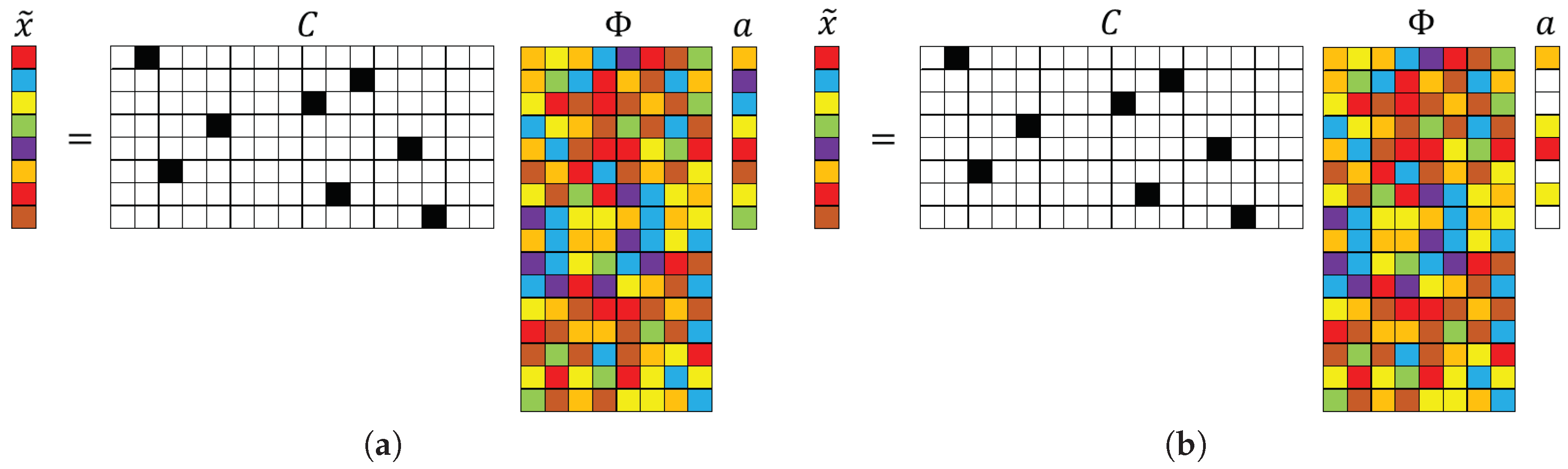
Figure 1. Schematic illustration of l 2 (a) and l 1 (b) minimization reconstruction for sparse recovery using a single-pixel measurement matrix. The numerical values in C are represented by colors: black (1), white (0). The other colors represent numbers that are neither 0 nor 1. In the above schematics x ˜ R P , C R P × N , Φ R N × N b and a R N b , where N b N . The number of colored cells in a represents the system sparsity K. K = N b for l 2 and K < N b for l 1 .
Fluids 03 00088 g001

(a)(b)
Figure 2. Schematic of the extreme learning machine (ELM) autoencoder network. In this architecture, the output features are the same as input features.
Fluids 03 00088 g002
Figure 3. Schematic of a gappy proper orthogonal decomposition (GPOD)-like sparse reconstruction (SR) formulation. The numerical values represented by the colored blocks are: black (1), white (0), color (other numbers).
Fluids 03 00088 g003
Figure 4. Isocontour plots of the stream-wise velocity component for cylinder flow at R e = 100 and T = 25 , 68 , and 200, showing the evolution of the flow field. Here, T represents the time non-dimensionalized by the advection time-scale.
Fluids 03 00088 g004
Figure 5. The temporal evolution of the first three normalized proper orthogonal decomposition (POD) coefficients for limit cycle cylinder flow at R e = 100 . (a) 2D view; (b) 3D view.
Fluids 03 00088 g005
Figure 6. Error ( e r r K P O D , e r r K E L M ) using different number of basis (K) for both POD reconstruction and ELM prediction.
Fluids 03 00088 g006
Figure 7. Isocontours of the normalized mean squared POD-based sparse reconstruction errors ( l 2 norms) using different random seeds (101 and 102) for sensor placements. Left: normalized absolute error metric, ϵ 1 . Right: normalized relative error metric, ϵ 2 . (a) ϵ 1 (seed = 101); (b) ϵ 2 (seed = 101); (c) ϵ 1 (seed = 102); and (d) ϵ 2 (seed = 102).
Fluids 03 00088 g007
Figure 8. Isocontours of the normalized mean squared POD-based sparse reconstruction errors ( l 2 norm) using different random seed (108 and 109) for sensor placements. Left: normalized absolute error metric, ϵ 1 . Right: normalized relative error metric, ϵ 2 . (a) ϵ 1 (seed = 108); (b) ϵ 2 (seed = 108); (c) ϵ 1 (seed = 109); and (d) ϵ 2 (seed = 109).
Fluids 03 00088 g008
Figure 9. Comparison of POD-based SR and full reconstruction (FR) for different random sensor placement and P K . Blue solid line: FR. Red dashed line: SR. Black stars: sensor locations. (a) Seed = 101 (at P = 3 and K = 3 ); (b) Seed = 102 (at P = 3 and K = 3 ); (c) Seed = 108 (at P = 2 and K = 3 ); and (d) Seed = 109 (at P = 2 and K = 3 ).
Fluids 03 00088 g009
Figure 10. Comparison of POD-based SR and FR for different random sensor placement and P > K . Blue solid line: FR. Red dashed line: SR. Black stars: sensor locations. (a) Seed = 101 (at P = 10 and K = 5 ); (b) Seed = 102 (at P = 10 and K = 5 ); (c) Seed = 108 (at P = 10 and K = 5 ); and (d) Seed = 109 (at P = 10 and K = 5 ).
Fluids 03 00088 g010
Figure 11. Isocontours of the normalized mean squared POD-based sparse reconstruction errors ( l 2 norm) corresponding to the sensor placement with maximum and minimum errors from the chosen ensemble of random sensor arrangements. The average error across the entire ensemble of ten random sensor placements is also shown. Left: normalized absolute error metric, ϵ 1 . Right: normalized relative error metric, ϵ 2 . (a) ϵ 1 (maximum); (b) ϵ 2 (maximum); (c) ϵ 1 (minimum); (d) ϵ 2 (minimum); (e) ϵ 1 (average); and (f) ϵ 2 (average).
Fluids 03 00088 g011
Figure 12. Isocontours of the normalized mean squared ( l 2 ) ELM-based sparse reconstruction errors for the maximum, minimum, and average using different choices of the random input weights. Left: normalized absolute error metric, ϵ 1 . Right: normalized relative error metric, ϵ 2 . (a) ϵ 1 (maximum); (b) ϵ 2 (maximum); (c) ϵ 1 (minimum); (d) ϵ 2 (minimum); (e) ϵ 1 (average); and (f) ϵ 2 (average).
Fluids 03 00088 g012
Figure 13. Isocontours of the normalized mean squared ( l 2 ) ELM-based sparse reconstruction error for maximum, minimum, and average error using different choices for the random sensor placement. Left: normalized absolute error metric, ϵ 1 . Right: normalized relative error metric, ϵ 2 . (a) ϵ 1 (maximum); (b) ϵ 2 (maximum); (c) ϵ 1 (minimum); (d) ϵ 2 (minimum); (e) ϵ 1 (average); and (f) ϵ 2 (average).
Fluids 03 00088 g013aFluids 03 00088 g013b
Table 1. The choice of sparse reconstruction algorithm based on problem design using parameters P (sensor sparsity), K (targeted system sparsity), and N b (candidate basis dimension).
Case K N b Relationship P K RelationshipAlgorithmReconstructed Dimension
1 K = N b P K l 2 K
2 K = N b P < K l 1 P
3 K < N b P < K < N b l 1 P
4 K < N b N b > P K l 1 K or P
5 K < N b P N b > K l 2 K or N b

