Symmetry Approach in the Evaluation of the Effect of Boundary Proximity on Oscillation of Gas Bubbles

Abstract

The purpose of the present review is to describe the effect of an interface between media with different mechanical properties on the acoustic response of a gas bubble. This is necessary to interpret sonar signals received from underwater gas seeps and mud volcanoes, as well as in the case of acoustic studies on the Arctic shelf where rising gas bubbles accumulate at the lower boundary of the ice cover. The ability to describe the dynamics of constrained bubble by analytical methods is related to the presence of internal symmetry in the governing equations. This leads to the presence of specific (toroidal and bi-spherical) coordinate systems in which the variables are separated. The existence of symmetry properties is possible only under certain conditions. In particular, the characteristic wavelength should be larger than the bubble size and the distance to an interface. The derived analytical solution allows us to determine how the natural frequency, radiation damping, and bubble shape depend on the distance to the boundary and the material parameters of contacting media.

1. Introduction

The presence of gas inclusions in the medium has a strong effect on the propagation of acoustic waves and leads to an additional damping and scattering of sound [1]. Hydro-acoustic manifestations of gas bubbles are important in various fields, such as acoustic oceanography, ultrasonic technologies, bio-medical applications. In the oil and gas industry, the detection of Leaks in sub-sea hydrocarbon pipelines and equipment represents a significant problem. At leakage, the gas bubbles are created and produce their birthing wails by which they can be identified [2].

Although a great deal is known about bubble oscillations in unbounded liquids [1], it is not very clear to what extent these results are applicable to the dynamics of constrained bubbles. Strasberg [3] was the first who studied the effect of a closely located rigid boundary boundary on the natural frequency of a single bubble. The effect of a rigid wall on gas bubble natural frequency has been evaluated in this approach by accounting for only monopole interactions between the bubble and its mirror image. The resonant frequency of a bubble attached to a solid boundary was first determined by Howkins [4]. The next step was done by Blue [5], who also adopted Strasberg’s theory to explain the experimental finding.

The experimental studies and a theoretical analysis of the behavior of in-phase oscillations of bubbles tethered to a plate have been performed by Paine et al. [6] and Illesinghe et al. [7]. The method of images developed by Strasberg [3] was used to model the effect of the boundary which, as noted above, requires correction at distances compared with the size of the bubble.

Microbubble contrast agents find application in a variety of biomedical technologies for imaging and drug delivery. In most cases, contrast agents perform forced oscillations near a boundary. Prediction of the natural frequency of the oscillation of ultrasound contrast agents in microvessels has drawn increasing attention [8,9,10]. Experimental studies demonstrate strong evidence that the microbubble oscillation amplitude and its back scattering signal amplitude are changed significantly if the contrast agent is in contact with the boundary. Garbin et al. [11] showed that the close proximity of a wall decreased the radial amplitude of microbubble oscillation by 50%. The influence of adherence at a wall on the dynamics of the microbubbles has been investigated by Overvelde et al. [12]. The shape of a bubble that performs volumetric oscillations can deform if it touches a wall. The amplitude of nonspherical oscillations of ultrasound contrast agent has been estimated by Vos et al. [13]. The nonspherical and translational behavior of individual microbubbles has been observed and categorized by Vos et al. [14]. The effect of the mechanical properties of adjoining media on the bubble dynamics remains poorly understood. It should be noted that there are experimental studies of the dynamic deformation of a viscoelastic layer induced by the volumetric oscillations of an ultrasound-driven microbubble [15], but there is no consistent theoretical explanation of the observed phenomena. A very comprehensive overview of achievements in this field has just become available [16]. The purpose of the series of studies [17,18,19,20,21] was to reveal how boundaries with different mechanical properties affect the acoustic response of a contrast agent microbubble. The radial motion of an encapsulated microbubble has been studied, taking into account only the monopole component in interaction. Since one of the purposes of these studies was a mechanism for sonoporation, the final calculations were performed at closest distances to the border. In this area, the corrections to the monopole contribution are the greatest.

The successes achieved with the use of numerical methods for simulating the behavior of a gas bubble located near a boundary were presented in the review by Blake and Gibson [22]. Further development of the method and new applications have been reported in subsequent works by Chahine et al. [23], Krasovitski and Kimmel [24], and Fong et al. [25].

The results presented in the current paper describe only linear phenomena in the interaction of a bubble with a boundary. For this reason, the description of a very complex mechanism of interaction of a laser-induced bubble with elastic materials observed experimentally [26,27,28], in particular, jetting formation, bubble migration, cavitation erosion, stress wave emission during optical breakdown and bubble collapse is currently possible only with the use of numerical methods.

A gas bubble is a very symmetrical object, which allows for a fairly complete description of its behavior even for a substantially nonlinear regime. The presence of confining surfaces located near the bubble disrupt the spherical symmetry of the problem and significantly limits the possibilities of analytical description. However, along with the physically obvious symmetry of the form, in this problem, there may exist less obvious but not less significant symmetries of the equations that describe the bubble behavior in the presence of constrains.

The application of methods of Lie groups consists in constructing geometric transformations of the space of independent and dependent variables of a system of differential equations. Almost for each important system of differential equations from the point of view of physics, these conditions of infinitesimal invariance are found [29] and allow, in particular, to predict coordinate systems in which the variables can be separated [30]. This approach has been used to obtain an analytical description of several phenomena in bubble dynamics [31,32,33,34]. The review surveys current studies and indicates issues for future research.

2. Results

Consider a bubble attached at the interface of a fluid (medium 1) with density ${\rho }_0$ and sound speed $c_0$ and the second medium characterized by density ${\rho }_{*}$ and sound speed $c_{*}$. The center of the bubble is at distance h from the boundary with the second medium. The basic bubble equilibrium shape consists of a bowl with the curvature $R_0$ (if the bubble is tethered to the interface $h<R_0$) and a sphere of radius $R_0$ (if the bubble is located at the distance $h>R_0$ from interface).

It will be assumed that the characteristic wavelengths of the acoustic field exceed the size of the bubble and the distance to the boundary $c_{0}T>>R_0,h$ (here T is the characteristic time scale), so that the liquid near the bubble wall can be regarded as incompressible. Under this condition, the velocity can be expressed as the gradient of a scalar potential $\phi$:

$$\mathit{v}=\nabla \phi ,{\nabla }^2\phi =0.$$

(1)

The relationship between pressure $P(\mathit{r},t)$ and potential in a liquid is determined by the Bernoulli integral

$$P(\mathit{r},t)+{\rho }_0\left[\dot{\phi }(\mathit{r},t)+\left(\nabla \phi ·\nabla \phi \right)/2-{\dot{\phi }}_{\infty }\left(t\right)\right]=P_{\infty }+P_m\left(t\right),$$

(2)

where $P_{\infty }$ is the equilibrium pressure in the liquid far from the bubble, $P_m\left(t\right)$ is the pressure in the acoustic wave. The potential in the Bernoulli equation is defined within an arbitrary function of time. For this reason, the potential at large distances from the bubble ${\phi }_{\infty }\left(t\right)$ is commonly taken to be zero. The amplitude of the bubble oscillation is assumed to be small. This allows one to neglect the nonlinear terms $\left(\nabla \phi ·\nabla \phi \right)/2$ in the Bernoulli equation.

The dynamic boundary condition expresses the balance of forces: the pressure on two sides of the bubble wall differ only because of surface tension:

$$P_l=P_g-\sigma \left(\nabla ·\mathit{n}\right),$$

(3)

where $P_l=P(\mathit{r}\in S,t)$ and $P_g=P_0{\left(V_0/V\right)}^{\gamma }$ denote the pressure in the liquid and in the bubble respectively, $\mathit{n}$ is the unit vector normal to the bubble surface $S_0$, $\sigma$ is the coefficient of surface tension of the gas/liquid interface. We adopt a widely used equation of state for gas in a bubble corresponding to a polytropic law, V, $V_0$ are the instantaneous and equilibrium bubble volume, $\gamma$ is the polytropic exponent, $P_0$ is the equilibrium pressure in the bubble.

The kinematic boundary condition expresses continuity of displacements on the bubble wall:

$$\dot{\zeta }={\left(\mathit{v}·\mathit{n}\right)}_{\mathit{r}\in S_0},$$

(4)

where $\zeta$ is the normal displacement of the bubble wall $S_0$.

The pressure in the acoustic wave can be considered spatially uniform at a distance less than characteristic wavelength. For this reason, the assumption that the bubble possesses axial symmetry and has no angular momentum will be justified. The choice of a particular coordinate system will help us to find an analytical solution to the problem. This coordinate system should have axial symmetry and lead to the separation of variables in the Laplace equation.

2.1. Symmetries in the Dynamics of Constrained Bubble

The Laplace Equation (1) is very symmetric. It is clearly invariant under translations, rotations, and scaling transformations. The full set of infinitesimal generators of symmetries for this equation have the following form [30]

$$\begin{array}{c}\hfill P_j={\partial }_j={\partial }_{xj},j=1,2,3;J_1=x_3{\partial }_2-x_2{\partial }_3,J_2=x_1{\partial }_3-x_2{\partial }_1,J_3=x_2{\partial }_1-x_1{\partial }_2;K_1=x_1\\ \hfill +\left(x_1^2-x_2^2-x_3^2\right){\partial }_1+2x_1{x}_3{\partial }_3+2x_1{x}_2{\partial }_2,K_2=x_2+\left(x_2^2-x_1^2-x_3^2\right){\partial }_2+2x_2{x}_3{\partial }_3+2x_1{x}_2{\partial }_1,\\ \hfill K_3=x_3+\left(x_3^2-x_1^2-x_2^2\right){\partial }_3+2x_1{x}_3{\partial }_1+2x_1{x}_2{\partial }_2;D=-\left(1/2+x_1{\partial }_1+x_2{\partial }_2+x_3{\partial }_3\right),\end{array}$$

(5)

where $P_j$ are the generators of translations, $J_j$ are the generators of rotations, D is the generator of dilatations and the $K_j$ are generators of special conformal transformations. The tenth-dimensional algebra of symmetry of the Laplace Equation (5) leads to 17 coordinate systems, enabling the separation of variables [30]. The toroidal and bi-spherical coordinates are part of these systems.

For most important linear equations, solutions with separating variables are common eigenfunctions of second order commuting operators from the enveloping Lie algebra of symmetries corresponding to this equation. The commuting symmetry operators that completely specify the toroidal coordinates are $S_1=J_3^2$ and $S_2={\left(P_3+K_3\right)}^2$ [30].

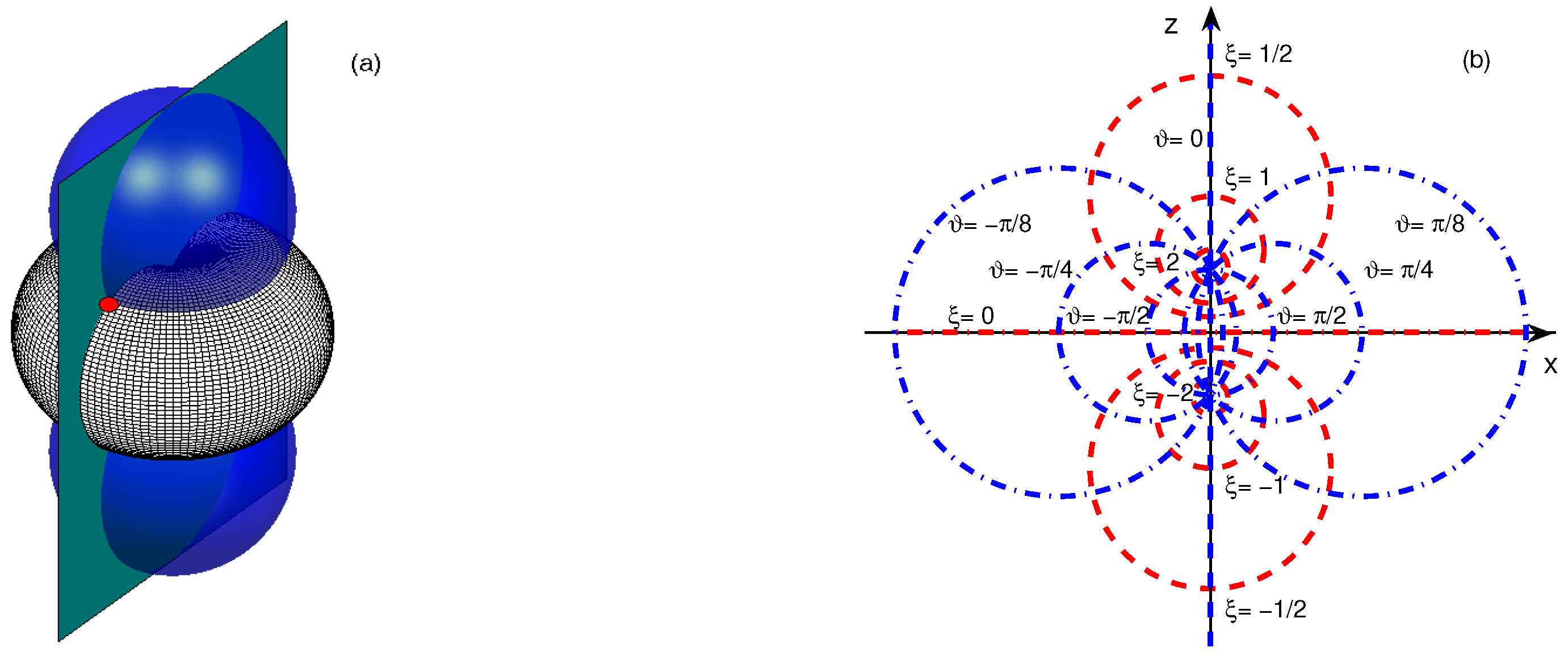
The toroidal coordinates ($\eta ,\psi ,\alpha$) are related with Cartesian ones ($x,y,z$) by the relations:

$$x=\frac{L}{2}\frac{sinh\eta cos\alpha }{cosh\eta -cos\psi },y=\frac{L}{2}\frac{sinh\eta sin\alpha }{cosh\eta -cos\psi },z=\frac{L}{2}\frac{sin\psi }{cosh\eta -cos\psi },$$

(6)

where $\eta$ goes from 0 to ∞, $\psi$ and $\alpha$ go from $-\pi$ to $\pi$ and from 0 to $2\pi$, correspondingly; L is the diameter of the focal ring. The surface $\eta =\mathrm{const}$ is a torus and the surface $\psi =\mathrm{const}$ is a spherical bowl. An illustration of toroidal coordinates is shown in Figure 1a,b. The system of toroidal coordinates is orthogonal.

2.2. Dynamics of a Tethered Bubble

Toroidal coordinates is a natural coordinate system for analysis of oscillations of tethered bubbles since the equilibrium surface of a such bubble is a spherical bowl. The Laplace equation has the following form in toroidal coordinates

$$\frac{1}{h_{\eta }^3}\left[\frac{1}{sinh\eta }\frac{\partial }{\partial \eta }{h}_{\eta }sinh\eta \frac{\partial }{\partial \eta }+\frac{\partial }{\partial \psi }{h}_{\psi }\frac{\partial }{\partial \psi }+\frac{h_{\alpha }}{sinh\eta }\frac{{\partial }^2}{\partial {\alpha }^2}\right]\phi \left(\eta ,\psi ,\alpha ,t\right)=0,$$

(7)

where $h_{\eta }=h_{\psi }=\left(L/2\right){\left[cosh\eta -cos\psi \right]}^{-1}$, $h_{\alpha }=\left(L/2\right)sinh\eta {\left[cosh\eta -cos\psi \right]}^{-1}$ are the Lamè coefficients.

The boundary conditions to this equation should be specified on the bubble wall ${\psi }_w={\theta }_c$ (where ${\theta }_c$ is the contact angle) and on the boundary ${\psi }_b=0$ which corresponds to the interface (see Figure 1). The relation between the diameter of the ring of contact L and the equilibrium radius of the bubble $R_0$ is given by $L=2R_{0}sin{\theta }_c$.

To separate the variables in the Laplace equation, we replace $\phi \left(\eta ,\psi ,\alpha ,t\right)$ by $\sqrt{cosh\eta -cos\psi }\tilde{\phi }\left(\eta ,\psi ,\alpha ,t\right)$ [35]. In view of the axial symmetry of the system, Equation (7) acquires the form

$$\left[\widehat{L}+\frac{{\partial }^2}{\partial {\psi }^2}\right]\tilde{\phi }(\eta ,\psi ,t)=0,\widehat{L}\tilde{\phi }=\frac{1}{sinh\eta }\frac{\partial }{\partial \eta }sinh\eta \frac{\partial }{\partial \eta }\tilde{\phi }+\frac{\tilde{\phi }}{4},$$

(8)

here $\tilde{L}$ is the Legendre operator. An important class of integral expansions involving spherical harmonics is commonly known as Mehler-Fock integral transforms. This suggests that the solution of Equation (8) can be found in the form [36]:

$$\tilde{\phi }(\eta ,\psi )={\int }_0^{\infty }{P}_{-1/2+i\tau }(cosh\eta )\Phi (\psi ,\tau )d\tau ,$$

(9)

$$\Phi (\psi ,\tau )=\tau tanh\left(\pi \tau \right){\int }_0^{\infty }{P}_{-1/2+i\tau }(cosh\eta )\tilde{\phi }(\eta ,\psi )sinh\eta d\eta .$$

(10)

Equations (9) and (10) represent the forward and inverse transformations. Here, $P_{-1/2+i\tau }(cosh\eta )$ is the Legendre functions of the first kind. The degree of the associated Legendre function appears as the integration variable in the inversion formula.

The kernel of the integral transform, $\Phi (\psi ,\tau )$, obeys the equation

$$\frac{{\partial }^2\Phi (\psi ,\tau )}{\partial {\psi }^2}={\tau }^2\Phi (\psi ,\tau ).$$

(11)

The substitution of the solution of Equation (11) into Equation (9) yields the general form of the required solution

$$\tilde{\phi }(\eta ,\psi )={\int }_0^{\infty }\left[a\left(\tau \right)cosh\left(\psi \tau \right)+b\left(\tau \right)sinh\left(\psi \tau \right)\right]P_{-1/2+i\tau }(cosh\eta )d\tau ,$$

(12)

where $a\left(\tau \right)$ and $b\left(\tau \right)$ should be determined from the boundary conditions on the bubble wall.

We shall assume that the characteristic length of the acoustic wave exceeds the dimensions of the bubble not only in the liquid, but also in the gas. Under these conditions, the pressure inside the bubble will change periodically in time, but remain spatially homogeneous. It follows from the Bernoulli equation that the surface of such a homobaric bubble will be equipotential, if neglecting surface tension and nonlinear term. We shall analyze only linear volume oscillations of the relatively large bubbles and therefore can use this approximation $\phi {(\eta ,\psi ,t)}_{\psi ={\theta }_c}={\phi }_0\left(t\right)$.

For the relatively simple case when the lower medium is absolutely rigid $\left({\partial \phi /\partial \psi |}_{\psi =0}=0\right)$ we have $b\left(\tau \right)=0$. After using the Heine identity [36]

$$\frac{1}{\sqrt{cosh\eta -cos{\theta }_c}}=\sqrt{2}{\int }_0^{\infty }\frac{cosh\left[(\pi -{\vartheta }_c)\tau \right]}{cosh\left(\pi \tau \right)}{P}_{-1/2+i\tau }(cosh\eta )d\tau ,$$

(13)

one obtains

$$a\left(\tau \right)={\phi }_0\left(t\right)\sqrt{2}\frac{cosh\left[(\pi -{\vartheta }_c)\tau \right]}{cosh\left(\pi \tau \right)cosh\left(\vartheta \tau \right)}$$

(14)

which provides finding in the close form the solution of the problem:

$$\phi (\eta ,\psi ,t)={\phi }_0\left(t\right){\left(cosh\eta -cos\psi \right)}^{1/2}\sqrt{2}{\int }_0^{\infty }\frac{cosh\left(\psi \tau \right)cosh\left[(\pi -{\vartheta }_c)\tau \right]}{cosh\left(\pi \tau \right)cosh\left({\vartheta }_c\tau \right)}{P}_{-1/2+i\tau }(cosh\eta )d\tau .$$

(15)

The Legendre function of complex index could be expressed by means of the following integral

$$P_{-1/2+i\tau }(cosh\eta )=\frac{\sqrt{2}}{\pi }coth\left(\pi \tau \right){\int }_{\eta }^{\infty }dt\frac{sin\left(t\tau \right)}{{\left(cosht-cosh\eta \right)}^{1/2}}.$$

(16)

Substitution of this expression into Equation (15) allows one to convert it to the form

$$\phi (\eta ,\psi ,t)={\phi }_0\left(t\right)\left[1-{\left(cosh\eta -cos\psi \right)}^{1/2}\frac{2}{{\vartheta }_c}{\int }_{\eta }^{\infty }\frac{cos\left(\frac{\psi \pi }{2{\vartheta }_c}\right)sinh\left(\frac{t\pi }{2{\vartheta }_c}\right)dt}{{\left(cosht-cosh\eta \right)}^{1/2}\left[cosh\left(\frac{t\pi }{{\vartheta }_c}\right)-cos\left(\frac{\psi \pi }{{\vartheta }_c}\right)\right]}\right].$$

(17)

In this form, the behavior of the potential in the vicinity of the tethered bubble was derived earlier [37]. However, the method by which these results were obtained was complicated and of an intuitive, rather than a regular nature. By using the transformation of inversion relative to the ring of contact, the original problem has been reduced to the form corresponding to the field of point charge in the wedge. The inverse transformation of the known solution of electrostatics led to Equation (17). A small difference between the earlier [37] and the present approaches consists in using the different boundary conditions for the potential at the bubble wall ${\phi }_0\left(t\right)$ and far from the bubble ${\phi }_{\infty }\left(t\right)$: it was assumed in the Ref. [37] that ${\phi }_0\left(t\right)=0$, ${\phi }_{\infty }\left(t\right)\ne 0$ but we set ${\phi }_0\left(t\right)\ne 0$, ${\phi }_{\infty }\left(t\right)=0$ in the present approach. This difference is not important, since the potential is determined to within an arbitrary function of time.

Substitution of solutions in the form of (15) and (17) into the kinematic boundary condition Equation (4) establishes the relationship between the time variation in the bubble volume $\Delta \dot{V}$ and the value of the potential at the bubble wall ${\phi }_0\left(t\right)$

$$\begin{array}{c}\hfill \Delta \dot{V}=LC{\phi }_0\left(t\right),\\ \hfill C={\left(1-cos\left({\vartheta }_c\right)\right)}^{1/2}\frac{\pi }{{\vartheta }_c}{\int }_0^{\infty }\frac{sinht}{\left(cosht-cos\left({\vartheta }_c\right)\right)cosh\left(\frac{t\pi }{2{\vartheta }_c}\right)\left(cosht-1\right)}dt\\ \hfill =\left(2\pi \right){\int }_0^{\infty }d\tau \frac{cosh\left[\left(\pi -{\vartheta }_c\right)\tau \right]}{cosh\left(\pi \tau \right)cosh\left({\vartheta }_c\tau \right)}.\end{array}$$

(18)

Introducing the notation C (capacity), we use the existing analogy of dynamics of homobaric bubble and electrostatics [38]. The form of Equation (18) substantially simplifies the expression given in Ref. [37] where C was described by a double integral. Different forms of representation for C correspond to the two forms of the solution found Equations (15) and (17). When performing numerical calculations, the third line of Equation (18) is useful. In turn, the form presented on the second line of Equation (18) is more convenient for the discovery of the fact that the integral for C can be reduced to analytical formulas for definite values of wetting angles: ${\vartheta }_c=\pi /6,\pi /4,\pi /3,\pi /2$ [37].

Substituting ${\dot{\phi }}_0\left(t\right)$ expressed through the change of volume in the dynamic boundary condition (3), we obtain an analogue of the Rayleigh equation [37]

$$\frac{1}{2R_{0}sin{\vartheta }_{c}C\left({\vartheta }_c\right)}\frac{d^2\Delta V}{d{t}^2}+\frac{\gamma P_0}{{\rho }_0{V}_0}\Delta V=-\frac{P_m}{{\rho }_0}sin\left(\omega t\right).$$

(19)

It follows directly from this equation that the fundamental frequency of the tethered bubble has the form

$${\Omega }_{*}^2\left(R_0,{\vartheta }_c\right)=\frac{2\gamma R_{0}sin{\vartheta }_{c}C\left({\vartheta }_c\right)P_0}{{\rho }_0{V}_0}={\Omega }_0^2\frac{sin{\vartheta }_{c}C\left({\vartheta }_c\right)}{2\pi \left[1-\frac{{\left(1-cos{\vartheta }_c\right)}^2(2+cos{\vartheta }_c)}{4}\right]},$$

(20)

where ${\Omega }_0={\left[\left(3\gamma P_0\right)/\left({\rho }_0{R}_0^2\right)\right]}^{1/2}$ is the fundamental frequency of a free bubble of the same radius of curvature $R_0$. The ratio of these frequencies $\tilde{\Omega }={\Omega }_{*}/{\Omega }_0$ depends only on ${\vartheta }_c$. The plot of the dependence $\tilde{\Omega }$ on ${\vartheta }_c$ presented in the Ref. [37] is the only predicted physical effect that can be verified experimentally. This is an obvious defect in the developed approach. However, the unified approach based on the use of toroidal coordinates makes it possible to significantly expand this list. Thus, some of the effects described in the next section, related to the analysis of the behavior of the bubbles located at a close distance from the boundary surface in bi-spherical coordinates, have a close analogues for a tethered bubbles, which can be studied in toroidal coordinates.

2.3. Bubble Dynamics Close to Interface

In this section, we use a bi-spherical coordinate system for separating variables in the Laplace equation. In contrast to toroidal coordinates, this system is conformally equivalent to a system of spherical coordinates. However, these two coordinate systems are not equivalent with respect to the Euclidean group [30].

The bi-spherical coordinates ($\xi ,\vartheta ,\alpha$) are related to Cartesian coordinates ($x,y,z$) by the relations:

$$\begin{array}{c}\hfill x=a\frac{sin\vartheta cos\alpha }{cosh\xi -cos\vartheta },y=a\frac{sin\vartheta sin\alpha }{cosh\xi -cos\vartheta },z=a\frac{sinh\xi }{cosh\xi -cos\vartheta },\\ \hfill a=R_{0}sinh{\xi }_0,{\xi }_0=ln\left[h/R_0+\sqrt{{\left(h/R_0\right)}^2-1}\right],\end{array}$$

(21)

where $\xi$ goes from $-\infty$ to ∞, $\vartheta$ and $\alpha$ go from 0 to $\pi$ and from 0 to $2\pi$, correspondingly. The surface $\xi ={\xi }_0$ is the bubble, while the interface corresponds to $\xi =0$. For $\xi =0$, $cos\vartheta \to 1$ corresponds to $r\to \infty$. Illustration of the bi-spherical coordinate system is shown in Figure 2a,b.

By its structure, the Laplace equation in bi-spherical coordinates is close to Equation (7) and has the following form

$$\begin{array}{c}\hfill {\nabla }^2\phi =\frac{1}{h_{\xi }^3}\left[\frac{1}{sin\vartheta }\frac{\partial }{\partial \vartheta }\left(h_{\vartheta }sin\vartheta \frac{\partial \phi }{\partial \vartheta }\right)+\frac{\partial }{\partial \xi }\left(h_{\xi }\frac{\partial \phi }{\partial \xi }\right)+\frac{h_{\alpha }}{{sin}^2\vartheta }\frac{{\partial }^2\phi }{\partial {\alpha }^2}\right]=0,\\ \hfill h_{\xi }=h_{\vartheta }=a{\left[cosh\xi -cos\vartheta \right]}^{-1},h_{\alpha }=asin\vartheta {\left[cosh\xi -cos\vartheta \right]}^{-1},\end{array}$$

(22)

where $h_{\xi }$, $h_{\vartheta }$, $h_{\alpha }$ are the Lamè coefficients.

A solution procedure for the Laplace equation in bi-spherical coordinates requires the introduction of the following substitution: $\phi =\sqrt{cosh\xi -cos\vartheta }\tilde{\phi }$. In view of the assumed axial symmetry, the function $\tilde{\phi }$ does not depend on the azimuthal angle. For the function $\tilde{\phi }$, the variables are separated.

We begin with the simplest solution [39] obeying rigid boundary conditions. Applying the equipotentiality condition ${\phi (\xi ,\vartheta ,t)|}_{\xi ={\xi }_0}={\phi }_0\left(t\right)$ on the bubble wall and the impermeability condition on the rigid boundary $h_{\xi }^{-1}{\left(\partial \phi /\partial \xi \right)}_{\xi =0}=0$, we find the analytic solution of the boundary value problem

$$\begin{array}{c}\hfill \phi (\xi ,\vartheta ,t)={\phi }_0\left(t\right)\sqrt{cosh\xi -cos\vartheta }\sqrt{2}\sum _{n=0}^{\infty }{P}_n(cos\vartheta )e^{-(n+1/2){\xi }_0}\frac{cosh\left[(n+1/2)\xi \right]}{cosh\left[(n+1/2){\xi }_0\right]},\end{array}$$

(23)

here $P_n(cos\vartheta )$ are the Legendre functions. The structure of Equation (23) is similar to that obtained in Ref. [40] for the free surface and corresponds to another limiting case, that of a rigid boundary.

The time derivation of the bubble volume, $\Delta \dot{V}$, can be expressed through the potential at the bubble wall

$$\begin{array}{c}\hfill \frac{\Delta \dot{V}}{V_0}=-\frac{3{\phi }_0\left(t\right){\tilde{\Omega }}^2\left(\kappa \right)}{R_0^2},\kappa =\frac{h}{R_0},{\tilde{\Omega }}^2=1-2\sqrt{{\kappa }^2-1}\sum _{n=0}^{\infty }\frac{{\left[\kappa +\sqrt{{\kappa }^2-1}\right]}^{-(2n+1)}}{{\left[\kappa +\sqrt{{\kappa }^2-1}\right]}^{(2n+1)}+1}.\end{array}$$

(24)

Substitution of this relation into the dynamic boundary condition (3) leads to the Rayleigh equation for the volume variation $\Delta V\left(t\right)$

$$\Delta \ddot{V}+{\Omega }_{0*}^2\Delta V=0,{\Omega }_{0*}=\tilde{\Omega }{\Omega }_0.$$

(25)

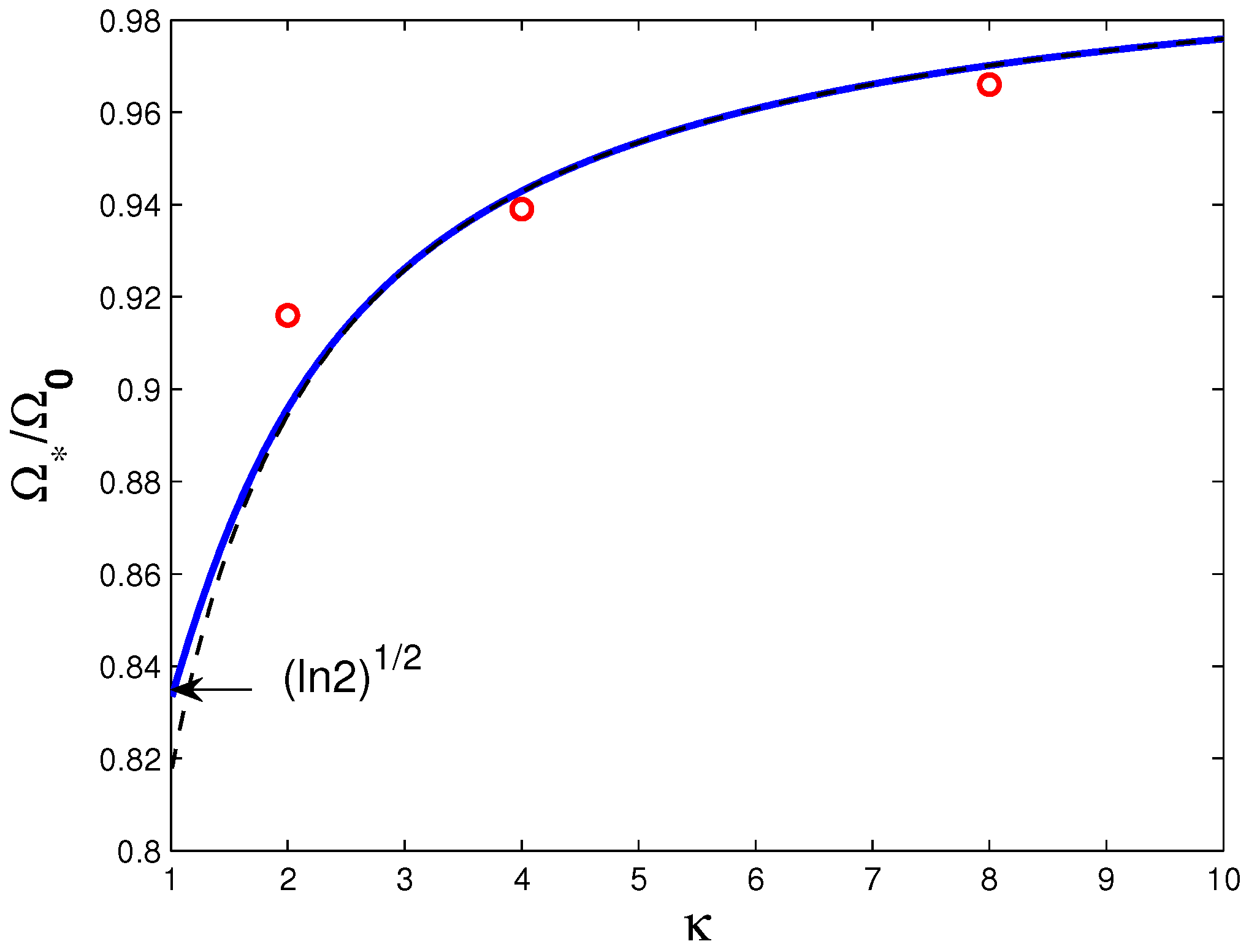
Here, ${\Omega }_{0*}$ is the natural frequencies of the bubble located at the distance h above the rigid bottom. A graph of the ratio ${\Omega }_{*}/{\Omega }_0$ as function of $h/R_0$ is shown in Figure 3 of the Ref. [39].

The presence of a rigid boundary decreases the natural frequency. The figure also includes a comparison of these calculated values with measured values. There is a continuous transition from the state of the tethered bubble to the state of the bubble located at some distance from the surface. This is the state of the bubble which touches the surface at one point. The shift of the natural frequency obtained for this case [37] and the results of the Ref. [39], which uses bi-spherical coordinates, give the same value.

The problem of describing the dynamics of a bubble located at some distance from the boundary is much simpler than the description of a tethered bubble, since it does not require analysis of the behavior in the vicinity of the contact line. For this reason, a much more detailed study of the features of the behavior of such an inclusion can be obtained.

First, we consider the acoustic correction to the incompressible Rayleigh-Plesset Equation (25). The implementation of this procedure follows the approach suggested by [41,42] and account for the presence of the rigid boundary. The radiation damping results from the emission of energy away from the bubble as sound. Use is made of the method of matched asymptotic expansion in which the small parameter is $ϵ=R_0/\left(c_0{T}_0\right)$. In this way we find [39]

$$\Delta \ddot{V}+{\nu }_r\Delta \dot{V}+{\Omega }_{0*}^2\Delta V=0,{\nu }_r=\frac{2R_0{\tilde{\Omega }}^2{\Omega }_{0*}^2}{c_0}.$$

(26)

The damping constant ${\gamma }_r$ differs from that for a free bubble by a co-factor $\left(2{\tilde{\Omega }}^4\right)$. Since the presence of a rigid wall doubles the amplitude of potential in the far field, then the power (which is proportional to the square of the amplitude) leads to the factor 4. However, the radiation from the bubble near the rigid wall occurs only in a half of the solid angle. For this reason, only the factor 2 enters into the final expression for the radiation damping. This result is valid only for the case when the wavelength is much greater than the distance to the rigid wall $\lambda >>h$ and one can ignore the phase difference between the direct wave and the one reflected from the wall. The factor ${\tilde{\Omega }}^4$ reflects the variation in the bubble inertial mass near the wall. This term quickly approaches unity with increasing distance from the bubble to the wall.

So far, we have assumed the flow near the bubble and the rigid wall to be inviscid and irrotational. In reality, the presence of viscosity implies that the tangential and normal components of the stress must be continuous at the surface of the bubble. The velocity should be vanished at the rigid wall. To accommodate these boundary conditions other types of solution of the viscous equations of motion are required. For the millimeter sized bubbles and kHz frequency range, the viscous length $\left|\delta \right|$, (${\delta }^{-1}={\left(-\mathrm{i}\omega /\nu \right)}^{1/2})$ is small compared with the equilibrium radius $R_0$. Thus vorticity is restricted to the thin boundary layers near the bubble interface and the rigid wall.

A straightforward method for taking into account the vorticity would be to proceed by successive approximations. On the other hand, if we restrict our analysis to finding the value of viscous damping, and not the details of flow in the near interface region, we can use the approach based on the total energy conservation in incompressible liquid. In this approach, time derivative of energy is balanced by dissipative function. Longuet-Higgins [43] used this approach in finding viscous damping of surface modes on the bubble wall. As was shown in Ref. [39], the damping factor of bubble oscillations due to dissipation near the boundary has the form

$${\gamma }_v=\frac{2\nu }{R_0^2}\frac{R_0}{\left|\delta \right|{\tilde{\Omega }}^2}{F}_v\left(\kappa \right).$$

(27)

One can identify three factors in this expression. The first one $2\nu /R_0^2$ characterizes the viscous losses at the free surface—the bubble wall. The second factor shows how the viscous losses near the rigid wall exceed the losses at the free surface $R_0/\left|\delta \right|>>1$. The third factor $F_v\left(\kappa \right)$ describes the law of diminishing losses with increasing the distance from the bubble to the rigid wall $\kappa =h/R_0$. The explicit form of $F_v$ is given in Ref. [39]. For large values of the argument $\kappa$ $\left(h>>R_0\right)$ $F_v$ is given by the formula $F_v\approx {\left(4{\kappa }^2\right)}^{-1}$. Figure 4 illustrates the behavior of $F_v$ on $\kappa =h/R_0$ for the most interesting range of distances. The starting point is the state when the bubble near touches the boundary, and then this interval extends up to a relatively large distances ($\kappa =10$, $h=10R_0$).

Please note that although the surface value of the potential over the bubble wall is constant, the value of the normal derivative, which determines the displacement and deformation of the bubble shape $\zeta =h_{\xi }^{-1}{\left(\partial \phi /\partial \xi \right)}_{\xi ={\xi }_0}$, varies with the angle $\vartheta$. To illustrate the variation in the bubble shape during its oscillations near the rigid wall, the angular dependence of the displacement $\zeta$ on $\vartheta$ has been evaluated [39].

Figure 5 shows the distortions reached during the expansion (dashed line) and contraction (dot-dashed line) phases of oscillations, for the dimensionless amplitude $\zeta /R_0={\phi }_0\left(0\right)/\left({\Omega }_{*}{R}_0^2\right)=0.2$. The bubble equilibrium shape is shown by the the solid line. The dependencies shown in the figure demonstrate a rather non-obvious fact that the bubble shape can be qualitatively well described by the first terms of the multipole expansion even at a relatively short distance from the boundary. This approach provides an efficient way to evaluate the accuracy of the approximate methods [17,18]. In applying these methods it was assumed that the bubble undergoes only radial and translational oscillations near an interface.

The interaction of a bubble with a boundary is traditionally taken into account by introducing a mirror monopole source. The applicability of this method is restricted by the condition of smallness of the bubble size compared to the distance to the bounding surface. An approach using specific coordinate systems for separating variables was successfully used in describing the behavior of tethered inclusions and bubbles located near rigid boundaries. The boundary of most media is not absolutely rigid, so the next step in applying the method is to examine the bubble behavior near an interface between two liquids.

2.4. Bubble Oscillations Near an Interface between Two Liquids

In this case, the parameters of the second medium—its density and the speed of sound—influence the behavior of the bubble. At the interfaces, the boundary conditions should be satisfied, which include continuity of displacements and equality of forces. In each medium, the potential satisfies the Helmholtz equation. However, if we use the integral representation of this equation, this will make it possible to express the potential in the medium (1), where the bubble is located, through the boundary values on the interfaces:

$$\phi \left(\mathbf{r}\right)=\frac{1}{4\pi }{\int }_{S_0+S_{int}}\left[G(\mathbf{r},{\mathbf{r}}^{\prime })\frac{\partial \phi \left({\mathbf{r}}^{\prime }\right)}{\partial n^{\prime }}-\phi \left({\mathbf{r}}^{\prime }\right)\frac{\partial G(\mathbf{r},{\mathbf{r}}^{\prime })}{\partial n^{\prime }}\right]dS,$$

(28)

where $G(\mathbf{r},{\mathbf{r}}^{\prime })$ is the Green’s function, $\mathbf{r}$ is the position of the observation point, ${\mathbf{r}}^{\prime }$ corresponds to points at the bubble surface and interface and $\partial /\partial n^{\prime }$ is the derivative with respect to the normal (the normal is directed inside the bubble and inside medium (2)).

In the first stage [44], we will analyze natural bubble oscillations, and, therefore, the right-hand side of Equation (28) does not contain the term describing the source. The choice of the Green’s function in Equation (28) makes it possible to simplify considerably the procedure for finding the solution. Following [45], we choose it in the form satisfying the boundary conditions at the interface between two liquids. For a planar interface, this leads to the fact that the integral over $S_{int}$ vanishes, so that only the integral over the bubble surface remains in Equation (28).

When solving Equation (28), we use the asymptotic expansion method, with the small parameter being the ratio $ϵ$ of the bubble size and the bubble-to-boundary distance to the wavelength. In the vicinity of the bubble, $r\approx R_0,h$, the media can be considered incompressible. Far from the bubble, $r\approx (c_0,c\ast )T$, the finite speed of propagation is essential.

$$\begin{array}{c}\hfill \phi \left(\mathbf{r}\right)={\phi }_0\left(\mathbf{r}\right)+ϵ{\phi }_1\left(\mathbf{r}\right)+\dots ,\\ \hfill G(\mathbf{r},{\mathbf{r}}^{\prime })=G_0(\mathbf{r},{\mathbf{r}}^{\prime })+ϵG_1(\mathbf{r},{\mathbf{r}}^{\prime })+\dots \end{array}$$

(29)

We will take into account only two first terms of the series expansion, which, as shown by Prosperettit [41], is sufficient to determine the natural frequency and the radiation damping of bubble oscillations.

The zero-order and first-order equations have the form

$$\begin{array}{c}\hfill {\phi }_0\left(\mathbf{r}\right)=\frac{1}{4\pi }{\int }_{S_0}\left[G_0(\mathbf{r},{\mathbf{r}}^{\prime })\frac{\partial {\phi }_0\left({\mathbf{r}}^{\prime }\right)}{\partial n^{\prime }}-{\phi }_0\left({\mathbf{r}}^{\prime }\right)\frac{\partial G_0(\mathbf{r},{\mathbf{r}}^{\prime })}{\partial n^{\prime }}\right]dS,\\ \hfill {\phi }_1\left(\mathbf{r}\right)=\frac{1}{4\pi }{\int }_{S_0}\left[G_0(\mathbf{r},{\mathbf{r}}^{\prime })\frac{\partial {\phi }_1\left({\mathbf{r}}^{\prime }\right)}{\partial n^{\prime }}+G_1(\mathbf{r},{\mathbf{r}}^{\prime })\frac{\partial {\phi }_0\left({\mathbf{r}}^{\prime }\right)}{\partial n^{\prime }}-{\phi }_0\left({\mathbf{r}}^{\prime }\right)\frac{\partial G_1(\mathbf{r},{\mathbf{r}}^{\prime })}{\partial n^{\prime }}-{\phi }_1\left({\mathbf{r}}^{\prime }\right)\frac{\partial G_0(\mathbf{r},{\mathbf{r}}^{\prime })}{\partial n^{\prime }}-\right]dS.\end{array}$$

(30)

This system of equations becomes completely defined if we supplement it with the boundary conditions at the bubble wall Equations (3) and (4).

The first two terms of the expansion of the Green’s function that appear in Equations (30) have the form [44]:

$$\begin{array}{c}\hfill G_0(\mathbf{r},{\mathbf{r}}^{\prime })=\frac{1}{|\mathbf{r}-{\mathbf{r}}^{\prime }|}+\frac{1}{|\mathbf{r}-{\mathbf{r}}^{\prime }+2z^{\prime }{\mathbf{e}}_z|}\frac{m-1}{m+1},G_1(\mathbf{r},{\mathbf{r}}^{\prime })=2i{k}_{0}m\left[\frac{m-n}{m^2+1}+mC(n,m)\right],\\ \hfill C(n,m)=\left\{\begin{array}{cc}-\frac{{(n^2-1)}^{1/2}}{{(m^2-1)}^{3/2}}ln\left[\frac{\left(1-\sqrt{\frac{(n-1)(m-1)}{(n+1)(m+1)}}\right)}{\left(1+\sqrt{\frac{(n-1)(m-1)}{(n+1)(m+1)}}\right)}\right],\hfill & n>1,m>1;\hfill \\ -\frac{2{(n^2-1)}^{1/2}}{{(1-m^2)}^{3/2}}arctan\left[\sqrt{\frac{(n-1)(1-m)}{(n+1)(m+1)}}\right],\hfill & n>1,m<1;\hfill \\ -\frac{2{(1-n^2)}^{1/2}}{{(m^2-1)}^{3/2}}arctan\left[\sqrt{\frac{(1-n)(m-1)}{(n+1)(m+1)}}\right],\hfill & n<1,m>1;\hfill \\ -\frac{{(1-n^2)}^{1/2}}{{(1-m^2)}^{3/2}}ln\left[\frac{\left(1-\sqrt{\frac{(1-n)(1-m)}{(n+1)(m+1)}}\right)}{\left(1+\sqrt{\frac{(1-n)(1-m)}{(n+1)(m+1)}}\right)}\right],\hfill & n<1,m<1.\hfill \end{array}\right.\end{array}$$

(31)

where ${\mathbf{e}}_z$ is the unit vector along the z axis, $m={\rho }_{*}/{\rho }_0$, $n=c_0/c_{*}$. The zero-order Green’s function can be interpreted as follows: it consists of two monopole sources in an incompressible liquid, namely, a direct source and a mirror one with respect to the interface, the mirror source intensity being such that the boundary conditions are satisfied. The first-order Green’s function $G_1$ is constant and independent of spatial coordinates. It should be noted that the above formulas are valid within the wave zone.

To find the zero-approximation solution ${\phi }_0\left(\mathbf{r}\right)$, we use the fact that the liquid within the wave zone near the bubble can be considered incompressible. This means that the potential is a solution of the Laplace equation along with the integral equation (the first lune of Equation (30)). The convenience of the integral equation is that we do not need to worry about satisfying the boundary conditions at the interface $S_{int}$. It suffices to substitute a general solution to the Laplace equation and explicit form of the Green’s function into the integral equation. Thus, the zero-approximation solution takes on the form [44]:

$${\phi }_0(\xi ,\vartheta )=\sqrt{cosh\xi -cos\vartheta }{\phi }_0\left(\omega \right)\sqrt{2}{\sum }_{k=0}^{\infty }{e}^{-(k+1/2){\xi }_0}\frac{(m+1)e^{(k+1/2)\xi }+(m-1)e^{-(k+1/2)\xi }}{(m+1)e^{(k+1/2){\xi }_0}+(m-1)e^{-(k+1/2){\xi }_0}}{P}_k(cos\vartheta ).$$

(32)

The solution to the first-approximation is independent of spatial coordinates and has the form [44]

$$\begin{array}{c}\hfill {\phi }_1=i{k}_0{\phi }_0\left(\omega \right)2m\left[\frac{m-n}{m^2+1}+mC(n,m)\right]{\Omega }_b^2,\\ \hfill {\Omega }_b^2=1-2sinh{\xi }_0\sum _{k=0}^{\infty }\frac{(m-1)e^{-(2k+1){\xi }_0}}{(m+1)e^{(2k+1){\xi }_0}+(m-1)}.\end{array}$$

(33)

This leads [44] to the modified Rayleigh Equation (26) in which the frequency ${\Omega }_{0*}$ is replaced by ${\Omega }_{*b}$ and ${\nu }_r$ is replaced by $\nu$

$${\Omega }_{*b}={\Omega }_0{\Omega }_b,\nu =\left({\Omega }_0^2{R}_0/c_0\right)2m\left[\frac{m-n}{m^2+1}+mC(n,m)\right]{\Omega }_b^4.$$

(34)

Spatial variations of ${\Omega }_{*b}$ and $\nu$ are governed by the behavior of factor ${\Omega }_b\left({\xi }_0\right)$ which involves an explicit dependence on bubble-to-boundary distance h and bubble size $R_0$:

$${\Omega }_b^2=1-2(m-1)\sqrt{{(h/R_0)}^2-1}\sum _{k=0}^{\infty }\frac{{\left[h/R_0+\sqrt{{(h/R_0)}^2-1}\right]}^{-(2k+1)}}{(m+1){\left[h/R_0+\sqrt{{(h/R_0)}^2-1}\right]}^{(2k+1)}+(m-1)}.$$

(35)

Figure 6 illustrates the behavior of dimensionless natural frequency ${\Omega }_b={\Omega }_{*b}/{\Omega }_0$ as function of the normalized distance to the boundary $\left(h/R_0\right)$ and the ratio of densities $m={\rho }_{*}/{\rho }_0$. The typical ratio of sediment density to water density is $m=1.95$, for blood and artery wall this ratio is close to unity $m=0.9/1.05=0.86$. The behavior of the natural frequency of the bubble displayed above the sediment layer is depicted by dash-doted line. The dependence of this frequency for a bubble located in the sediment layer is shown by a dashed curve. The bubble natural frequency in blood near the artery wall is represented by a dotted line.

The dimensionless damping factor $\nu /{\nu }_0$ (normalized to the damping factor of a free bubble ${\nu }_0={\Omega }_0^2{R}_0/c_0$) is shown in Figure 7. The damping factor is calculated for resonance frequency, and its spatial variability is determined only by the factor ${\tilde{\Omega }}_b^4$. Since the radiation damping in addition to the dimensionless distance, $(h/R_0)$, depends also on two parameters characterizing the media (the ratio of densities, m, and the ratio of sound speeds, n), it is not possible to describe its behavior by one (even a three-dimensional plot). For this reason, two-dimensional graphs describing the dependence of the damping on the distance to the boundary, $(h/R_0)$, are given. However, each of the graphs corresponds to the typical physical parameters of the media, m, n.

So, for a bubble near the sediment layer (the upper curve in Figure 7), the damping factor decreases on approaching to the boundary because of the decrease in frequency ${\tilde{\Omega }}_b$. For a bubble in the sediment layer, the damping factor increases on approaching to the boundary (the lower solid curve in Figure 7) because of the increase in frequency ${\tilde{\Omega }}_b$. As the distance to the boundary increases, however, within the range which is smaller than the wavelength, the damping factor of a bubble above the sediment layer is higher than that of a free bubble, because sediments represent a heavier and less-compressible medium. The presence of this medium can be roughly estimated by the presence of a mirror bubble oscillating in phase. Conversely, for a bubble in the sediment layer, the mirror bubble oscillates in anti-phase and, hence, reduces damping. For damping of a bubble in blood, which is shown by the thick dashed line in Figure 6, the difference in the parameters of media is so small that the variation in the bubble oscillation parameters is almost undetectable. It should be noted that the above results relate only to the contribution of radiation damping. Blood is a non-Newtonian fluid and the viscous component of the complex viscosity can lead to a marked influence on the bubble dynamics at physiological hematocrit values (~45%) [46].

Oscillations of a bubble near an interface, in addition to the distortion of the bubble shape, lead to deformation of the boundary. This new, in comparison with a rigid boundary, effect is used in experimental studies related to biomedical applications [15,16]. The vertical displacement of the interface between the media $\Delta z=(i/\omega h_{\xi }){\left(\partial {\phi }_0/\partial \xi \right)}_{\xi =0}$ is determined directly from the found solution and has the form

$$\Delta z\left(\vartheta \right)=\frac{i{\phi }_0\left(\omega \right){\left(1-cos\vartheta \right)}^{3/2}}{\omega R_{0}sinh{\xi }_0}\sqrt{2}\sum _{k=0}^{\infty }\frac{(2k+1)P_k(cos\vartheta )}{(m+1)e^{(2k+1){\xi }_0}+(m-1)}.$$

(36)

It should be noted that small (micron) size bubbles were used in the mentioned experiments. The presented approach is valid for relatively large bubbles for which the contribution of surface tension can be ignored. For this reason, comparison is possible only after the inclusion into consideration of the effects associated with deviation from equipotentiality of the bubble wall.

The presented results describe a relatively simple case of a boundary separating two liquids. However, the possibilities of the approach used are much broader and allow us to consider a much more complicated case of the interface between liquid and elastic media. The technical difficulties in solving this problem consist in the cumbersomeness of calculating the asymptotic of the Green’s function Equation (28). In the integral representation of this function, the coefficient of reflection from the liquid half-space should be replaced by the reflection coefficient from the elastic half-space. The existence of surface waves at the boundary of these media is manifested as a pole of the reflection coefficient, which makes it difficult to calculate the asymptotic behavior and leads to the necessity of introducing etalon integrals.

3. Discussion

It was shown above that the presence of internal symmetry, which leads to the existence of very specific coordinate systems, allows one to analytically describe the behavior of a tethered bubble or a bubble located at a close distance from the boundary. Unlike these results, which are applicable to the case of passive acoustic methods of bubble diagnostics, there were carried out additional studies, reported in the paper [47], which concern to active acoustic methods. The purpose of that study was to describe the effect of an interface between media with different mechanical properties on the acoustic response of a gas inclusion. This is necessary to interpret sonar signals received from underwater gas seeps and mud volcanoes, as well as in the case of acoustic studies on the Arctic shelf where rising gas bubbles accumulate at the lower boundary of the ice cover.

Analytic formulas have been derived which determin the dependencies of radial and dipole oscillation amplitudes on the size of the bubble, its distance to the boundary, and physical parameters of media. It has been showed that the use of an approximate model taking into account the contribution of only the lowest-order expansion term to the interaction between the bubble and its mirror image provides a good approximation of the exact solution. It has been found that, as the distance to the boundary decreases, dipole oscillations become comparable in amplitude with radial oscillations. A consequence of this effect is a considerable growth of microstreaming generated by the bubble.

Although the results of [47] refer to a bubble located near the boundary, there are no fundamental limitations for transferring them to the case of a tethered bubble. Moreover, the case where the bubble is attached to the boundary at one point is described in this study.

We confine ourselves to presenting results describing the behavior of a bubble near a plane surface, but the proposed approach will also be valid for a more complicated form of the boundary. Namely, the coordinate surfaces that must coincide with the boundaries represent a family of confocal cyclides. A cyclide is a surface whose equation has the form [30]

$$q{(x^2+y^2+x^2)}^2+P(x,y,z)=0,$$

(37)

where q is some constant, and P is a polynomial of the second order. The simplest example is a sphere, that is the presence of a second bubble. The solution of this problem has been given in the following publications [48,49].

4. Conclusions

In recent years there has been substantial progress in the theory of oscillatory dynamics of constrained bubbles. The presence of an interface strongly affects the bubble dynamics. The use of relatively simple models based on the presence of the internal symmetry of the problem, made it possible to reveal how the distance to the boundary and physical parameters of media affect bubble oscillations. It has been shown that bubbles exhibit a strong ability to be sensitive to the presence of boundaries in their environment. Applicability of the models used earlier and based on accounting for only the monopole component in the interaction between the bubble and its mirror have been determined. The results obtained prove useful for the passive and active acoustic methods of bubble diagnostics.

References

- Leighton, T.G. The Acoustic Bubble; Academic Publisher: London, UK, 1994. [Google Scholar]
- Leighton, T.G.; White, P.R. Quantification of undersea gas leaks from carbon capture and storage facilities, from pipelines and from methane seeps, by their acoustic emissions. Proc. R. Soc. A 2012, 468, 485–510. [Google Scholar] [CrossRef]
- Strasberg, M. The pulsation frequency of nonspherical gas bubbles in liquids. J. Acoust. Soc. Am. 1953, 25, 536–537. [Google Scholar] [CrossRef]
- Howkins, S.D. Measurements of the resonant frequency of a bubble near a rigid boundary. J. Acoust. Soc. Am. 1965, 37, 504–508. [Google Scholar] [CrossRef]
- Blue, E. Resonance of a bubble on an infinite rigid boundary. J. Acoust. Soc. Am. 1967, 41, 369–372. [Google Scholar] [CrossRef]
- Payne, M.B.; Illesinghe, S.J.; Ooi, A.; Manasseh, R. Symmetric mode resonance of bubbles attached to a rigid boundary. J. Acoust. Soc. Am. 2005, 118, 2841–2849. [Google Scholar] [CrossRef]
- Illesinghe, S.J.; Ooi, A.; Manasseh, R. Eigenmodal resonances of polydisperse bubble systems on a rigid boundary. J. Acoust. Soc. Am. 2009, 126, 2929–2938. [Google Scholar] [CrossRef] [PubMed]
- Sassaroli, E.; Hynynen, K. Forced linear oscillations of microbubbles in blood capillaries. J. Acoust. Soc. Am. 2004, 115, 3235–3243. [Google Scholar] [CrossRef] [PubMed]
- Sassaroli, E.; Hynynen, K. Resonance frequency of microbubbles in small blood vessels: A numerical study. Phys. Med. Biol. 2005, 50, 5293–5305. [Google Scholar] [CrossRef] [PubMed]
- Qin, P.; Ferrara, K.W. The natural frequency of nonlinear oscillation of ultrasound contrast agents in microvessels. Ultrasound Med. Biol. 2007, 33, 1140–1148. [Google Scholar] [CrossRef] [PubMed]
- Garbin, V.; Cojoc, D.; Ferrara, K.; Fabrizio, E.D.; Overvelde, M.L.J.; der Meer, S.M.V.; Jong, N.D.; Lohse, D.; Versluis, M. Changes in microbubble dynamics near a boundary revealed by combined optical micromanipulation and high-speed imaging. Appl. Phys. Lett. 2007, 90, 114103. [Google Scholar] [CrossRef]
- Overvelde, L.J.; Garbin, V.; Dollet, B.; Jong, N.D.; Lohse, D.; Versluis, M. Dynamics of coated microbubbles adherent to a wall. Ultrasound Med. Biol. 2011, 37, 1500–1508. [Google Scholar] [CrossRef] [PubMed]
- Vos, H.J.; Dollet, B.; Bosch, J.G.; Versluis, M.; Jong, N.D. Nonspherical vibrations of microbubbles in contact with a wall—A pilot study at low mechanical index. Ultrasound Med. Biol. 2008, 34, 685–688. [Google Scholar] [CrossRef] [PubMed]
- Vos, H.J.; Dollet, B.; Bosch, J.G.; Versluis, M.; Jong, N.D. Nonspherical shape oscillations of coated microbubbles in contact with a wall. Ultrasound Med. Biol. 2011, 37, 935–948. [Google Scholar] [CrossRef] [PubMed]
- Tinguely, M.; Hennessy, M.G.; Pommella, A.; Matar, O.K.; Garbin, V. Surface waves on a soft viscoelastic layer produced by an oscillating microbubble. Soft Matter 2016, 12, 4247–4256. [Google Scholar] [CrossRef] [PubMed] [Green Version]
- Dollet, B.; Marmottant, P.; Garbin, V. Bubble dynamics in soft and biological matter. Annu. Rev. Fluid Mech. 2019, 51, 331–355. [Google Scholar] [CrossRef]
- Doinikov, A.A.; Zhao, S.; Dayton, P.A. Modeling of the acoustic response from contrast agent microbubbles near a rigid wall. Ultrasonics 2009, 49, 195–201. [Google Scholar] [CrossRef] [PubMed] [Green Version]
- Doinikov, A.; Bouakaz, A. Theoretical investigation of shear stress generated by a contrast microbubble on the cell membrane as a mechanism for sonoporation. J. Acoust. Soc. Am. 2010, 128, 11–19. [Google Scholar] [CrossRef] [PubMed]
- Doinikov, A.; Aired, L.; Bouakaz, A. Acoustical scattering from a contrast agent microbubble near an elastic wall of finite thickness. Phys. Med. Biol. 2011, 56, 6951–6967. [Google Scholar] [CrossRef] [PubMed]
- Doinikov, A.; Aired, L.; Bouakaz, A. Dynamics of a contrast agent microbubble attached to an elastic wall. IEEE Trans. Med. Imaging 2012, 31, 654–662. [Google Scholar] [CrossRef] [PubMed]
- Aired, L.; Doinikov, A.; Bouakaz, A. Effect of an elastic wall on the dynamics of an encapsulated microbubble: A simulation study. Ultrasonics 2013, 53, 23–28. [Google Scholar] [CrossRef] [PubMed]
- Blake, R.; Gibson, D.C. Cavitation bubbles near boundaries. Annu. Rev. Fluid Mech. 1987, 19, 99–123. [Google Scholar] [CrossRef]
- Chahine, L. Cavitation dynamics at microscale level. J. Valve Dis. 1994, 3, 61–68. [Google Scholar]
- Krasovitski, B.; Kimmel, E. Gas bubble pulsation in a semiconfined space subjected to ultrasound. J. Acoust. Soc. Am. 2001, 109, 891–898. [Google Scholar] [CrossRef] [PubMed]
- Fong, W.; Klaseboer, E.; Turangan, C.K.; Khoo, B.C.; Hung, K.C. Numerical analysis of a gas bubble near bio-materials in an ultrasound field. Ultrasound Med. Biol. 2006, 32, 925–942. [Google Scholar] [CrossRef] [PubMed]
- Brujan, E.A.; Nahen, K.; Schmidt, P.; Vogel, A. Dynamics of laser-induced cavitation bubbles near an elastic boundary. J. Fluid Mech. 2001, 433, 251–281. [Google Scholar] [CrossRef]
- Brujan, E.A.; Nahen, K.; Schmidt, P.; Vogel, A. Dynamics of laser-induced cavitation bubbles near an elastic boundary: Influence of the elastic modulus. J. Fluid Mech. 2001, 433, 283–314. [Google Scholar] [CrossRef]
- Sankin, G.N.; Zhong, P. nteraction between shock wave and single inertial bubbles near an elastic boundary. Phys. Rev. E 2006, 74, 046304. [Google Scholar] [CrossRef] [PubMed]
- Olver, P.J. Application of Lie Groups to Differential Equations; Springer: New York, NY, USA; Berlin/Heidelberg, Germany; Tokyo, Japan, 1993; Chapter 2; pp. 186–245. [Google Scholar]
- Miller, W. Symmetry and Separation of Variable; Addison-Wesley: London, UK; Amsterdam, The Netherlands; Sydney, Australia; Tokyo, Japan, 1977; Chapter 3; pp. 252–263. [Google Scholar]
- Maksimov, A.O. Symmetry of the Rayleigh equation and the analysis of nonlinear gas bubble oscillations in liquid. Acoust. Phys. 2002, 48, 713–719. [Google Scholar] [CrossRef]
- Maksimov, A.O. Symmetry in bubble dynamics. Commun. Nonlinear Sci. Numer. Simul. 2004, 9, 83–92. [Google Scholar] [CrossRef]
- Maksimov, A.O. Maximum size of a gas bubble in the regime of automodel pulsation. Tech. Phys. Lett. 2005, 31, 270–273. [Google Scholar] [CrossRef]
- Maksimov, A.O.; Leighton, T.G. Pattern formation on the surface of a bubble driven by an acoustic field. Proc. R. Soc. A 2012, 468, 57–75. [Google Scholar] [CrossRef]
- Morse, P.M.; Feshbach, H. Methods of Theoretical Physics; McGraw-Hill: New York, NY, USA, 1953. [Google Scholar]
- Lebedev, N.N.; Skalskaya, I.P.; Uflyand, Y.S. Problems of Mathematical Physics; Prentice Hall: London, UK, 1965. [Google Scholar]
- Maksimov, A.O. On the volume oscillations of a tethered bubble. J. Sound Vib. 2005, 283, 915–926. [Google Scholar] [CrossRef]
- Kobelev, Y.A.; Ostrovskii, L.A. Acousto-electrostatic analogy and gas bubbles interaction in liquid. Sov. Phys. Acoust. 1984, 30, 715–716. [Google Scholar]
- Maksimov, A.O.; Burov, B.A.; Salomatin, A.S.; Chernykh, D.V. Sounds of marine seeps: A study of bubble activity near a rigid boundary. J. Acoust. Soc. Am. 2014, 136, 1065–1076. [Google Scholar] [CrossRef] [PubMed]
- Oguz, N.H.; Prosperetti, A. Bubble oscillations in the vicinity of a nearly plane free surface. J. Acoust. Soc. Am. 1999, 87, 2085–2090. [Google Scholar] [CrossRef]
- Prosperetti, A.; Lezzi, A. Bubble dynamics in a compressible liquid. Part 1. First-order theory. J. Fluid Mech. 1986, 168, 457–478. [Google Scholar] [CrossRef]
- Prosperetti, A. The equation of bubble dynamics in a compressible liquid. Phys. Fluids 1987, 30, 3626–3628. [Google Scholar] [CrossRef]
- Longuet-Higgins, M.S. Monopole emission of sound by asymmetric bubble oscillations. 2. An initial value problem. J. Fluid Mech. 1989, 201, 543–565. [Google Scholar] [CrossRef]
- Maksimov, A.O.; Polovinka, Y.A. Oscillations of a gas inclusion near an interface. Acoust. Phys. 2017, 63, 26–32. [Google Scholar] [CrossRef]
- Shenderov, E.L. Diffraction of sound by an elastic or impedance sphere located near an impedance or elastic boundary of a halfspace. Acoust. Phys. 2002, 48, 607–617. [Google Scholar] [CrossRef]
- Brujan, E.A. Collaps of cavitation bubbles in blood. Europhys. Lett. 2000, 50, 175–181. [Google Scholar] [CrossRef]
- Maksimov, A.O.; Polovinka, Y.A. Acoustic manifestations of a gas inclusion near an interface. Acoust. Phys. 2018, 64, 27–36. [Google Scholar] [CrossRef]
- Maksimov, A.O.; Yusupov, V.I. Coupled oscillations of a pair of closely spaced bubbles. Eur. J. Mech. B-Fluids 2016, 60, 164–174. [Google Scholar] [CrossRef]
- Maksimov, A.O.; Polovinka, Y.A. Scattering from a pair of closely spaced bubbles. J. Acoust. Soc. Am. 2018, 144, 104–114. [Google Scholar] [CrossRef] [PubMed]
Figure 1.
Schematic illustration of toroidal coordinates. (a) The toroidal coordinates of any point are given by the intersection of a sphere, a torus, and an azimuthal plane. Spheres of different radii that pass through the focal ring are specified by coordinates . The surfaces of constant are non-intersecting tori of different radii. The coordinate is the azimuthal angle about the z axis. (b) The right panel shows circles of constant and observed in the section of the azimuthal plane
Figure 2.
Schematic illustration of bi-spherical coordinates. (a) A surface, on which the bi-spherical coordinate is constant, represents a sphere of a radius with center at (, ). An orthogonal surface, on which the bi-spherical coordinate is constant, is formed by the circular arc with center (, ) and radius rotating around the axis 0z. The coordinate is the azimuthal angle about the z axis. (b) Circles of constant and in the plane are shown in panel (b).
Figure 3.
Normalized natural frequency as function of distance to boundary . Solid circles show the measured values [3]. The dashed line corresponds to case where only monopole component of interaction between bubble and its mirror image is taken into account.
Figure 4.
Variation of the dimensionless damping coefficient, , entering in Equation (27). The dash-dotted line describes the approximate shape of , corresponding to large distances.
Figure 5.
The shape of the bubble at the moments of the largest expansion (dashed line) and the greatest compression (dot-dashed line). For comparison the bubble equilibrium shape is shown by the solid line. All length-dimensional values are normalized to the bubble equilibrium radius . The bubble is located at the distance from the rigid bottom. When calculating the dependencies shown in the figure, the value of the dimensionless amplitude was used.
Figure 6.
Normalized natural frequency as function of distance to boundary and the ratio of densities m. Dash-dotted curve corresponds to bubble above sediment layer (). Dotted line describes dependence of natural frequency for bubble in blood near artery wall (). Dashed line corresponds to bubble in sediments ().
Figure 7.
Normalized radiation damping factor as function of distance to boundary. Upper solid curve, lower solid curve and thick dashed line correspond to bubble above sediment layer, to bubble in sediments, to bubble in blood near arterial, respectively. Thin dashed lines correspond to case where only monopole component of interaction between bubble and its mirror image is taken into account.
© 2018 by the author. Licensee MDPI, Basel, Switzerland. This article is an open access article distributed under the terms and conditions of the Creative Commons Attribution (CC BY) license (http://creativecommons.org/licenses/by/4.0/).
Share and Cite
MDPI and ACS Style
Maksimov, A. Symmetry Approach in the Evaluation of the Effect of Boundary Proximity on Oscillation of Gas Bubbles. Fluids 2018, 3, 90. https://doi.org/10.3390/fluids3040090
AMA Style
Maksimov A. Symmetry Approach in the Evaluation of the Effect of Boundary Proximity on Oscillation of Gas Bubbles. Fluids. 2018; 3(4):90. https://doi.org/10.3390/fluids3040090
Chicago/Turabian StyleMaksimov, Alexey. 2018. "Symmetry Approach in the Evaluation of the Effect of Boundary Proximity on Oscillation of Gas Bubbles" Fluids 3, no. 4: 90. https://doi.org/10.3390/fluids3040090