A Numerical Study of Particle Migration and Sedimentation in Viscoelastic Couette Flow


Abstract
:1. Introduction
2. Problem Statement
2.1. Governing Equations
2.1.1. Balance Equations
2.1.2. Particle Motion
2.2. Boundary Conditions
2.3. Arbitrary Lagrange–Euler Formulation
3. Numerical Method
3.1. Weak Formulation
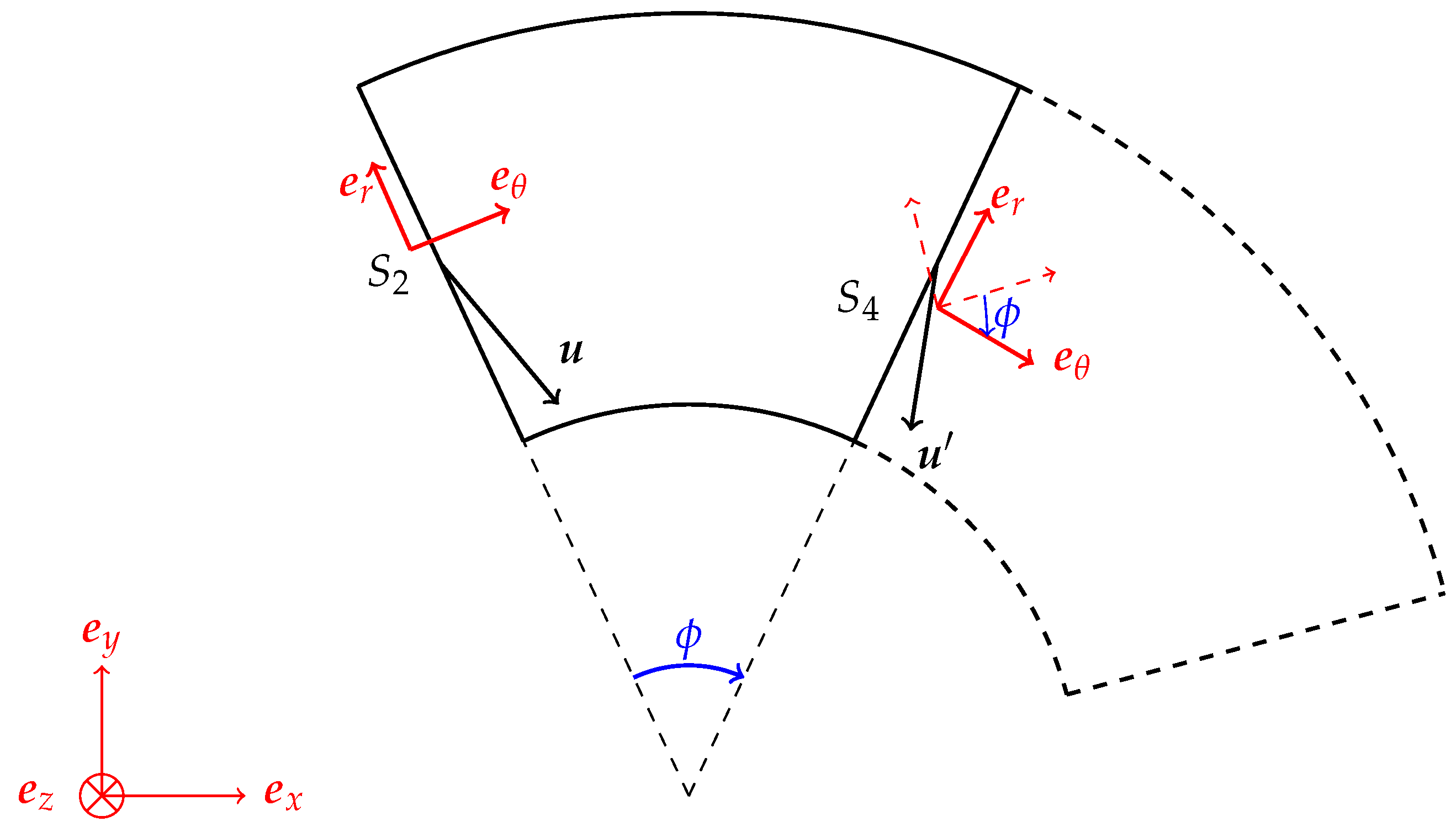
3.2. Implementation Periodic Boundary Conditions
3.3. Mesh Movement
3.3.1. Prescribing the Conformation Tensor
3.4. Time Integration
4. Results
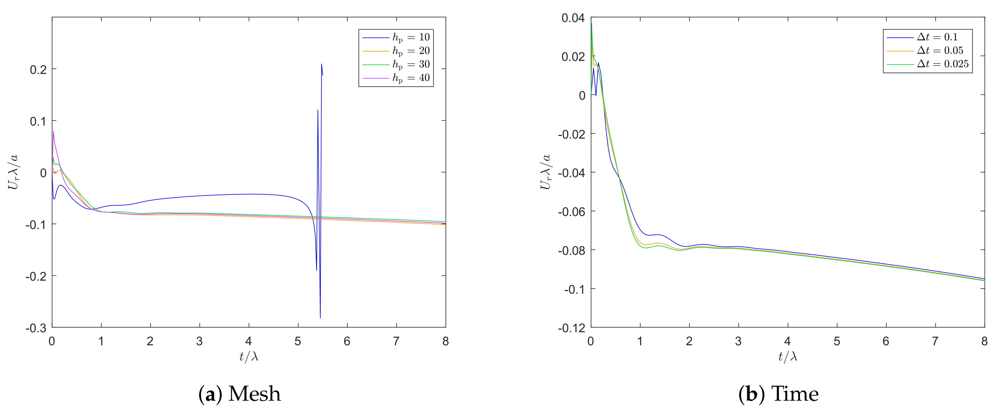
4.1. Convergence
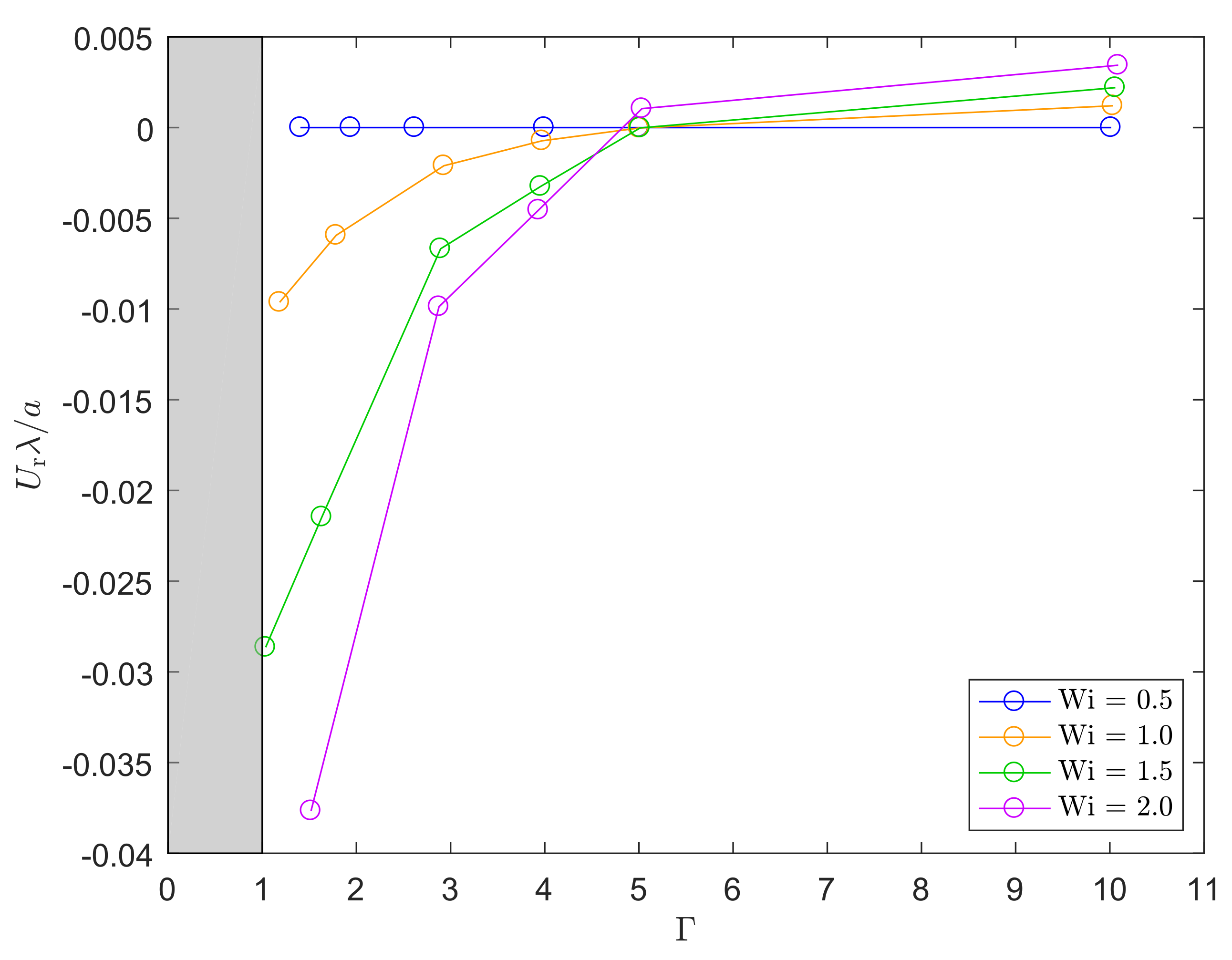
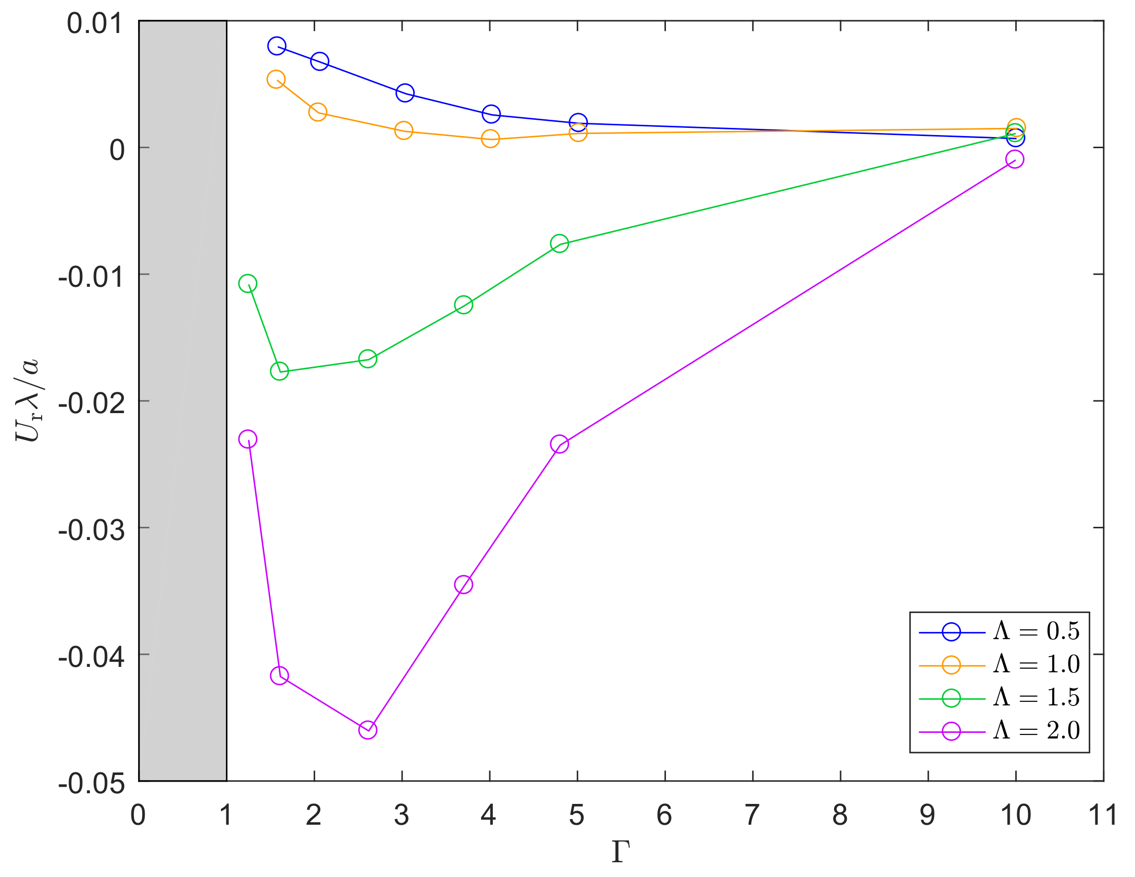
4.2. Migration
4.2.1. Migration for a Falling Particle without Shear in Couette Flow
4.2.2. Migration of a Particle in Couette Flow without Sedimentation
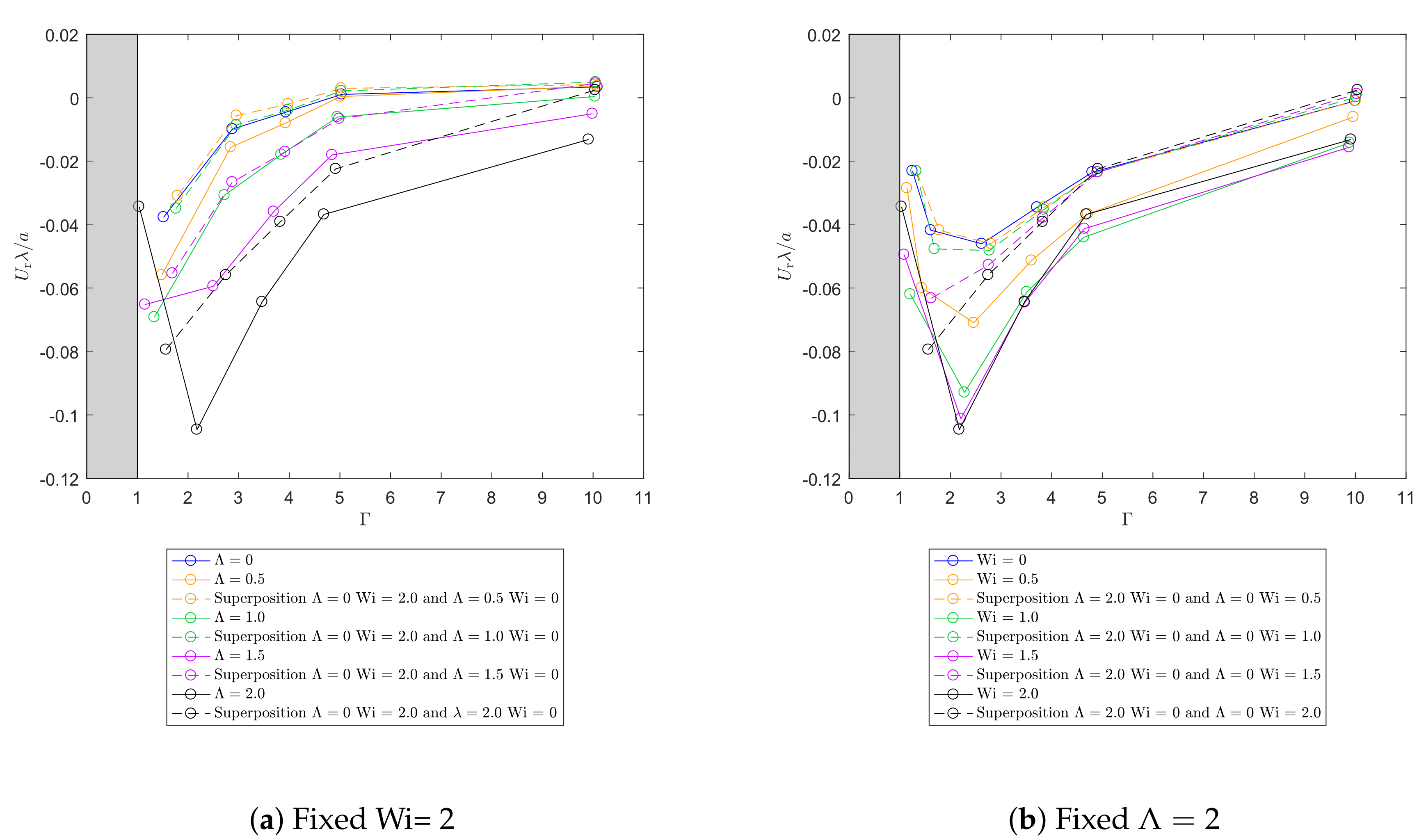
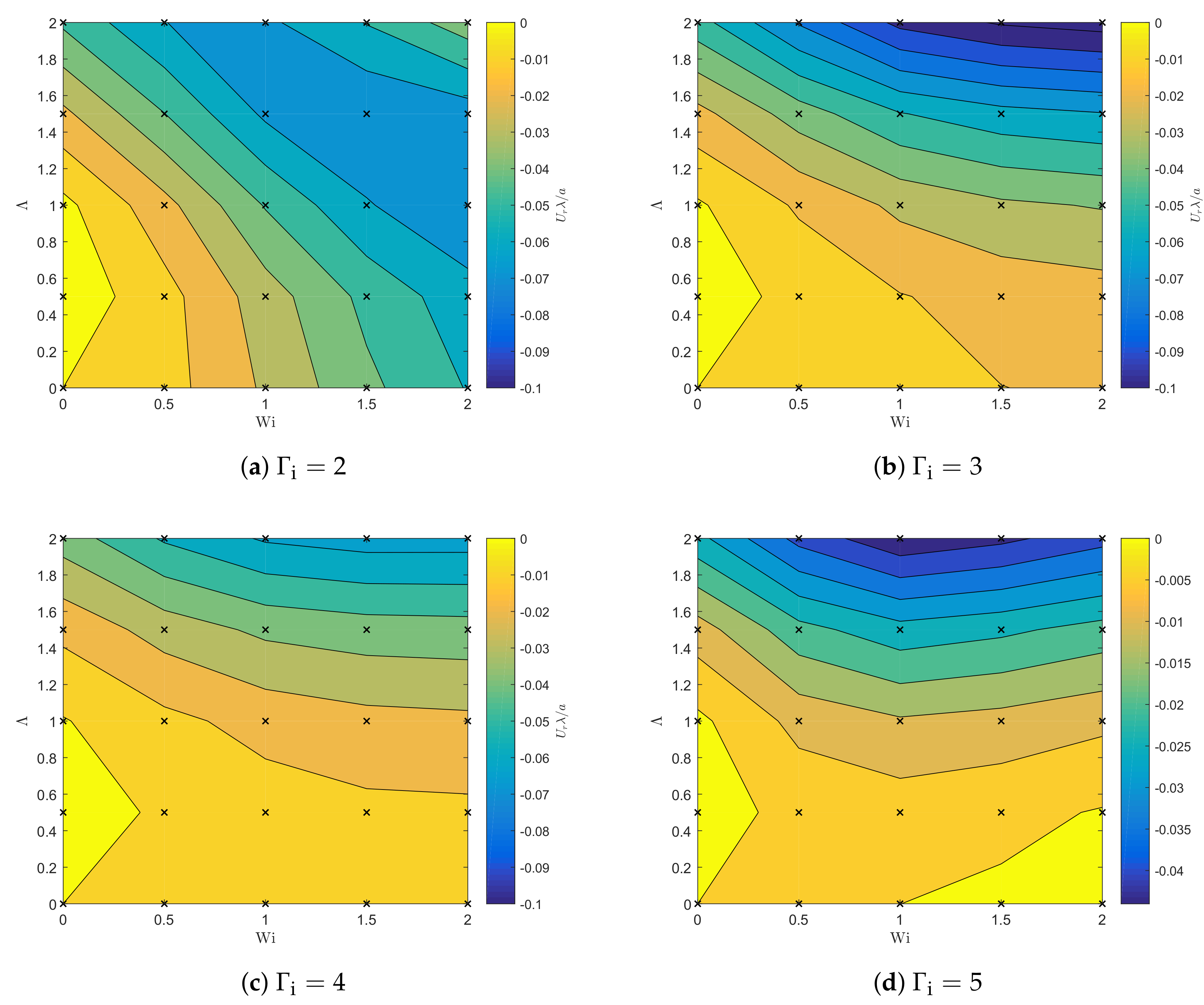
4.2.3. Migration of a Falling Particle in a Shear Flow
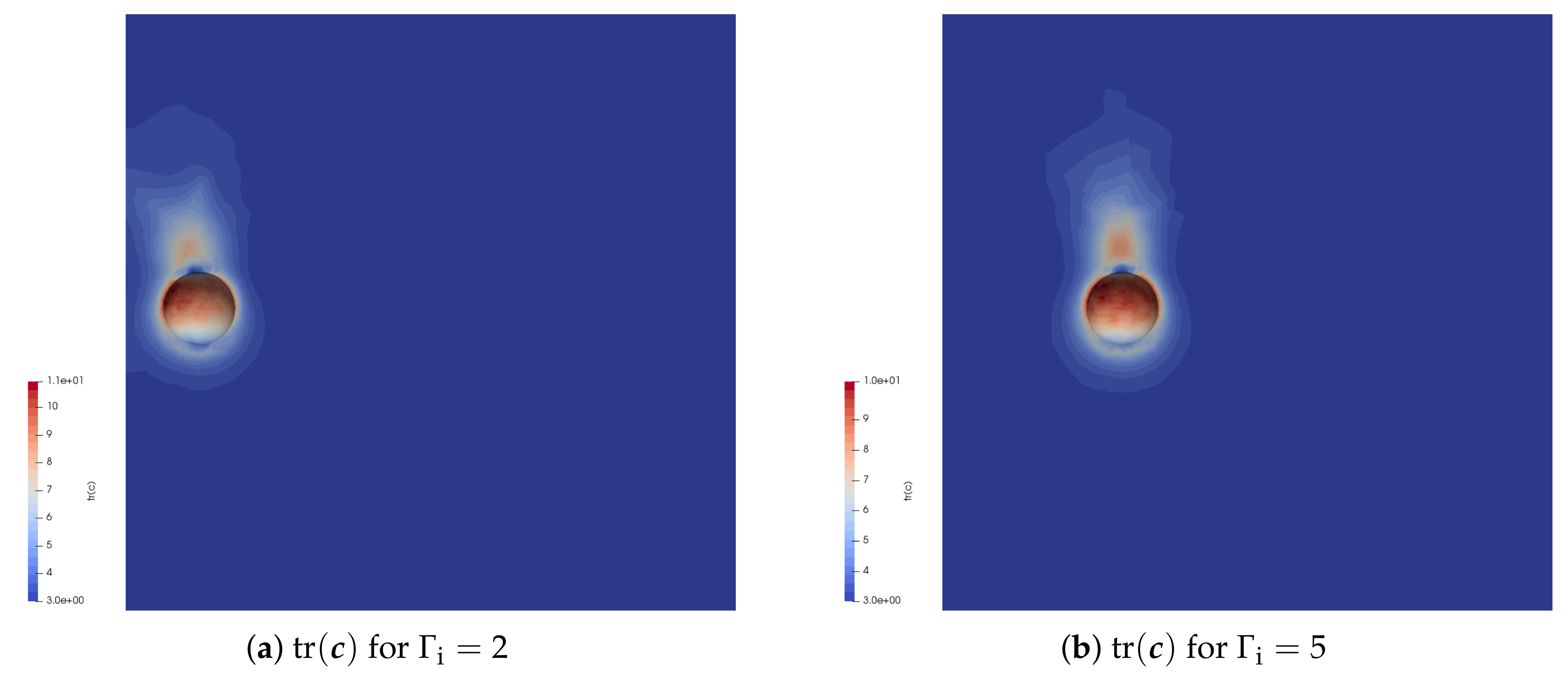
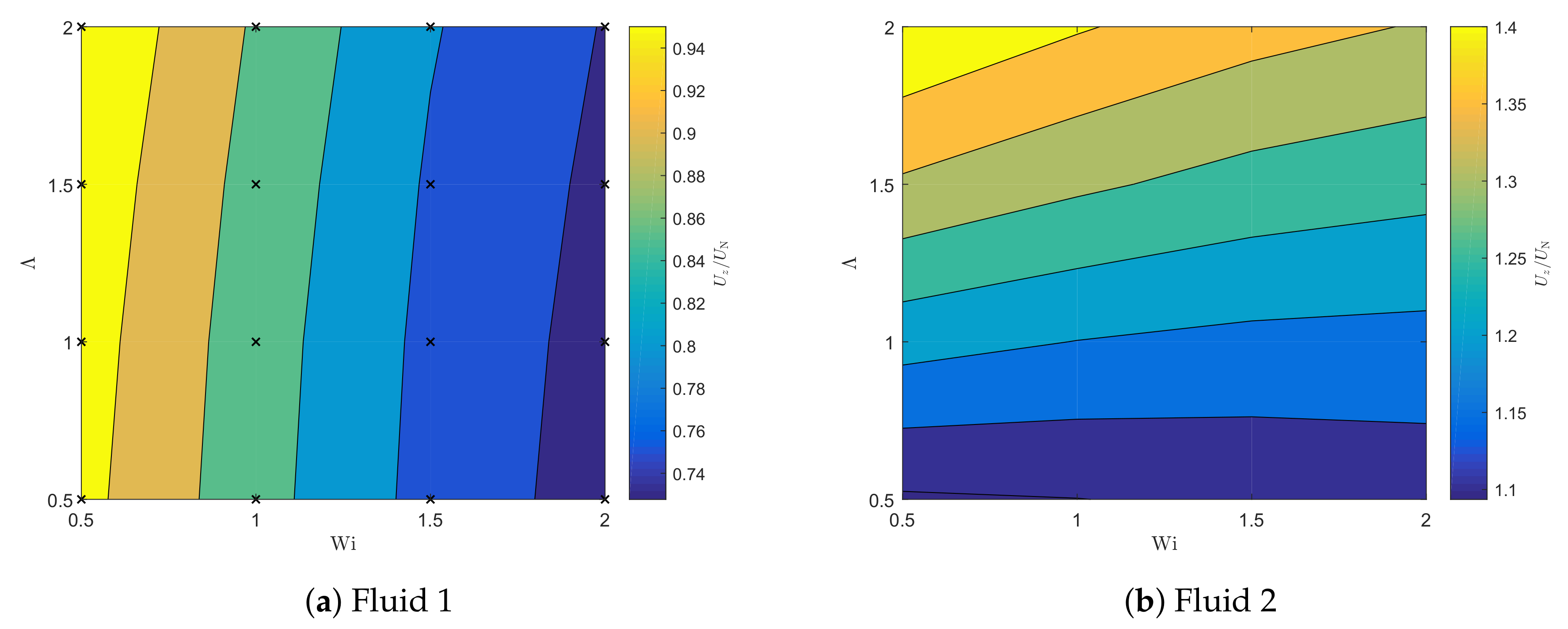
4.3. Sedimentation
5. Conclusions
Author Contributions
Funding
Conflicts of Interest
Appendix A. Periodic Boundary Condition Velocity

Appendix B. Periodic Boundary Condition Conformation Tensor
Appendix B.1. Tensor Rotation
Appendix B.2. Conformation Tensor
References
- Kim, Y.; Yoo, J. Three-dimensional focusing of red blood cells in microchannel flows for bio-sensing applications. Biosens. Bioelectron. 2009, 24, 3677–3682. [Google Scholar] [CrossRef] [PubMed]
- Economides, M.; Nolte, K. Reservoir Stimulation; Prentice Hall: Hoboken, NJ, USA, 1989. [Google Scholar]
- Singh, P.; Joseph, D. Sedimentation of a sphere near a vertical wall in an Oldroyd-B fluid. J. Non-Newton. Fluid Mech. 2000, 94, 179–203. [Google Scholar] [CrossRef]
- D’Avino, G.; Tuccillo, T.; Maffettone, P.; Greco, F.; Hulsen, M. Numerical simulations of particle migration in a viscoelastic fluid subjected to shear flow. Comput. Fluids 2010, 39, 709–721. [Google Scholar] [CrossRef]
- D’Avino, G.; Snijkers, F.; Pasquino, R.; Hulsen, M.; Greco, F.; Maffettone, P.; Vermant, J. Migration of a sphere suspended in viscoelastic liquids in Couette flow: Experiments and simulations. Rheol. Acta 2012, 51, 215–234. [Google Scholar] [CrossRef]
- Chilcott, M.; Rallison, J. Creeping flow of dilute polymer solutions past cylinders and spheres. J. Non-Newton. Fluid Mech. 1988, 29, 381–432. [Google Scholar] [CrossRef]
- Harlen, O.; Rallison, J.; Chilcott, M. High-Deborah-number flows of dilute polymer solutions. J. Non-Newton. Fluid Mech. 1990, 34, 319–349. [Google Scholar] [CrossRef]
- Arigo, M.; Rajagopalan, D.; Shapley, N.; McKinley, G. The sedimentation of a sphere through an elastic fluid. Part 1. Steady motion. J. Non-Newton. Fluid Mech. 1995, 60, 225–27. [Google Scholar] [CrossRef]
- D’Avino, G.; Maffettone, P. Particle dynamics in viscoelastic liquids. J. Non-Newton. Fluid Mech. 2015, 215, 80–104. [Google Scholar] [CrossRef]
- Van den Brule, B.; Gheissary, G. Effects of fluid elasticity on the static and dynamic settling of a spherical particle. J. Non-Newton. Fluid Mech. 1993, 49, 123–132. [Google Scholar] [CrossRef]
- Padhy, S.; Rodriguez, M.; Shaqfeh, E.; Iaccarino, G.; Morris, J.; Tonmakayakul, N. The effect of shear thinning and walls on the sedimentation of a sphere in an elastic fluid under orthogonal shear. J. Non-Newton. Fluid Mech. 2013, 201, 120–129. [Google Scholar] [CrossRef]
- Padhy, S.; Shaqfeh, E.; Iaccarino, G.; Morris, J.; Tonmakayakul, N. Simulations of a sphere sedimenting in a viscoelastic fluid with cross shear flow. J. Non-Newton. Fluid Mech. 2013, 197, 48–60. [Google Scholar] [CrossRef]
- Murch, W.; Krishnan, S.; Shaqfeh, E.; Iaccarino, G. Growth of viscoelastic wings and the reduction of particle mobility in a viscoelastic shear flow. Phys. Rev. Fluids 2017, 2, 103302. [Google Scholar] [CrossRef]
- Giesekus, H. A simple constitutive equation for polymer fluids based on the concept of deformation-dependent tensorial mobility. J. Non-Newton. Fluid Mech. 1982, 11, 69–109. [Google Scholar] [CrossRef]
- Hu, H.; Patankar, N.; Zhu, M. Direct numerical simulations of fluid-solid systems using the arbitrary Lagrangian-Eulerian technique. J. Comput. Phys. 2001, 169, 427–462. [Google Scholar] [CrossRef]
- Hulsen, M.; Fattal, R.; Kupferman, R. Flow of viscoelastic fluids past a cylinder at high Weissenberg number: Stabilized simulations using matrix logarithms. J. Non-Newton. Fluid Mech. 2005, 127, 27–39. [Google Scholar] [CrossRef]
- Bogaerds, A.; Grillet, A.; Peters, G.; Baaijens, F. Stability analysis of polymer shear flows using the extended pom-pom constitutive equations. J. Non-Newton. Fluid Mech. 2002, 108, 187–208. [Google Scholar] [CrossRef]
- Glowinski, R.; Pan, T.; Hesla, T.; Joseph, D. A distributed Lagrange multiplier/fictitious domain method for particulate flows. Int. J. Multiph. Flow 1999, 25, 755–794. [Google Scholar] [CrossRef]
- Geuzaine, C.; Remacle, J. Gmsh: A 3D finite element mesh generator with built-in pre- and post-processing facilities. Int. J. Numer. Methods Eng. 2009, 79, 1–24. [Google Scholar] [CrossRef]
- Jaensson, N.; Hulsen, M.; Anderson, P. Stokes-Cahn-Hilliard formulations and simulations of two-phase flows with suspended rigid particles. Comput. Fluids 2015, 111, 1–17. [Google Scholar] [CrossRef]
- Van der Zanden, J.; Hulsen, M. Mathematical and physical requirements for successful computations with viscoelastic fluid models. J. Non-Newton. Fluid Mech. 1988, 29, 93–117. [Google Scholar] [CrossRef]
- Renardy, M. Inflow boundary conditions for steady flows of viscoelastic fluids with differential constitutive laws. J. Non-Newton. Fluid Mech. 1988, 18, 445–454. [Google Scholar]
- D’Avino, G.; Hulsen, M. Decoupled second-order transient schemes for the flow of viscoelastic fluids without a viscous solvent contribution. J. Non-Newton. Fluid Mech. 2010, 165, 1602–1612. [Google Scholar] [CrossRef]
- Snijkers, F.; D’Avino, G.; Maffettone, P.; Greco, F.; Hulsen, M.; Vermant, J. Effect of viscoelasticity on the rotation of a sphere in shear flow. J. Non-Newton. Fluid Mech. 2011, 166, 363–372. [Google Scholar] [CrossRef]


| Non-Linear Parameter | ||
|---|---|---|
| Fluid 1 | 0.5 | 0.01 |
| Fluid 2 | 0.35 | 0.2 |
© 2019 by the authors. Licensee MDPI, Basel, Switzerland. This article is an open access article distributed under the terms and conditions of the Creative Commons Attribution (CC BY) license (http://creativecommons.org/licenses/by/4.0/).
Share and Cite
Spanjaards, M.M.A.; Jaensson, N.O.; Hulsen, M.A.; Anderson, P.D. A Numerical Study of Particle Migration and Sedimentation in Viscoelastic Couette Flow. Fluids 2019, 4, 25. https://doi.org/10.3390/fluids4010025
Spanjaards MMA, Jaensson NO, Hulsen MA, Anderson PD. A Numerical Study of Particle Migration and Sedimentation in Viscoelastic Couette Flow. Fluids. 2019; 4(1):25. https://doi.org/10.3390/fluids4010025
Chicago/Turabian StyleSpanjaards, Michelle M. A., Nick O. Jaensson, Martien A. Hulsen, and Patrick D. Anderson. 2019. "A Numerical Study of Particle Migration and Sedimentation in Viscoelastic Couette Flow" Fluids 4, no. 1: 25. https://doi.org/10.3390/fluids4010025
APA StyleSpanjaards, M. M. A., Jaensson, N. O., Hulsen, M. A., & Anderson, P. D. (2019). A Numerical Study of Particle Migration and Sedimentation in Viscoelastic Couette Flow. Fluids, 4(1), 25. https://doi.org/10.3390/fluids4010025