Assessment of Turbulence Models in a Hypersonic Cold-Wall Turbulent Boundary Layer


Department of Mechanical and Aerospace Engineering, Missouri University of Science and Technology, Rolla, MO 65409, USA
*
Author to whom correspondence should be addressed.
Fluids 2019, 4(1), 37; https://doi.org/10.3390/fluids4010037
Submission received: 31 January 2019
/
Revised: 11 February 2019
/
Accepted: 17 February 2019
/
Published: 26 February 2019
(This article belongs to the Special Issue Turbulence and Transitional Modeling of Aerodynamic Flows)
Abstract
:In this study, the ability of standard one- or two-equation turbulence models to predict mean and turbulence profiles, the Reynolds stress, and the turbulent heat flux in hypersonic cold-wall boundary-layer applications is investigated. The turbulence models under investigation include the one-equation model of Spalart–Allmaras, the baseline model by Menter, as well as the shear-stress transport model by Menter. Reynolds-Averaged Navier-Stokes (RANS) simulations with the different turbulence models are conducted for a flat-plate, zero-pressure-gradient turbulent boundary layer with a nominal free-stream Mach number of 8 and wall-to-recovery temperature ratio of , and the RANS results are compared with those of direct numerical simulations (DNS) under similar conditions. The study shows that the selected eddy-viscosity turbulence models, in combination with a constant Prandtl number model for turbulent heat flux, give good predictions of the skin friction, wall heat flux, and boundary-layer mean profiles. The Boussinesq assumption leads to essentially correct predictions of the Reynolds shear stress, but gives wrong predictions of the Reynolds normal stresses. The constant Prandtl number model gives an adequate prediction of the normal turbulent heat flux, while it fails to predict transverse turbulent heat fluxes. The discrepancy in model predictions among the three eddy-viscosity models under investigation is small.
1. Introduction
Accurate modeling of cold-wall hypersonic turbulent boundary layers (TBLs) is critically important to the prediction of the surface heat flux, and hence, to the design of thermal protection systems for hypersonic vehicles. Yet, the existing literature on hypersonic TBLs is rather limited, whether in regard to measurements, modeling, or numerical simulations [1,2,3,4,5,6,7,8,9,10]. Reynolds-Averaged Navier-Stokes (RANS) turbulence models have been widely used for simulating hypersonic turbulent boundary layers, without any specific considerations regarding the high-Mach-number effects. Standard one- or two-equation turbulence models, such as the Spalart-Allmaras (SA) Model and the Menter’s Shear Stress Transport (SST) Model, have been developed largely based on studies of subsonic or moderately supersonic flows with adiabatic walls. Thus, careful assessment of model performance is necessary before such models can be extended to applications in the hypersonic, cold-wall regime. Despite many previous efforts to assess existing models for hypersonic applications (see, for example, the review by Roy and Blottner [2] and references therein), continued research to develop better physics-based compressible turbulence modeling is clearly needed for flows in the hypersonic regime, starting with attached boundary layers.
One of the primary objectives of this paper is to assess some commonly used eddy-viscosity turbulence models (Spalart–Allmaras, Menter’s Baseline, and SST models) under hypersonic, cold-wall conditions, using a newly developed direct numerical simulation (DNS) database of supersonic and hypersonic turbulent boundary layers [10]. The flow configuration we focus on is a spatially-developing, zero-pressure-gradient, flat-plate turbulent boundary layer at, nominally, Mach 8, with a wall-to-recovery temperature ratio of . The current study contains detailed comparisons of mean and turbulence profiles against the DNS that are complementary to the few model evaluation efforts in the literature under high-Mach-number, cold-wall conditions that were limited to comparing wall quantities (skin friction, Stanton number, and wall pressure) with experimental data and empirical correlations [4,11].
Another objective of the current study is to use high-fidelity DNS to assess compressibility corrections for hypersonic, cold-wall turbulent boundary layers. Rumsey [11] provided a recent review of the most common classes of compressibility correction for the form of two-equation models. He also assessed the influence of compressibility corrections on turbulent skin friction in hypersonic boundary layers. The current study will extend such an assessment to mean velocity and temperature fields.
2. Underlying Methodology
2.1. DNS Simulation of Hypersonic Turbulent Boundary Layers
To provide benchmark data for testing RANS models, the DNS of hypersonic turbulent boundary layers was conducted over a flat plate. The DNS simulation with flat plate is referred to as Case “DNS-FlatPlate”. Targeted flow conditions in the free stream for Case DNS-FlatPlate are summarized in Table 1, including the freestream Mach number , velocity , density , and temperature . The wall is assumed to be isothermal, with a wall temperature of K. The corresponding wall-to-recovery temperature ratio is , with the recovery temperature estimated as based on a recovery factor of , and is the specific heat ratio. Case DNS-FlatPlate corresponds to the DNS reported (Case M8Tw048) in a previous paper by our group [10], in which the underlying methodology and validation are presented in detail. The DNS case falls within the perfect gas regime. The working fluid is nitrogen, and its viscosity was calculated by using the Keyes law [12]. A constant molecular Prandtl number of was used for the DNS case.
To perform DNS of turbulent boundary layers, the full three-dimensional compressible Navier-Stokes equations in conservation form are solved numerically in curvilinear Cartesian coordinates. The boundary layer is simulated in a rectangular box over a flat plate with spanwise periodic boundary conditions and a modified rescaling/recycling method for inflow turbulence generation [13]. The inviscid fluxes of the governing equations are computed using a seventh-order weighted essentially non-oscillatory (WENO) scheme. Compared with the original finite-difference WENO introduced by Jiang and Shu [14], the present scheme is optimized by means of limiters [15,16] to reduce the numerical dissipation. The viscous fluxes are discretized using a fourth-order central difference scheme, and time integration is performed using a third-order low-storage Runge-Kutta scheme [17]. The simulation involves a single domain with a long streamwise box, as illustrated in Figure 1. A detailed description of the problem formulation, the numerical scheme, and the initial and boundary conditions can be found in References [13,18,19,20,21,22]. The validity of the numerical methods and procedures have been established in multiple previous publications [10,18,21,22].
2.2. RANS Simulation of Hypersonic Turbulent Boundary Layers
RANS simulations of high-speed turbulent boundary layers were conducted, with the flow conditions and thermodynamic equation of state matching that of the DNS case listed in Table 1. In RANS, ANSYS Fluent (Version 18.0, ANSYS, Inc., Canonsburg, PA, USA) [23] is used to solve the compressible Favre-averaged Navier-Stokes equations [24], which can be written as:
where , , and . Throughout the paper, standard (Reynolds) averages are denoted by an overbar, , while density-weighted (Favre) averages are denoted by a tilde, ; fluctuations around standard and Favre averages are denoted by single and double primes, as with and , respectively.
In the one- or two-equation turbulence models under investigation, the Reynolds stress term was modeled by the Boussinesq approximation:
where is the mean velocity strain, and is the eddy viscosity obtained by a turbulence model to be discussed later, and k is the turbulent kinetic energy. The turbulent heat flux term was modeled based on the Reynolds analogy as:
where the turbulent Prandtl number is assumed to be a constant of . The terms associated with molecular diffusion and turbulent transport in the Farve-averaged energy equation are neglected in the current study [25].
In the current study, two-dimensional planar RANS were conducted with a few representative turbulence models, selected among those in widespread use in the aerospace industry. The models chosen are the one-equation model of Spalart–Allmaras [26], the baseline model by Menter [27], and the shear-stress transport model by Menter [27]. Unless otherwise mentioned, the “standard” form” (i.e., the original published form) of the model equations was used, with the detailed information on the model formula and coefficients listed in Reference [28,29,30]. Similar to the DNS, ideal gas relations were used in the RANS simulations with nitrogen as the working fluid, and the Keyes law [12] was used for dynamic viscosity.
As far as the compressibility correction is concerned, a complete investigation of all forms of compressibility correction in the literature was not among the goals of this work. We chose to focus on the Wilcox form of compressibility correction [31], which was specifically developed for hypersonic applications. In Wilcox compressibility correction, correction is achieved through the modification of the coefficient in the destruction term [25,31]. For instance, the modified coefficient of the destruction term in the equation is:
where and is the original coefficient. The compressibility function is obtained as:
where is the turbulent Mach number, , and is the speed of sound.
Figure 2 shows a schematic of the computational domain for Case RANS-FlatPlate along with the boundary conditions. The streamwise (x) and wall-normal (y) domain sizes are , where the reference length mm is the boundary-layer thickness at the center of the domain. Here, the boundary-layer thickness is defined as the wall-normal height at which the streamwise velocity reaches of the freestream velocity. Throughout the paper, the velocity components in the streamwise, wall-normal, and spanwise (z) directions are u, v, and w, respectively. A mesh of grid is used in streamwise and wall-normal directions, respectively. A uniform grid distribution is used in the streamwise direction with a resolution of . In the wall-normal direction, a geometric distribution with a stretch ratio of less than 1.05 is used to cluster meshes near the wall. The wall-normal grid resolution is at the wall and near the boundary layer edge. The grid resolutions are normalized by the viscous length at , where the turbulence statistics are reported, and the value of is listed in Table 2. To monitor grid convergence, a grid study was conducted using the SST model on the baseline grid (), along with two successively coarser grids for which every other grid point was removed in each coordinate direction ( and ) and one refined grid () with two times higher grid resolution in the streamwise direction. Results are shown in Figure 3, where is the wall skin friction coefficient with the wall shear stress, and is the wall heat flux coefficient with the wall heat flux and the heat capacity at constant pressure. Over most of the plate, the four grids yielded very close results. The difference in between the baseline grid and the finest grid is less than at .
3. Results
In this section, the RANS of hypersonic turbulent boundary layers were conducted with different turbulence models. The performance of each model is assessed by comparing RANS against DNS.
Figure 4 shows comparisons of the wall skin friction coefficient and wall heat transfer coefficient among DNS, RANS, and the empirical correlations of van Driest [32] and Spalding–Chi [33]. In general, the RANS cases give good predictions of surface skin friction and heat flux, especially when the SST model is used. For all RANS cases, the predictions of and lie within of those of the DNS. Consistent with previous findings [11,34], the van Driest correlation gives significantly better predictions of skin friction and wall heat flux coefficients than the Spalding–Chi correlation.
Additionally, boundary-layer integral and wall parameters and profiles predicted by DNS and RANS were compared with a common friction Reynolds number of . Table 2 summarizes the boundary-layer parameters at the selected location for both cases, including the momentum thickness , shape factor (where is the displacement thickness), boundary layer thickness , friction velocity , viscous length , wall skin friction coefficient , Reynolds analogy factor (where is the wall heat transfer coefficient), dimensionless wall heat transfer rate , and different definitions of the Reynolds number, namely , , and . Figure 5 further shows a comparison in the mean boundary-layer profiles between RANS and DNS. The selected eddy-viscosity turbulence models, in combination with a constant Prandtl number model for turbulent heat flux, give good predictions of boundary-layer parameters and mean profiles. The discrepancy in model predictions among the different models is small.
In terms of turbulence quantities, Figure 6 compares the Reynolds stresses between RANS and DNS cases. In RANS, the Reynolds stresses were derived using turbulent viscosity and the mean velocity gradient, according to the Boussinesq assumption (Equation (4)). Good comparison was achieved for the Reynolds shear stress . However, the Reynolds streamwise stress was significantly underpredicted by RANS. Figure 7 shows that the turbulent normal heat flux , calculated according to the Reynolds analogy assumption (Equation (5)), compares well with the DNS. The turbulent transverse heat flux (), however, is not properly predicted by RANS.
Lastly, the Wilcox form of compressibility correction [31] is investigated. Figure 8 plots the predictions of boundary-layer mean profiles by Menter’s SST model with and without compressibility correction. The comparison of RANS with the DNS shows that the Wilcox form of compressibility correction causes only a small change in the mean boundary-layer profiles, and no improvement is shown over the standard SST model for the current flow. A similar trend is found when the compressibility correction is used with the BSL model.
4. Conclusions
In this article, the performance of three commonly used eddy-viscosity models (Spalart-Allmaras, SST, BSL) was assessed under hypersonic cold-wall conditions. The model evaluation effort focuses on comparing mean and turbulence profiles with DNS for a spatially-developing, zero-pressure-gradient, flat-plate turbulent boundary layer at nominally Mach 8 with . The study shows that the selected eddy-viscosity models provide good predictions for turbulent skin friction, wall heat flux, and the mean mass flux and temperature profiles. The use of Boussinesq and Reynolds analogy assumptions also provides acceptable predictions to the Reynolds shear stress, , and the turbulent normal heat flux, . Such assumptions, however, lead to wrong predictions of Reynolds normal stresses () and the turbulent transverse heat flux (). The Wilcox form of compressibility correction was found to cause only a small change in the mean boundary-layer profiles, and no improvement was shown over the standard model without correction.
Author Contributions
Conceptualization, J.H. and L.D.; methodology, J.H.; formal analysis, J.H. and J.-V.B.; investigation, J.H. and J.-V.B.; resources, L.D.; data curation, J.H. and J.-V.B.; writing—original draft preparation, J.H. and L.D.; writing—review and editing, L.D.; visualization, J.H.; supervision, L.D.; project administration, L.D.; funding acquisition, L.D.
Funding
This research received no external funding.
Conflicts of Interest
The authors declare no conflict of interest.
References
- Fernholz, H.H.; Finley, P.J. A critical Commentary on Mean Flow Data for Two-Dimensional Compressible Boundary Layers; No. AGARD-AG-253; Advisory Group for Aerospace Research and Development: Neuilly-sur-Seine, France, 1980. [Google Scholar]
- Roy, C.J.; Blottner, F.G. Review and Assessment of Turbulence Models for Hypersonic Flows. Prog. Aerosp. Sci. 2006, 42, 469–530. [Google Scholar] [CrossRef]
- Smits, A.J.; Dussauge, J.P. Turbulent Shear Layers in Supersonic Flow, 2nd ed.; American Institute of Physics: Melville, NY, USA, 2006. [Google Scholar]
- Holden, M.S.; Wadhams, T.P.; MacLean, M. Measurements in Regions of Shock Wave/Turbulent Boundary Layer Interaction from Mach 4 to 10 at Flight Duplicated Velocities to Evaluate and Improve the Models of Turbulence in CFD Codes. In Proceedings of the 22nd AIAA Computational Fluid Dynamics Conference, Atlanta, GA, USA, 16–20 June 2014. [Google Scholar]
- Tichenor, N.R.; Humble, R.A.; Bowersox, R.D.W. Response of a hypersonic turbulent boundary layer to favourable pressure gradients. J. Fluid Mech. 2013, 722, 187–213. [Google Scholar] [CrossRef]
- Flaherty, W.; Austin, J.M. Scaling of heat transfer augmentation due to mechanical distortions in hypervelocity boundary layers. Phys. Fluids 2013, 25, 106106. [Google Scholar] [CrossRef] [Green Version]
- Tichenor, N.R.; Neel, I.; Leidy, A.; Bowersox, R.D. Influence of Streamline Adverse Pressure Gradients on the Structure of a Mach 5 Turbulent Boundary Layer. In Proceedings of the 55th AIAA Aerospace Sciences Meeting, Grapevine, TX, USA, 9–13 January 2017; p. 1697. [Google Scholar]
- Peltier, S.J.; Humble, R.A.; Bowersox, R.D.W. Crosshatch Roughness Distortions on a Hypersonic Turbulent Boundary Layer. Phys. Fluids 2016, 28, 045105. [Google Scholar] [CrossRef]
- Williams, O.J.; Sahoo, D.; Baumgartner, M.L.; Smits, A.J. Experiments on the structure and scaling of hypersonic turbulent boundary layers. J. Fluid Mech. 2018, 834, 237–270. [Google Scholar] [CrossRef]
- Zhang, C.; Duan, L.; Choudhari, M.M. Direct Numerical Simulation Database for Supersonic and Hypersonic Turbulent Boundary Layers. AIAA J. 2018, 56, 4297–4311. [Google Scholar] [CrossRef]
- Rumsey, C.L. Compressibility Considerations for k-omega Turbulence Models in Hypersonic Boundary- Layer Applications. J. Spacecr. Rockets 2010, 47, 11–20. [Google Scholar] [CrossRef]
- Keyes, F.G. A Summary of Viscosity and Heat-Conduction Data for He, A, H2, O2, CO, CO2, H2O, and Air. Trans. Am. Soc. Mech. Eng. 1951, 73, 589–596. [Google Scholar]
- Duan, L.; Choudhari, M.M.; Wu, M. Numerical Study of Pressure Fluctuations due to a Supersonic Turbulent Boundary Layer. J. Fluid Mech. 2014, 746, 165–192. [Google Scholar] [CrossRef]
- Jiang, G.S.; Shu, C.W. Efficient Implementation of Weighted ENO Schemes. J. Comput. Phys. 1996, 126, 202–228. [Google Scholar] [CrossRef] [Green Version]
- Taylor, E.M.; Wu, M.; Martín, M.P. Optimization of Nonlinear Error Sources for Weighted Non-Oscillatory Methods in Direct Numerical Simulations of Compressible Turbulence. J. Comput. Phys. 2006, 223, 384–397. [Google Scholar] [CrossRef]
- Wu, M.; Martín, M.P. Direct Numerical Simulation of Supersonic Boundary Layer over a Compression Ramp. AIAA J. 2007, 45, 879–889. [Google Scholar] [CrossRef]
- Williamson, J. Low-Storage Runge-Kutta Schemes. J. Comput. Phys. 1980, 35, 48–56. [Google Scholar] [CrossRef]
- Duan, L.; Choudhari, M.M.; Zhang, C. Pressure Fluctuations Induced by a Hypersonic Turbulent Boundary Layer. J. Fluid Mech. 2016, 804, 578–607. [Google Scholar] [CrossRef]
- Huang, J.; Zhang, C.; Duan, L.; Choudhari, M.M. Direct Numerical Simulation of Hypersonic Turbulent Boundary Layers inside an Axisymmetric Nozzle. In Proceedings of the 55th AIAA Aerospace Sciences Meeting, Grapevine, TX, USA, 9–13 January 2017; p. 0067. [Google Scholar]
- Huang, J.; Duan, L.; Choudhari, M.M. Direct Numerical Simulation of Acoustic Noise Generation from the Nozzle Wall of a Hypersonic Wind Tunnel. In Proceedings of the 47th AIAA Fluid Dynamics Conference, Denver, CO, USA, 5–9 June 2017; p. 3631. [Google Scholar]
- Duan, L.; Choudhari, M.M.; Chou, A.; Munoz, F.; Ali, S.R.C.; Radespiel, R.; Schilden, T.; Schröder, W.; Marineau, E.C.; Casper, K.M.; et al. Characterization of Freestream Disturbances in Conventional Hypersonic Wind Tunnels. J. Spacecr. Rockets 2018. [Google Scholar] [CrossRef]
- Duan, L.; Nicholson, G.L.; Huang, J.; Casper, K.M.; Wagnild, R.M.; Bitter, N.P. Direct Numerical Simulation of Nozzle-Wall Pressure Fluctuations in a Mach 8 Wind Tunnel. In Proceedings of the AIAA Scitech 2019 Forum, San Diego, CA, USA, 7–11 January 2019; p. 0874. [Google Scholar]
- ANSYS® Fluent, Release 18.0, Help System, User Guide; ANSYS, Inc.: Canonsburg, PA, USA, 2017.
- Implementing Turbulence Models into the Compressible RANS Equations. Available online: https://turbmodels.larc.nasa.gov/implementrans.html (accessed on 19 January 2019).
- ANSYS® Fluent, Release 18.0, Help System, Theory Guide; ANSYS, Inc.: Canonsburg, PA, USA, 2017.
- Spalart, P.R.; Allmaras, S.R. A One-Equation Turbulence Model for Aerodynamic Flows. Rech. Aerosp. 1994, 1, 5–21. [Google Scholar]
- Menter, F.R. Two-equation eddy-viscosity turbulence models for engineering applications. AIAA J. 1994, 32, 1598–1605. [Google Scholar] [CrossRef] [Green Version]
- The Spalart-Allmaras Turbulence Model. Available online: https://turbmodels.larc.nasa.gov/spalart.html#sa (accessed on 19 January 2019).
- The Menter Baseline Turbulence Model. Available online: https://turbmodels.larc.nasa.gov/bsl.html (accessed on 19 January 2019).
- The Menter Shear Stress Transport Turbulence Model. Available online: https://turbmodels.larc.nasa.gov/sst.html (accessed on 19 January 2019).
- WILCOX, D. Progress in hypersonic turbulence modeling. In Proceedings of the 22nd Fluid Dynamics, Plasma Dynamics and Lasers Conference, Honolulu, HI, USA, 24–26 June 1991; p. 1785. [Google Scholar]
- Von Driest, E.R. Problem of aerodynamic heating. Aeronaut. Eng. Rev. 1956, 15, 26–41. [Google Scholar]
- Spalding, D.; Chi, S. The drag of a compressible turbulent boundary layer on a smooth flat plate with and without heat transfer. J. Fluid Mech. 1964, 18, 117–143. [Google Scholar] [CrossRef]
- Hopkins, E.J.; Inouye, M. An Evaluation of Theories for Predicting Turbulent Skin Friction and Heat Transfer on Flat Plates at Supersonic and Hypersonic Mach Numbers. AIAA J. 1971, 9, 993–1003. [Google Scholar] [CrossRef]
Figure 1.
Computational domain and simulation setup for direct numerical simulation (DNS) of Mach 8 turbulent boundary layers. An instantaneous flowfield is shown, visualized by an isosurface of the density gradient magnitude, corresponding to , colored by the streamwise velocity. mm is the inflow boundary layer thickness.

Figure 2.
Computational domain and simulation setup for Reynolds-Averaged Navier-Stokes (RANS) of a Mach 8 turbulent boundary layer developing spatially over a flat plate, with the start of plate at . Here, mm is the boundary-layer thickness at the center of the domain. The contours of Mach number are shown in the domain.

Figure 3.
(a) Wall skin friction and (b) wall heat flux coefficients grid convergence study using the SST on four successive grid sizes.
Figure 3.
(a) Wall skin friction and (b) wall heat flux coefficients grid convergence study using the SST on four successive grid sizes.

Figure 4.
Comparison of (a) skin friction coefficient and (b) wall heat transfer coefficient among DNS, RANS, and empirical correlations. Error bars represent of the DNS value.
Figure 4.
Comparison of (a) skin friction coefficient and (b) wall heat transfer coefficient among DNS, RANS, and empirical correlations. Error bars represent of the DNS value.
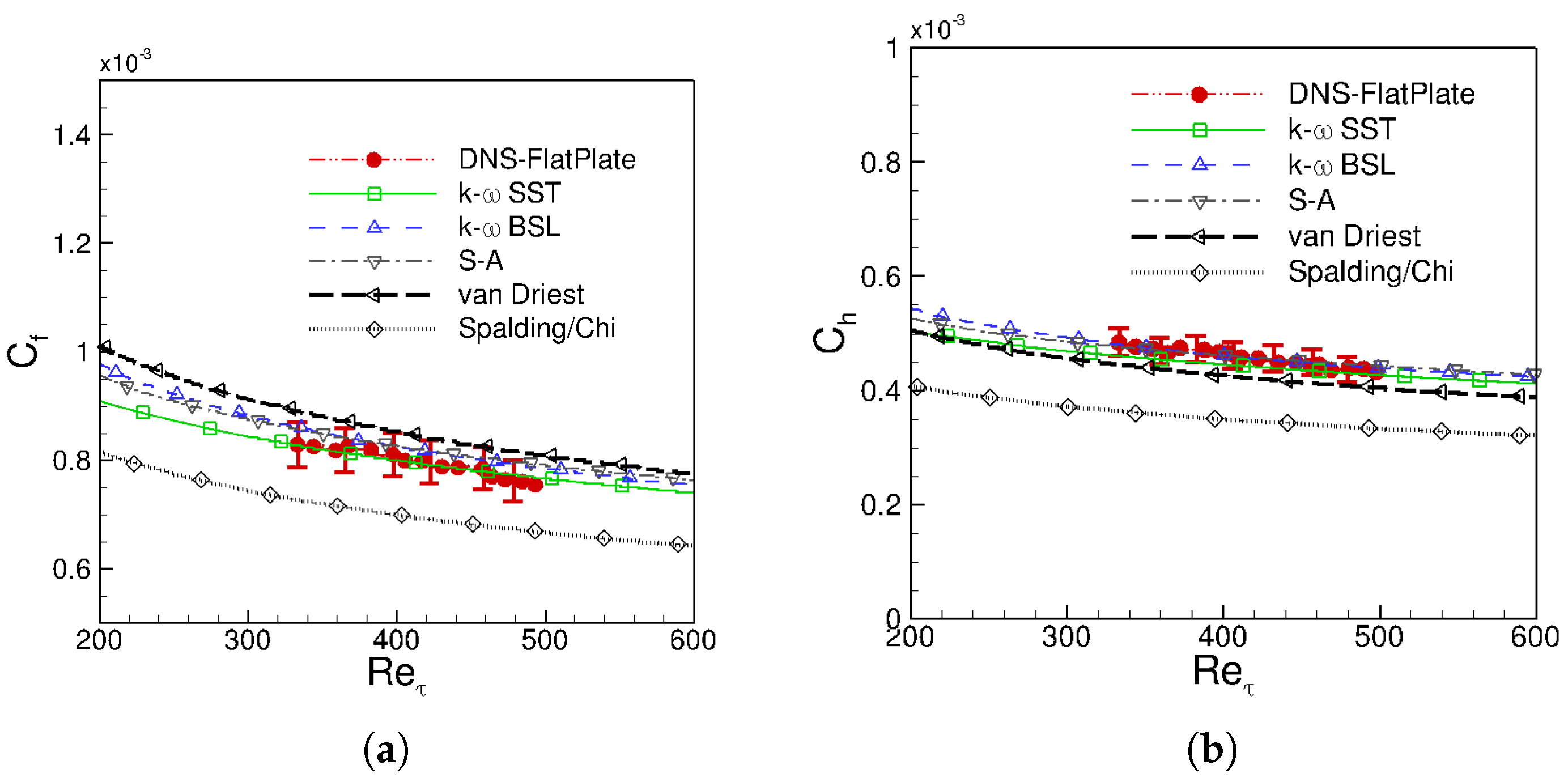
Figure 5.
Comparison of mean boundary-layer profiles at between RANS and DNS. (a) Mean streamwise mass flux ; (b) mean wall-normal mass flux ; (c) mean density ; (d) mean temperature T.
Figure 5.
Comparison of mean boundary-layer profiles at between RANS and DNS. (a) Mean streamwise mass flux ; (b) mean wall-normal mass flux ; (c) mean density ; (d) mean temperature T.

Figure 6.
Comparison of Reynolds stresses at between RANS and DNS. (a) Reynolds streamwise stress ; (b) Reynolds wall-normal stress ; (c) Reynolds spanwise stress ; (d) Reynolds shear stress .
Figure 6.
Comparison of Reynolds stresses at between RANS and DNS. (a) Reynolds streamwise stress ; (b) Reynolds wall-normal stress ; (c) Reynolds spanwise stress ; (d) Reynolds shear stress .

Figure 7.
Comparison of turbulent heat fluxes at between RANS and DNS. (a) turbulent transverse heat flux ; (b) turbulent normal heat flux .
Figure 7.
Comparison of turbulent heat fluxes at between RANS and DNS. (a) turbulent transverse heat flux ; (b) turbulent normal heat flux .

Figure 8.
Comparison of mean boundary-layer profiles at between DNS and RANS using SST with and without compressibility corrections. (a) Mean mass flux ; (b) mean wall-normal mass flux ; (c) mean density ; (d) mean temperature T.
Figure 8.
Comparison of mean boundary-layer profiles at between DNS and RANS using SST with and without compressibility corrections. (a) Mean mass flux ; (b) mean wall-normal mass flux ; (c) mean density ; (d) mean temperature T.


Table 1.
Freestream and wall-temperature conditions for the direct numerical simulation (DNS) of a Mach 8 turbulent boundary layer.
Table 1.
Freestream and wall-temperature conditions for the direct numerical simulation (DNS) of a Mach 8 turbulent boundary layer.
| Case | (m/s) | (kg/m) | (K) | (K) | ||
|---|---|---|---|---|---|---|
| DNS-FlatPlate | 7.87 | 1155.1 | 0.026 | 51.8 | 298.0 | 0.48 |
Table 2.
Comparison of boundary-layer parameters between RANS and DNS.
| Case | (mm) | H | (mm) | (m) | (m/s) | RA | |||||
|---|---|---|---|---|---|---|---|---|---|---|---|
| DNS-FlatPlate | 8748 | 479 | 1930 | 1.22 | 16.2 | 35.3 | 54.1 | 0.76 | 1.14 | 0.06 | |
| SST | 8856 | 482 | 1895 | 1.08 | 19.1 | 32.6 | 67.7 | 53.9 | 0.77 | 1.11 | 0.06 |
| BSL | 9295 | 498 | 1984 | 1.13 | 19.2 | 33.4 | 67.0 | 54.3 | 0.79 | 1.12 | 0.06 |
| S-A | 8440 | 479 | 1821 | 1.04 | 18.9 | 31.8 | 66.5 | 54.8 | 0.80 | 1.12 | 0.06 |
© 2019 by the authors. Licensee MDPI, Basel, Switzerland. This article is an open access article distributed under the terms and conditions of the Creative Commons Attribution (CC BY) license (http://creativecommons.org/licenses/by/4.0/).
Share and Cite
MDPI and ACS Style
Huang, J.; Bretzke, J.-V.; Duan, L. Assessment of Turbulence Models in a Hypersonic Cold-Wall Turbulent Boundary Layer. Fluids 2019, 4, 37. https://doi.org/10.3390/fluids4010037
AMA Style
Huang J, Bretzke J-V, Duan L. Assessment of Turbulence Models in a Hypersonic Cold-Wall Turbulent Boundary Layer. Fluids. 2019; 4(1):37. https://doi.org/10.3390/fluids4010037
Chicago/Turabian StyleHuang, Junji, Jorge-Valentino Bretzke, and Lian Duan. 2019. "Assessment of Turbulence Models in a Hypersonic Cold-Wall Turbulent Boundary Layer" Fluids 4, no. 1: 37. https://doi.org/10.3390/fluids4010037