Numerical Investigation of Air-Side Heat Transfer and Pressure Drop Characteristics of a New Triangular Finned Microchannel Evaporator with Water Drainage Slits


Abstract
:
1. Introduction
2. Method
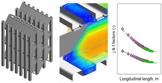
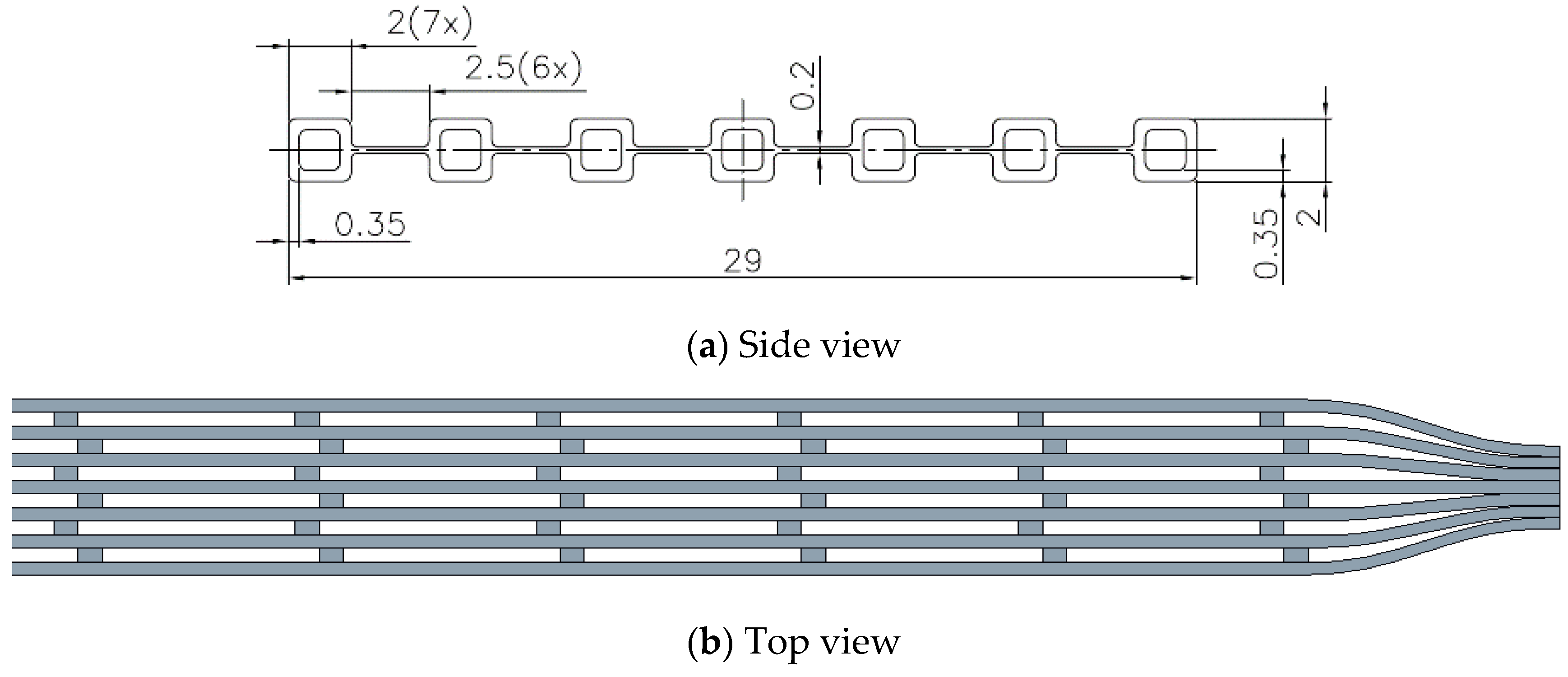
2.1. Geometry of the Microchannel Evaporator
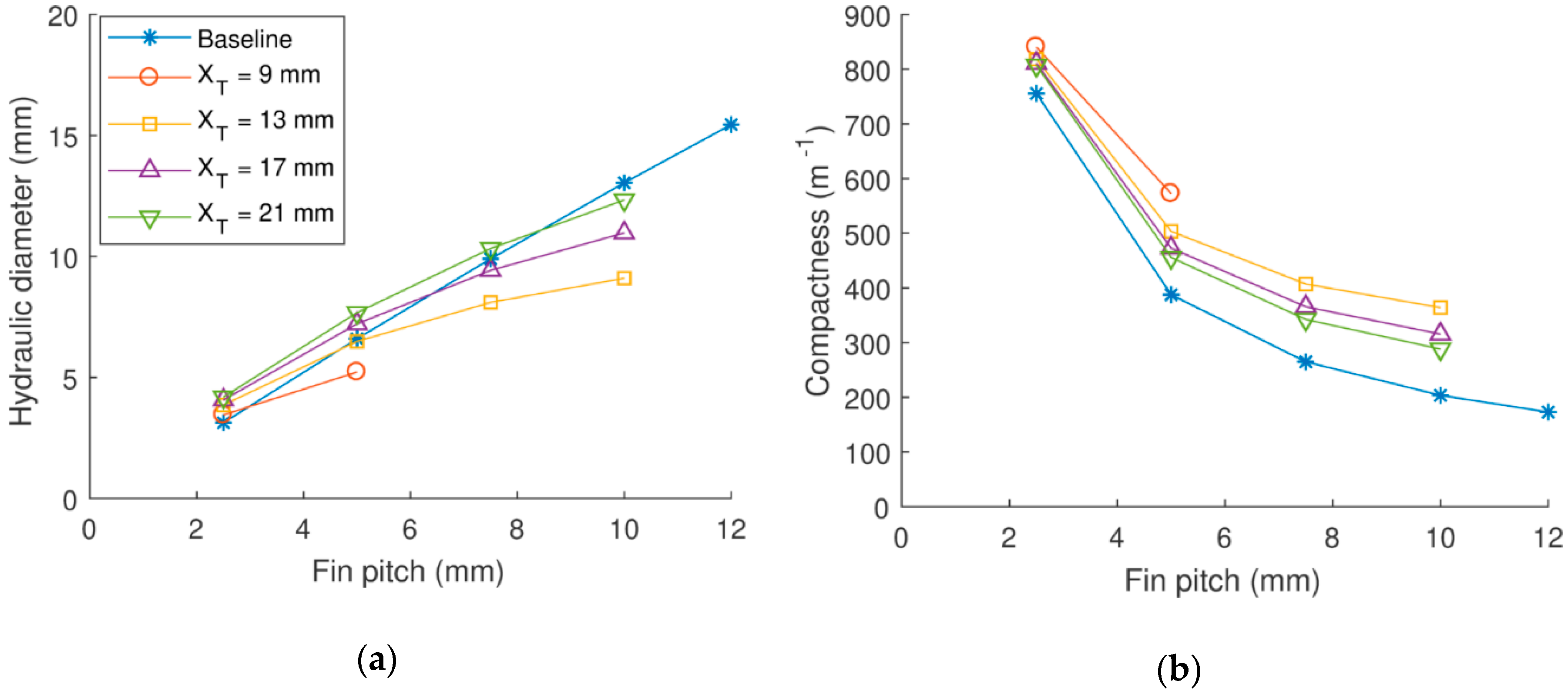
2.2. CFD Simulation Points
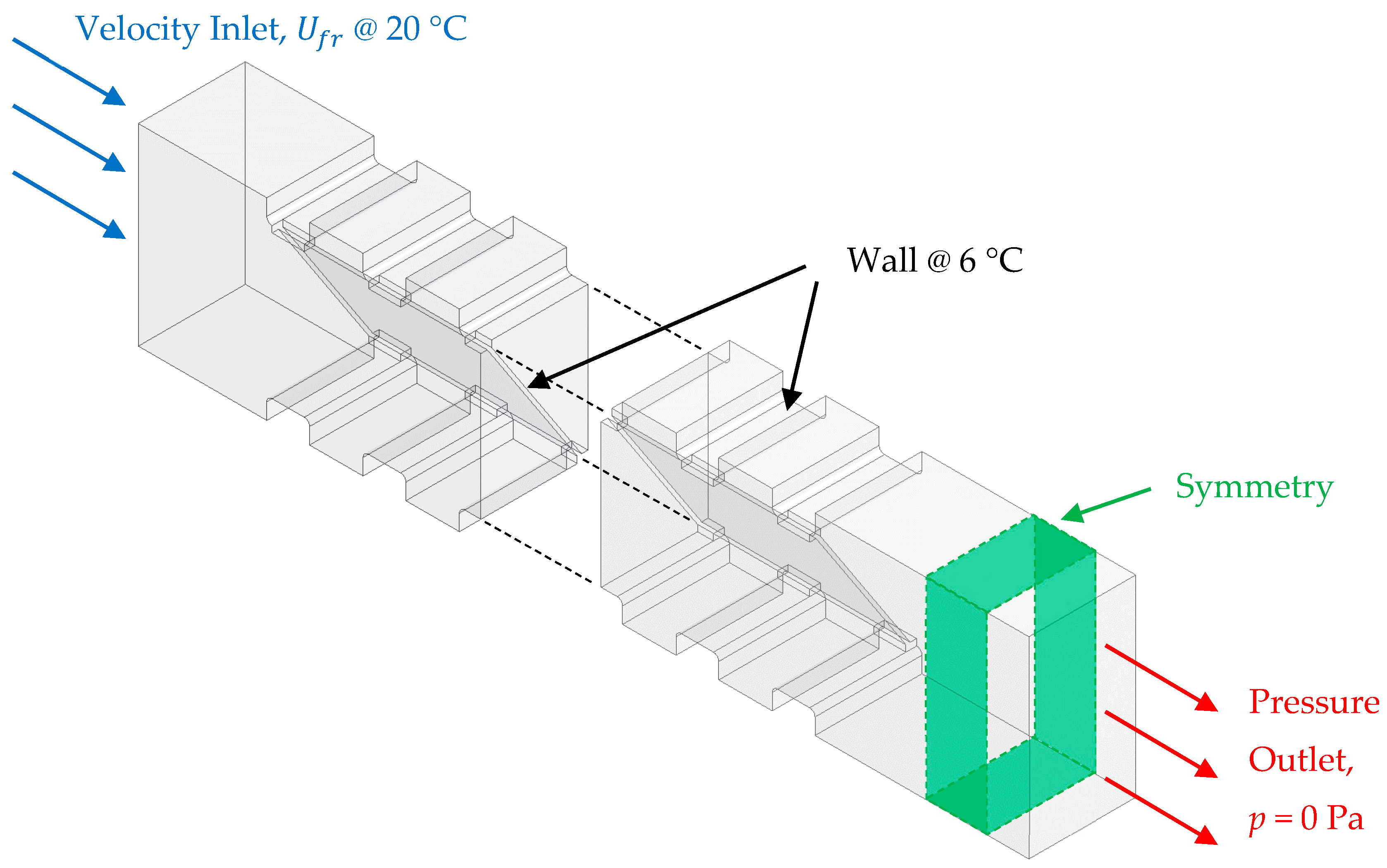
2.3. CFD Modeling Setup
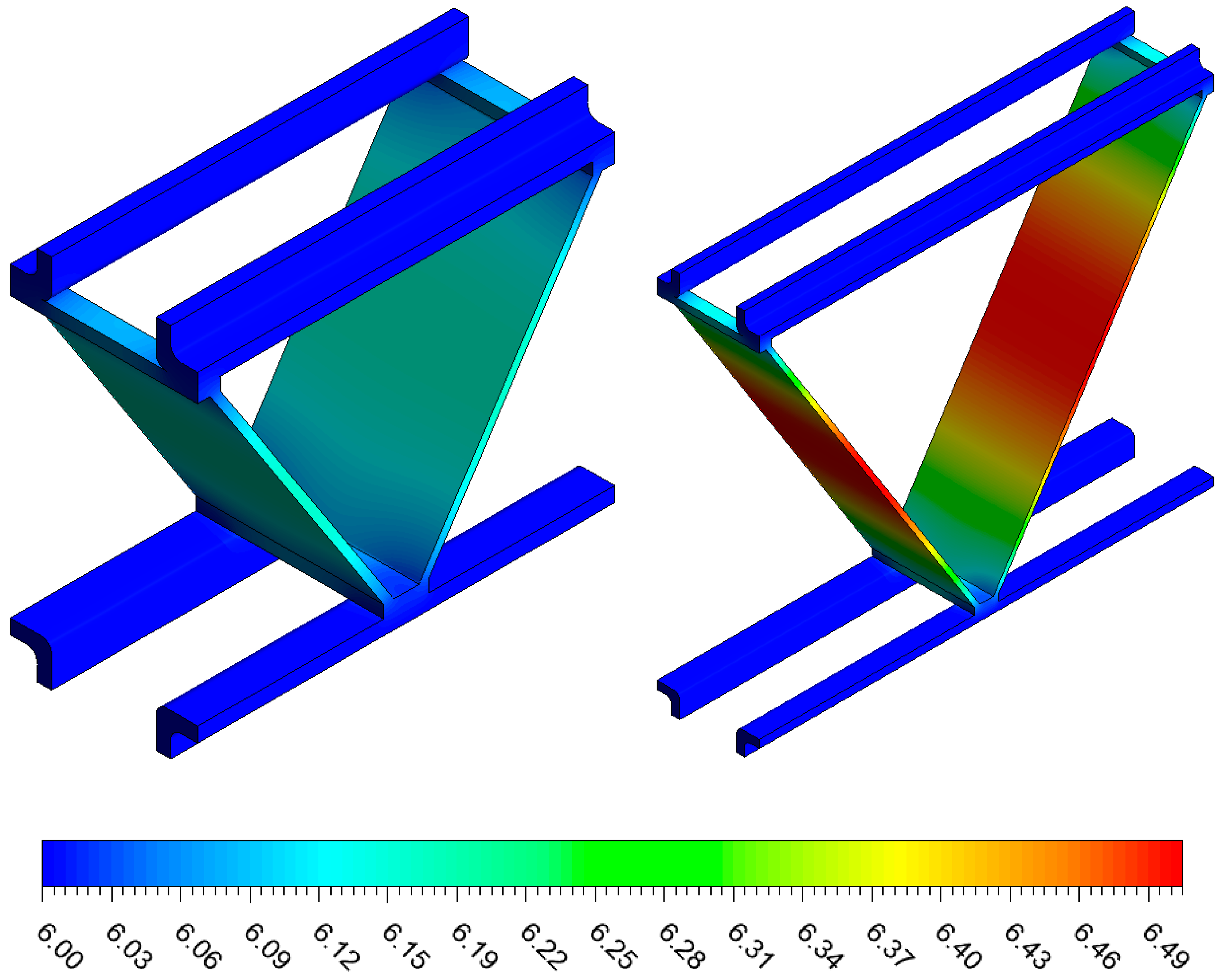
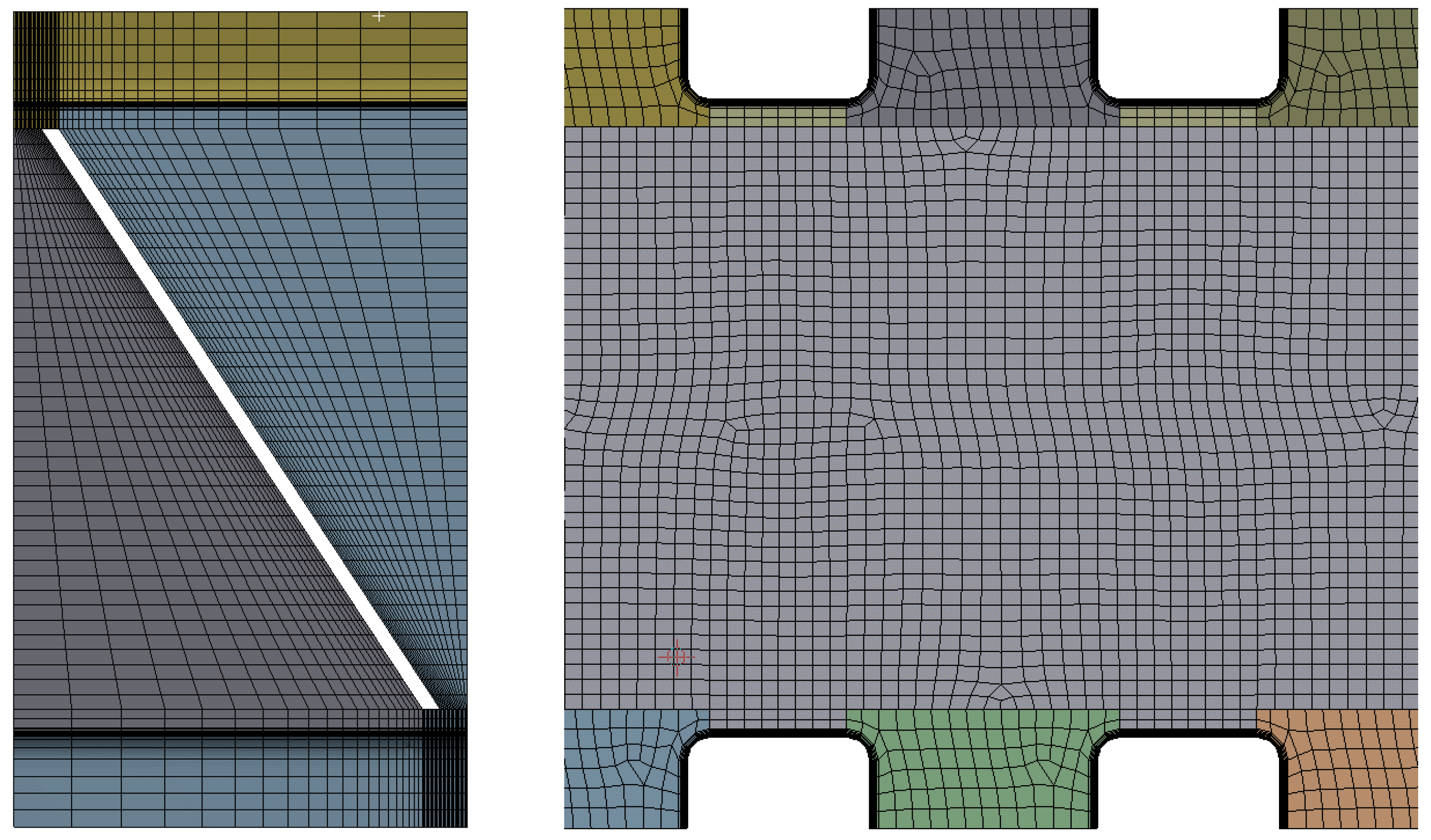
2.3.1. Modeling
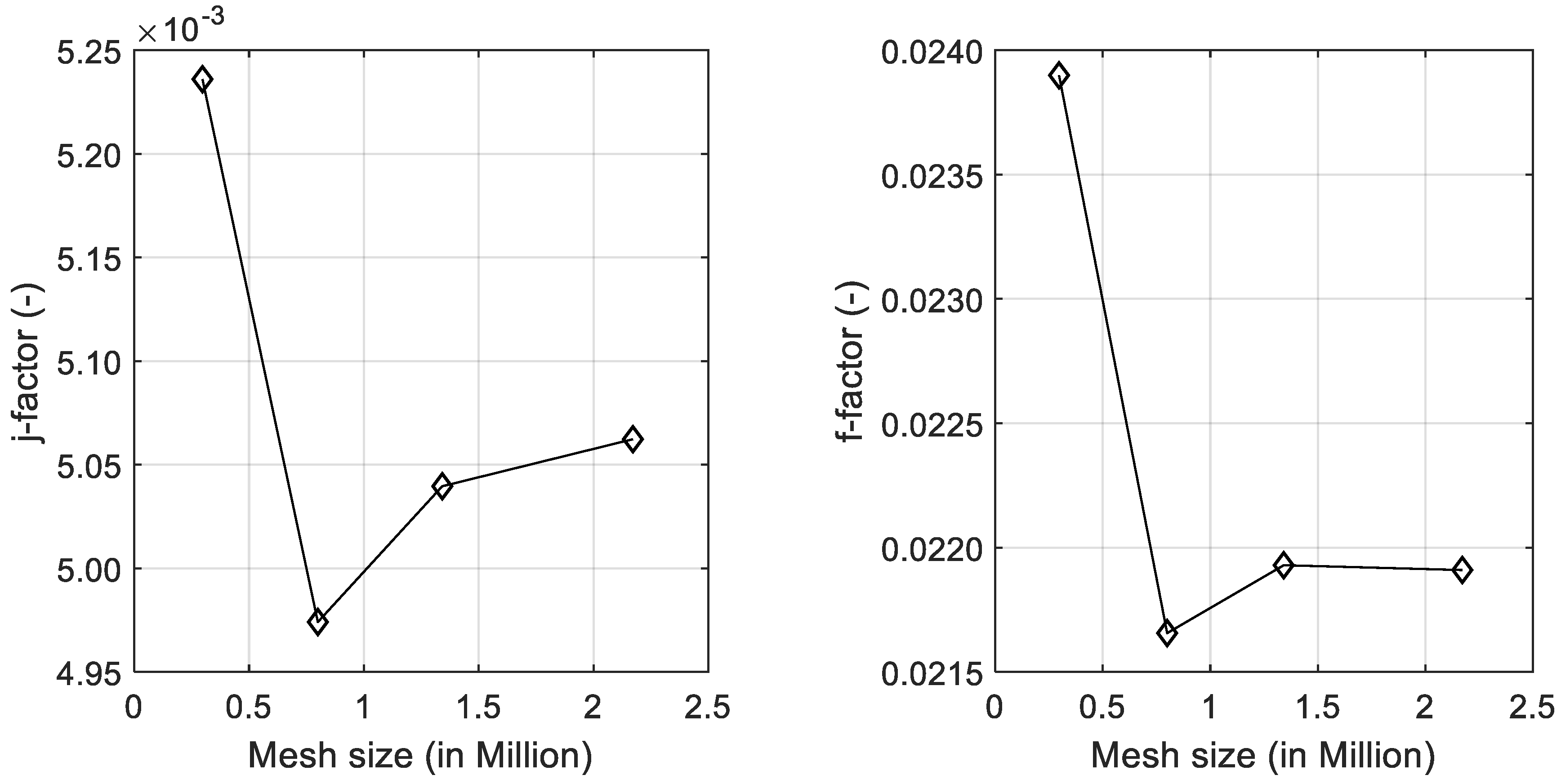
2.3.2. Mesh Analysis
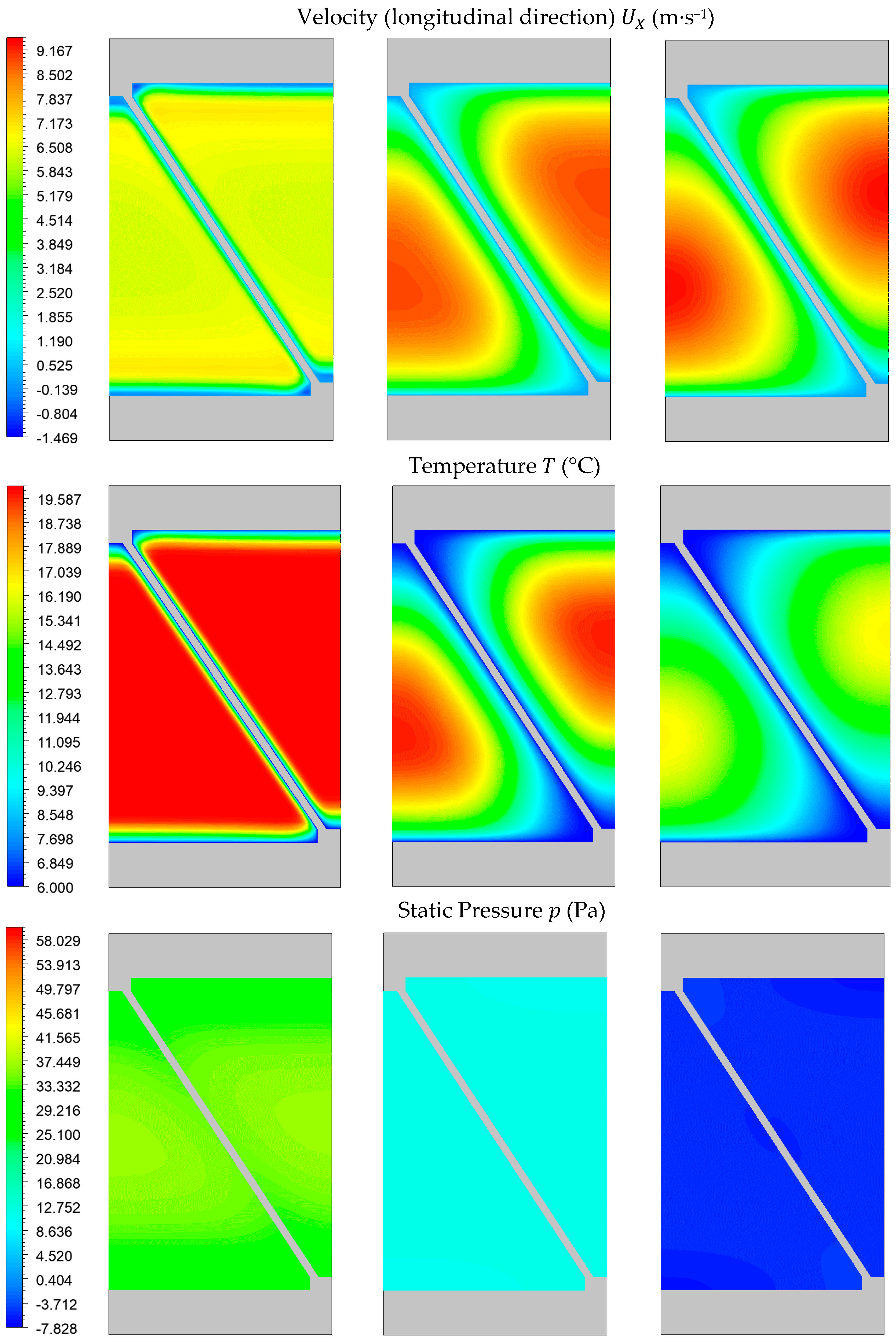
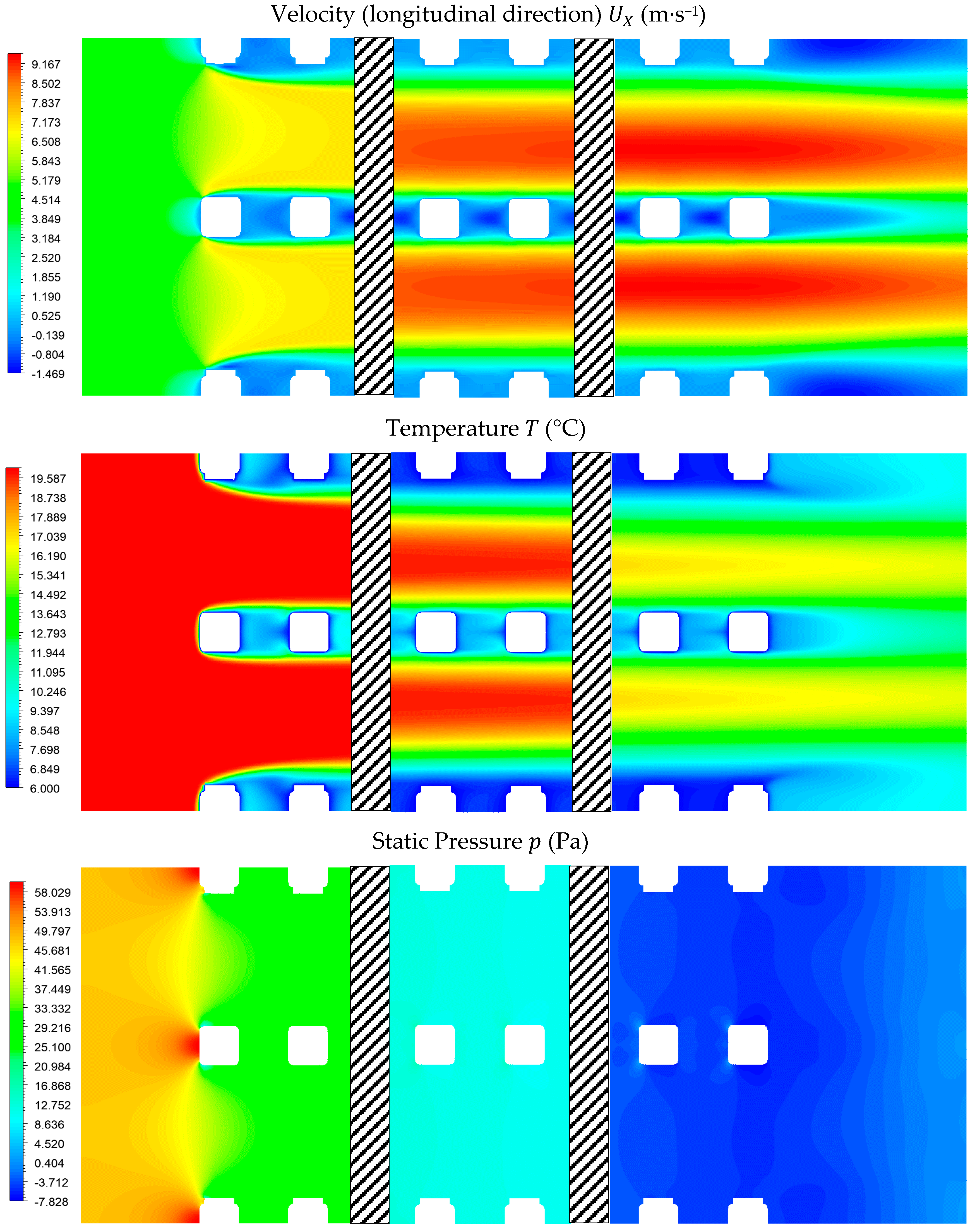
2.3.3. Velocity, Temperature, and Pressure Profiles
2.4. Data Reduction
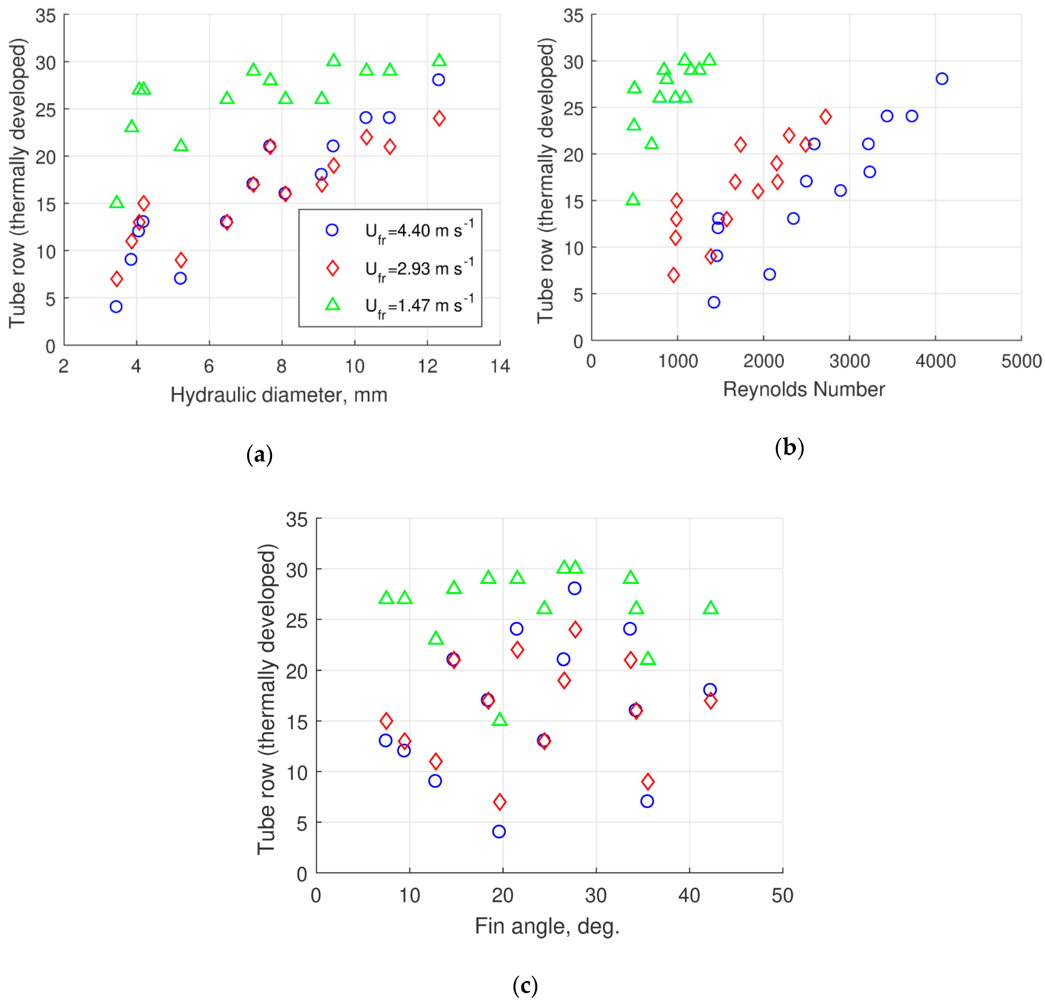
3. Results
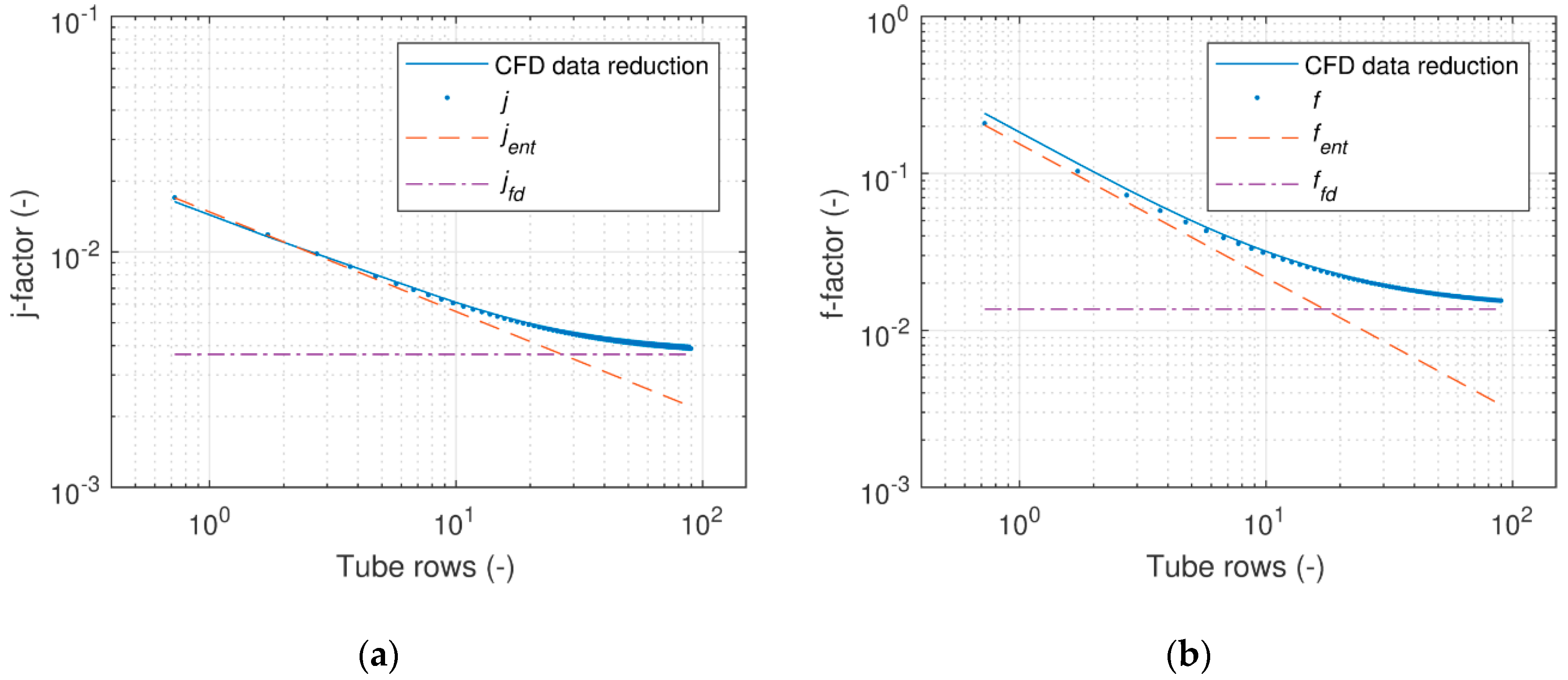
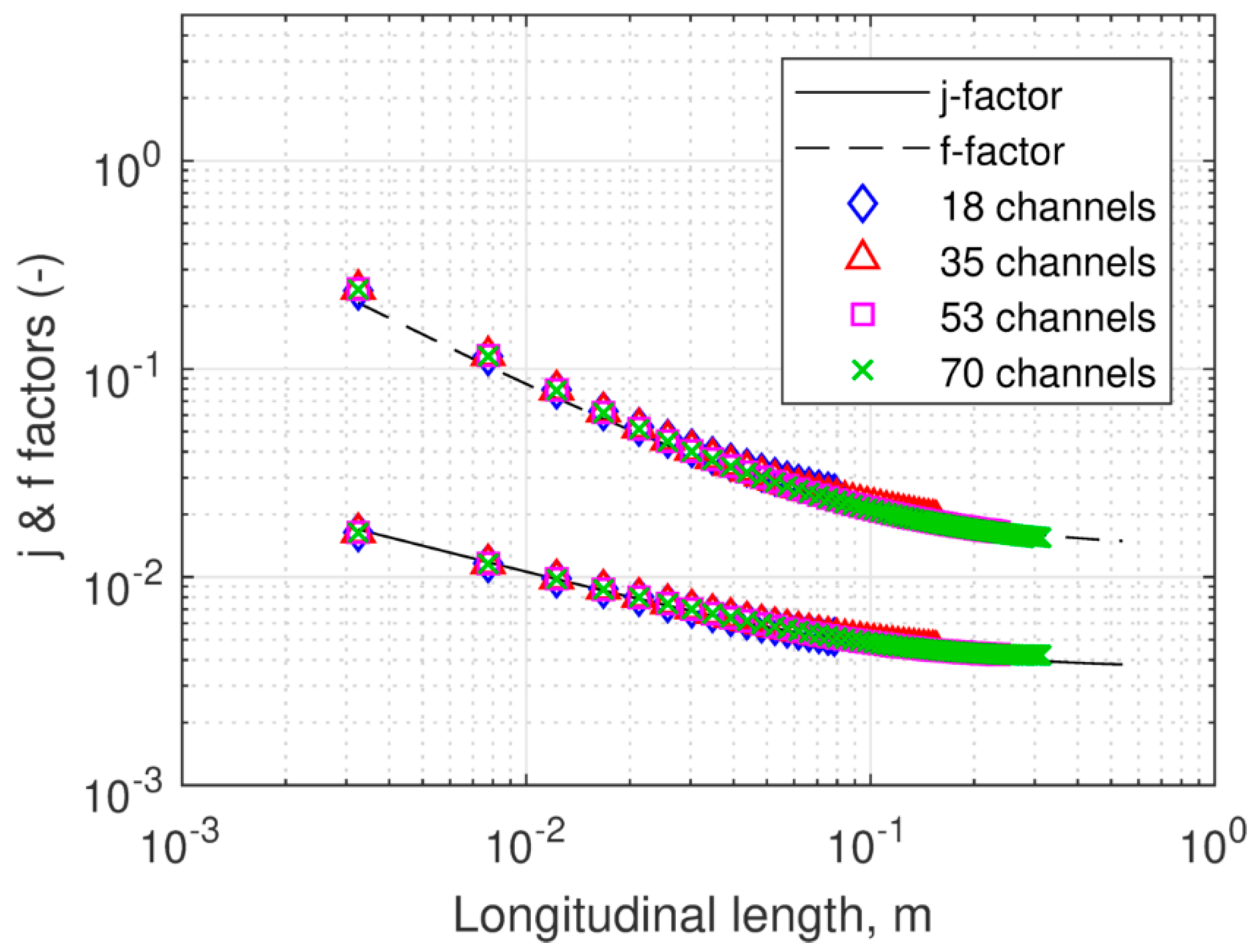
3.1. Heat Transfer and Pressure Drop Regression
- Linear regression of based on the first five consecutive points longitudinally (the choice of five points was based on visual interpretation of the results),
- Linear regression of ,
- Nonlinear regression of ,
- A repeated nonlinear regression of the coefficients and in order to alleviate errors related to the visual interpretation in step 1.
3.2. Analysis of Entrance Region
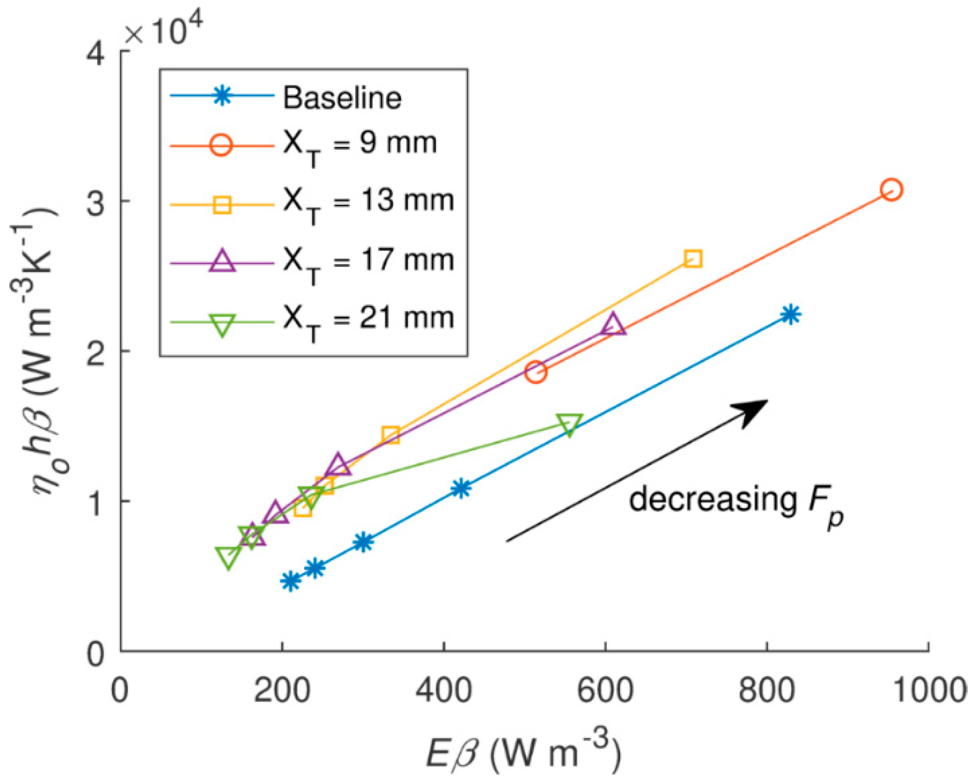
3.3. Volume Goodness Factor
4. Discussion
5. Conclusions
Author Contributions
Funding
Acknowledgments
Conflicts of Interest
Nomenclature
| Minimum free flow area, m2 | |
| Fin Area, m2 | |
| Frontal area, m2 | |
| Total heat transfer area, m2 | |
| Regression coefficients, (-) | |
| Heat capacity at constant pressure, J kg−1K−1 | |
| Lowest heat capacity rate, W K−1 | |
| Hydraulic diameter, m | |
| Friction power per unit surface area W m−2 | |
| f | Friction factor, (-) |
| Fin pitch, m | |
| Fin thickness, m | |
| Maximum mass velocity, kg s−1m−2 | |
| h | Heat transfer coefficient, W m−2K−1 |
| j | Colburn factor, (-) |
| Thermal conductivity of fin, W m−1K−1 | |
| Expansion and Contraction coefficient, (-) | |
| Tube rows, (-) | |
| Longitudinal length, m | |
| Transverse length, m | |
| Pressure, Pa | |
| Fin perimeter, m | |
| Prandtl number, (-) | |
| Heat transfer to the fin, W | |
| Heat transfer to an ideal fin, W | |
| R2 | Coefficient of determination, (-) |
| Re | Reynolds number, (-) |
| Tube height, m | |
| Tube width, m | |
| T | Temperature, K |
| Fluid ambient temperature, K | |
| Fin base temperature, K | |
| Fin average temperature, K | |
| Maximum air velocity, m s−1 | |
| Frontal air velocity, m s−1 | |
| Flow velocity in x-direction, m s−1 | |
| Longitudinal tube pitch, m | |
| Transverse tube pitch, m | |
| Dimensionless distance to the wall, (-) | |
| Greek Symbols | |
| Compactness, m−1 | |
| Fin efficiency, (-) | |
| Overall surface efficiency, (-) | |
| Viscosity, Pa s−1 | |
| Fluid density, kg m−3 | |
| Contraction ratio, (-) | |
| Fin angle, deg | |
| Pressure drop, Pa | |
| Abbreviation | |
| CFD | Computational Fluid Dynamics |
| FEM | Finite Element Method |
| LES | Large Eddy Simulation |
| LMTD | Logarithmic Mean Temperature Difference |
| MAD | Mean Absolute Deviation |
| MRD | Mean Relative Deviation |
| NTU | Number of Transfer Units |
| SST | Shear Stress Transport |
| Subscripts | |
| ent | Entrance |
| fd | Fully developed |
| i | Inlet |
| m | Mean |
| o | Outlet |
| v | Vapor |
| w | Wall |
Appendix A
Appendix A.1. Fin Efficiency

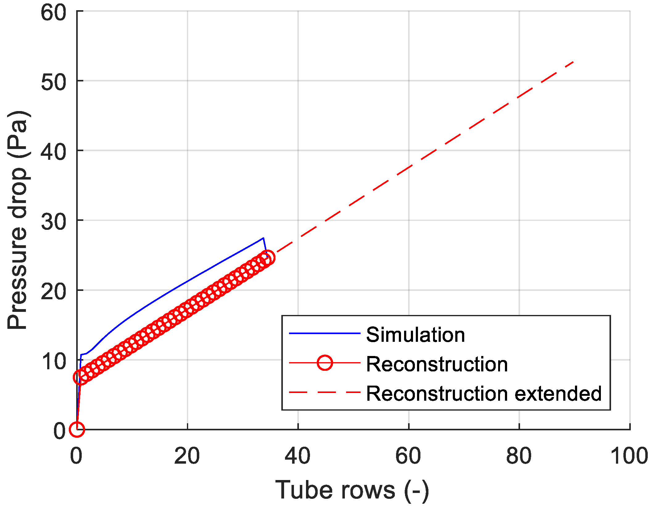
Appendix A.2. Longitudinal Extrapolation Analysis

References
- Ploug, O.; Vestergaard, B. New microchannel profile for evaporators and for refrigeration condensers. In Proceedings of the 4th International Congress on Aluminium Heat Exchanger Technologies for HVAC&R, Düsseldorf, Germany, 10–11 June 2015. [Google Scholar]
- Atkinson, K.N.; Drakulic, R.; Heikal, M.R.; Cowell, T.A. Two- and three-dimensional numerical models of flow and heat transfer over louvred fin arrays in compact heat exchangers. Int. J. Heat Mass Transf. 1998, 41, 4063–4080. [Google Scholar] [CrossRef]
- Perrotin, T.; Clodic, D. Thermal-hydraulic CFD study in louvered fin-and-flat-tube heat exchangers. Int. J. Refrig. 2004, 27, 422–432. [Google Scholar] [CrossRef]
- Qian, Z.; Wang, Q.; Cheng, J.; Deng, J. Simulation investigation on inlet velocity profile and configuration parameters of louver fin. Appl. Therm. Eng. 2018, 138, 173–182. [Google Scholar] [CrossRef]
- Sarpotdar, S.; Nasuta, D.; Aute, V.; Systems, O.; Road, V.M.; Park, C. CFD Based Comparison of Slit Fin and Louver Fin Performance for Small Diameter (3 mm to 5 mm) Heat Exchangers. Int. Compress. Eng. Refrig. Air Cond. 2016, 1988, 1–10. [Google Scholar]
- Jiang, Q.; Zhuang, M.; Zhu, Z.; Shen, J. Thermal hydraulic characteristics of cryogenic offset-strip fin heat exchangers. Appl. Therm. Eng. 2019, 150, 88–98. [Google Scholar] [CrossRef]
- Martinez, E.; Vicente, W.; Salinas-Vazquez, M.; Carvajal, I.; Alvarez, M. Numerical simulation of turbulent air flow on a single isolated finned tube module with periodic boundary conditions. Int. J. Therm. Sci. 2015, 92, 58–71. [Google Scholar] [CrossRef]
- Peng, H.; Ling, X.; Li, J. Performance investigation of an innovative offset strip fin arrays in compact heat exchangers. Energy Convers. Manag. 2014, 80, 287–297. [Google Scholar] [CrossRef]
- Bhuiyan, A.A.; Amin, M.R.; Naser, J.; Islam, A.K.M. Effects of geometric parameters for wavy finned-tube heat exchanger in turbulent flow: A CFD modeling. Front. Heat Mass Transf. 2015, 6, 1–11. [Google Scholar] [CrossRef] [Green Version]
- Ismail, L.S.; Velraj, R. Studies on fanning friction (f) and colburn (j) factors of offset and wavy fins compact plate fin heat exchanger-a CFD approach. Numer. Heat Transf. Part A Appl. 2009, 56, 987–1005. [Google Scholar] [CrossRef]
- Damavandi, M.D.; Forouzanmehr, M.; Safikhani, H. Modeling and Pareto based multi-objective optimization of wavy fin-and-elliptical tube heat exchangers using CFD and NSGA-II algorithm. Appl. Therm. Eng. 2017, 111, 325–339. [Google Scholar] [CrossRef]
- Cléirigh, C.T.Ó.; Smith, W.J. Can CFD accurately predict the heat-transfer and pressure-drop performance of finned-tube bundles? Appl. Therm. Eng. 2014, 73, 681–690. [Google Scholar] [CrossRef]
- Lindqvist, K.; Næss, E. A validated CFD model of plain and serrated fin-tube bundles. Appl. Therm. Eng. 2018, 143, 72–79. [Google Scholar] [CrossRef]
- Kemerli, U.; Kahveci, K. Numerical Investigation of Air-Side Heat Transfer and Fluid Flow in a Microchannel Heat Exchanger. In Proceedings of the 2nd World Congress on Mechanical, Chemical, and Material Engineering (MCM’16), Budapest, Hungary, 22–23 August 2016. [Google Scholar]
- Kumar, A.; Joshi, J.B.; Nayak, A.K.; Vijayan, P.K. 3D CFD simulations of air cooled condenser-III: Thermal-hydraulic characteristics and design optimization under forced convection conditions. Int. J. Heat Mass Transf. 2016, 93, 1227–1247. [Google Scholar] [CrossRef]
- Chennu, R.; Paturu, P. Development of heat transfer coefficient and friction factor correlations for offset fins using CFD. Int. J. Numer. Methods Heat Fluid Flow 2011, 21, 935–951. [Google Scholar] [CrossRef]
- Bacellar, D.; Aute, V.; Huang, Z.; Radermacher, R. Airside friction and heat transfer characteristics for staggered tube bundle in crossflow configuration with diameters from 0.5 mm to 2.0 mm. Int. J. Heat Mass Transf. 2016, 98, 448–454. [Google Scholar] [CrossRef] [Green Version]
- Deng, J. Improved correlations of the thermal-hydraulic performance of large size multi-louvered fin arrays for condensers of high power electronic component cooling by numerical simulation. Energy Convers. Manag. 2017, 153, 504–514. [Google Scholar] [CrossRef]
- Sadeghianjahromi, A.; Kheradmand, S.; Nemati, H. Developed correlations for heat transfer and flow friction characteristics of louvered finned tube heat exchangers. Int. J. Therm. Sci. 2018, 129, 135–144. [Google Scholar] [CrossRef]
- Patankar, S.V.; Liu, C.H.; Sparrow, E.M. Fully Developed Flow and Heat Transfer in Ducts Having Streamwise-Periodic Variations of Cross-Sectional Area. Trans. ASME. Ser. C, J. Heat Transf. 1977, 99, 180. [Google Scholar] [CrossRef]
- Martinez-Espinosa, E.; Vicente, W.; Salinas-Vazquez, M.; Carvajal-Mariscal, I. Numerical Analysis of Turbulent Flow in a Small Helically Segmented Finned Tube Bank. Heat Transf. Eng. 2017, 38, 47–62. [Google Scholar] [CrossRef]
- Awais, M.; Bhuiyan, A.A. Heat and mass transfer for compact heat exchanger (CHXs) design: A state-of-the-art review. Int. J. Heat Mass Transf. 2018, 127, 359–380. [Google Scholar] [CrossRef]
- Qasem, N.A.A.; Zubair, S.M. Compact and microchannel heat exchangers: A comprehensive review of air-side friction factor and heat transfer correlations. Energy Convers. Manag. 2018, 173, 555–601. [Google Scholar] [CrossRef]
- Kristófersson, J.; Vestergaard, N.P.; Skovrup, M.; Reinholdt, L. Ammonia charge reduction potential in recirculating systems—Calculations. In Proceedings of the IIR Ammonia Refrigeration Conference, Ohrid, Macedonia, 11–13 May 2017; pp. 80–87. [Google Scholar]
- Kristófersson, J.; Vestergaard, N.P.; Skovrup, M.; Reinholdt, L. Ammonia charge reduction potential in recirculating systems—System benefits. In Proceedings of the IIR Ammonia Refrigeration Conference, Ohrid, Macedonia, 11–13 May 2017; pp. 72–79. [Google Scholar]
- Lotfi, B.; Sundén, B. Development of new finned tube heat exchanger: Innovative tube-bank design and thermohydraulic performance. Heat Transf. Eng. 2019, 7632, 1–27. [Google Scholar] [CrossRef] [Green Version]
- Sahiti, N.; Lemouedda, A.; Stojkovic, D.; Durst, F.; Franz, E. Performance comparison of pin fin in-duct flow arrays with various pin cross-sections. Appl. Therm. Eng. 2006, 26, 1176–1192. [Google Scholar] [CrossRef]
- Menter, F.R. Two-equation eddy-viscosity turbulence models for engineering applications. AIAA J. 1994, 32, 1598–1605. [Google Scholar] [CrossRef] [Green Version]
- Kim, M.S.; Lee, J.; Yook, S.J.; Lee, K.S. Correlations and optimization of a heat exchanger with offset-strip fins. Int. J. Heat Mass Transf. 2011, 54, 2073–2079. [Google Scholar] [CrossRef]
- Chimres, N.; Wang, C.C.; Wongwises, S. Optimal design of the semi-dimple vortex generator in the fin and tube heat exchanger. Int. J. Heat Mass Transf. 2018, 120, 1173–1186. [Google Scholar] [CrossRef]
- Chapter 4: Turbulence, 4.16 Near-Wall Treatments for Wall-bounded Turbulent Flows, 4.16.1. In ANSYS Fluent 19.1 User’s Guide; ANSYS Inc.: Canonsburg, PA, USA, 2019.
- Shah, R.K.; Sekulic, D.P. Fundamentals of Heat Exchanger Design; John Wiley & Sons: Hoboken, NJ, USA, 2003. [Google Scholar]
- Webb, R.L.; Kim, N. Principles of Enhanced Heat Transfer, 2nd ed.; CRC Press: New York, NY, USA, 2005. [Google Scholar]
- Kaminski, U.; Grob, S. Luftseitiger Wärmeübergang und Druckverlust in Lamellenrohr-Wärmeübertragern. Ki Luft Kaeltetechnik 2000, 36, 13–18. [Google Scholar]
- Fraß, K.P.F.; Hofmann, R. Principles of Finned-Tube Heat Exchanger Design for Enhanced Heat Transfer, 2nd ed.; WSEAS Press, 2015; Available online: http://www.wseas.org/wseas/cms.action?id=9512 (accessed on 15 September 2019).
- Shah, R.K.; London, A.L. Laminar Flow Forced Convection in Ducts; Academic Press: New York, NY, USA, 1978. [Google Scholar]


| Parameters | Variation |
|---|---|
| Transverse tube pitch, (mm) | 9.00, 13.00, 17.00, 21.00 |
| Fin pitch, (mm) | 2.50, 5.00, 7.50, 10.00 |
| Longitudinal tube pitch, (mm) | 4.50 |
| Tube rows, (-) | 35 |
| Tube height, (mm) | 2.00 |
| Tube width, (mm) | 2.00 |
| Fin thickness, (mm) | 0.1625 |
| Frontal air velocity, (m·s−1) | 1.47, 2.93, 4.40 |
| Coefficient | j-Factor | f-Factor |
|---|---|---|
| 0.8539 | 0.8665 | |
| −0.5433 | −0.2804 | |
| −0.4234 | −0.8512 | |
| 0.0424 | 0.1777 | |
| −0.0966 | 0.9961 | |
| 0.0303 | 1.4393 | |
| −0.2697 | −0.5795 | |
| 0.1015 | −0.1196 | |
| 0.1095 | −0.2454 | |
| 3.1784 | 1.2611 |
© 2019 by the authors. Licensee MDPI, Basel, Switzerland. This article is an open access article distributed under the terms and conditions of the Creative Commons Attribution (CC BY) license (http://creativecommons.org/licenses/by/4.0/).
Share and Cite
Rogie, B.; Brix Markussen, W.; Honore Walther, J.; Ryhl Kærn, M. Numerical Investigation of Air-Side Heat Transfer and Pressure Drop Characteristics of a New Triangular Finned Microchannel Evaporator with Water Drainage Slits. Fluids 2019, 4, 205. https://doi.org/10.3390/fluids4040205
Rogie B, Brix Markussen W, Honore Walther J, Ryhl Kærn M. Numerical Investigation of Air-Side Heat Transfer and Pressure Drop Characteristics of a New Triangular Finned Microchannel Evaporator with Water Drainage Slits. Fluids. 2019; 4(4):205. https://doi.org/10.3390/fluids4040205
Chicago/Turabian StyleRogie, Brice, Wiebke Brix Markussen, Jens Honore Walther, and Martin Ryhl Kærn. 2019. "Numerical Investigation of Air-Side Heat Transfer and Pressure Drop Characteristics of a New Triangular Finned Microchannel Evaporator with Water Drainage Slits" Fluids 4, no. 4: 205. https://doi.org/10.3390/fluids4040205