Cloud-Based CAD Parametrization for Design Space Exploration and Design Optimization in Numerical Simulations

Abstract

In this manuscript, an automated framework dedicated to design space exploration and design optimization studies is presented. The framework integrates a set of numerical simulation, computer-aided design, numerical optimization, and data analytics tools using scripting capabilities. The tools used are open-source and freeware, and can be deployed on any platform. The main feature of the proposed methodology is the use of a cloud-based parametrical computer-aided design application, which allows the user to change any parametric variable defined in the solid model. We demonstrate the capabilities and flexibility of the framework using computational fluid dynamics applications; however, the same workflow can be used with any numerical simulation tool (e.g., a structural solver or a spread-sheet) that is able to interact via a command-line interface or using scripting languages. We conduct design space exploration and design optimization studies using quantitative and qualitative metrics, and, to reduce the high computing times and computational resources intrinsic to these kinds of studies, concurrent simulations and surrogate-based optimization are used.

1. Introduction

Consumer demand, government regulations, competitiveness, globalization, better educated end-users, environmental concerns, market differentiation, social media trends, and even influencers, they are all driving products manufacturers and industry to reduce production expenditures and final cost of goods, and at the same time improving the quality and reliability of the products with the lowest environmental impact. To reach these goals and to develop revolutionary products, the manufacturing sector is relying more on virtual prototypes, computer simulations, and design optimization.

Computational fluid dynamics (CFD), computational structural dynamics (CSD), computer-aided manufacturing (CAM), computer-aided design (CAD), multi-physics simulations, digital twins, the internet-of-things (IoT) and the cloud, are among many of the tools increasingly being used to simulate and certify products by analysis and simulation before going into production and commercialization. Even before reaching the market, modern products have undergone some kind of heuristic or methodological optimization. Though the optimization might take different forms in different fields (e.g., finance, health, construction, operations, manufacturing, transportation, construction, engineering design, sales, public services, mail, and so on), the ultimate goal is always getting the best out of something under given circumstances, either by minimizing, maximizing, equalizing, or zeroing a quantity of interest (QoI).

Product optimization can be undertaken in two different ways, by using design space exploration (DSE) or by using design optimization (DO). Even a combination of both methodologies is possible. In DSE, we simply explore the design space in a methodological way, and while doing so, we extract knowledge. DSE is the process of discovering, expanding, evolving, and navigating the design space to extract knowledge to support better decision making [1]. It is not difficult to recognize that in DSE, we are not converging to an optimal value, we are only exploring the design space, but in doing so, we are gathering valuable information about the global behavior, and this information can be used to get a better design. Moreover, this knowledge can also be used to conduct surrogate-based optimization (SBO) studies. The SBO method consists of constructing a mathematical model (also known as a surrogate, response surface, meta-model, emulator) from a limited number of observations (CFD simulations, physical experiments, or any quantifiable metric) [2,3,4,5]. After building the surrogate, it can be explored and exploited. Conducting the optimization at the surrogate level is orders of magnitude faster than working at the high fidelity level [2].

Design optimization strategies, on the other hand, consist on formulating an optimization problem and converging to the optimal design. Here, it is assumed that the problem can be formulated before the search and convergence begin. A typical optimization problem can be formulated as follows,

$$\begin{array}{c}\hfill \mathrm{Find}\mathbf{X}=\left\{\begin{array}{c}{x}_1\\ x_2\\ ⋮\\ x_n\end{array}\right\}\end{array}$$

(1)

which minimizes, maximizes, equalizes, or zeroed,

$$\begin{array}{c}\hfill f_j\left(\mathbf{X}\right),j=1,2,\cdots ,q\end{array}$$

(2)

subject to design constraints (linear and non-linear),

$$\begin{array}{cc}\hfill & g_j\left(\mathbf{X}\right)\le 0,j=1,2,\cdots ,m\hfill \\ \hfill & l_j\left(\mathbf{X}\right)=0,j=1,2,\cdots ,p\hfill \end{array}$$

(3)

and variables bounds,

$$\begin{array}{cc}\hfill & x_i^{lb}\le x_i\le x_i^{ub}j=1,2,\cdots ,n\hfill \end{array}$$

(4)

where $\mathbf{X}$ is a n-dimensional vector called the design vector, $f_j\left(\mathbf{X}\right)$ is the objective function or QoI, $g_j\left(\mathbf{X}\right)$ are the inequality constraints, $l_j\left(\mathbf{X}\right)$ are the equality constraints, and $x_i^{lb}$ and $x_i^{ub}$ are the variables lower and upper bounds, respectively. To find the optimal value we can use gradient-based methods or derivative-free methods [5,6,7,8,9,10]. Also, the problem formulation can be single-objective (one QoI to be optimized) or multi-objective (more than one QoI to be optimized simultaneously). Things can get even more complicated, as in some cases we might need to deal with design optimization problems incorporating many disciplines (e.g., aerodynamics, propulsion, structures, and performance). In this case, we say we are dealing with a multi-disciplinary design optimization problem (MDO) [11,12,13,14,15,16]. MDO allows designers and engineers to incorporate all relevant disciplines simultaneously. The optimum of the simultaneous problem is superior to the design found by optimizing each discipline sequentially since it can exploit the interactions between the disciplines. However, including all disciplines simultaneously significantly increases the complexity of the problem [7].

The field we are concerned with in this manuscript is that of engineering design; nevertheless, this by no means limits the range of applicability of the current work; it simply reflects the authors’ interests and fields of expertise.

In engineering design, we are often interested in optimizing the geometry. To do so, two approaches are available, direct modeling and parametric modeling. In direct modeling, we modify the geometry by pushing and pulling points, lines, and surfaces (like working with clay). This gives designers and engineers a lot of flexibility when it comes to shape the geometry; however, in the process of doing so, we give up geometry parametrization in favor of creating organic shapes that might be difficult to manufacture. In parametric modeling, the user defines relationships, constraints, parametric variables, and configurations when creating the solid model. Then, by changing these variables, the user can easily create endless variations on the original geometry with complete control and millimetric precision.

However, when conducting fully automatic DSE or DO studies, introducing the CAD tools is not very straightforward. Most of the times the CAD applications are not compatible with the operating system (OS) where the numerical simulations are being performed (usually Unix-like OS), or simply, it is not possible to connect the optimization loop with the CAD tool due to the fact that the user can only interact with it using a graphical user interface (GUI), which cannot be used in an automatic optimization loop driven by a command-line interface (CLI).

To overcome this problem, many commercial simulation frameworks are adding a monolithic design environment to integrate all the applications needed to conduct design space exploration and design optimization studies, namely CAD, multi-physics solver, optimizer, and post-processing. While commercial frameworks have proven to be reliable, they come with a price tag that often is unreachable by small and medium-sized enterprises (SMEs), hobbyists, researchers or personal users. Hereafter, we propose the integration of open-source and freeware tools to conduct DSE and DO studies.

To perform the numerical simulations, we use the multi-physics solver OpenFOAM (version 7.0) [17,18] or the programming language Python. The optimization algorithms and the code coupling interface is provided via the Dakota library [19,20] (version 6.10). All the real-time data analytics, quantitative and qualitative post-processing, and data analytics are performed using Python, VTK [21], and bash scripting. Finally, to create and modify the geometry we use Onshape [22], which is a cloud-based parametric CAD and product development application. Onshape’s application programming interface (API) is open-source; therefore, it can be deployed in any platform with an internet connection. The API is implemented in Python, and the calls to Onshape’s server are done using RESTful requests. Onshape offers two subscription plans, a pay-up plan and a free one. Both subscriptions plans have the same professional capabilities, the only difference is the level of product support offered and the access to enterprise options.

The purpose of this manuscript is two-fold. First, we want to use the cloud to support CAD parametrization in DSE or DO design loops, which undoubtedly will give users enormous flexibility as the CAD application does not need to be installed locally, and there is no need for a monolithic CAD/Simulation software integration. Secondly, we want to deploy fully automatic, fault-tolerant, and scalable engineering design loops using in-house computational resources, the cloud, or HPC centers; and everything based on open-source and freeware tools. We hope that this contribution will offer guidelines to designers and engineers working with design optimization and design space exploration, will help them at implementing their own optimization loops, and to some extent, it will help to address some of the findings and recommendations listed in the NASA contractor report “CFD Vision 2030 Study: A Path to Revolutionary Computational Aerosciences” [23], where it is stated the following: “Included in this desired set of capabilities is a vision for how CFD in 2030 will be used: a vision of the interaction between the engineer/scientist, the CFD software itself, its framework and all the ancillary software dependencies (databases, modules, visualization, etc.), and the associated HPC environment. A single engineer/scientist must be able to conceive, create, analyze, and interpret a large ensemble of related simulations in a time-critical period (e.g., 24 h), without individually managing each simulation, to a pre-specified level of accuracy”.

The rest of the manuscript is organized as follows. Section 2 gives an overview of the methodology used. In Section 3 we describe the numerical experiments carried out to demonstrate the usability and flexibility of the framework. Finally, in Section 4 we present the conclusions and future perspectives.

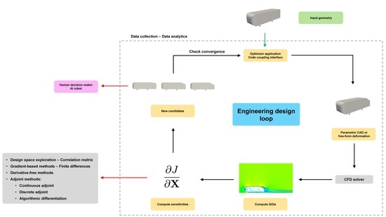
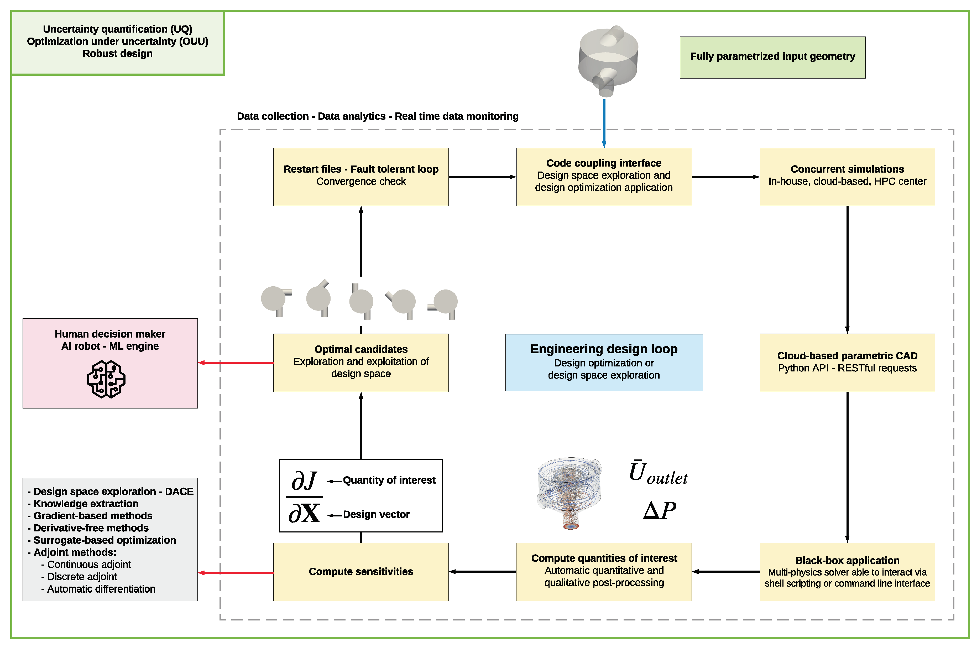
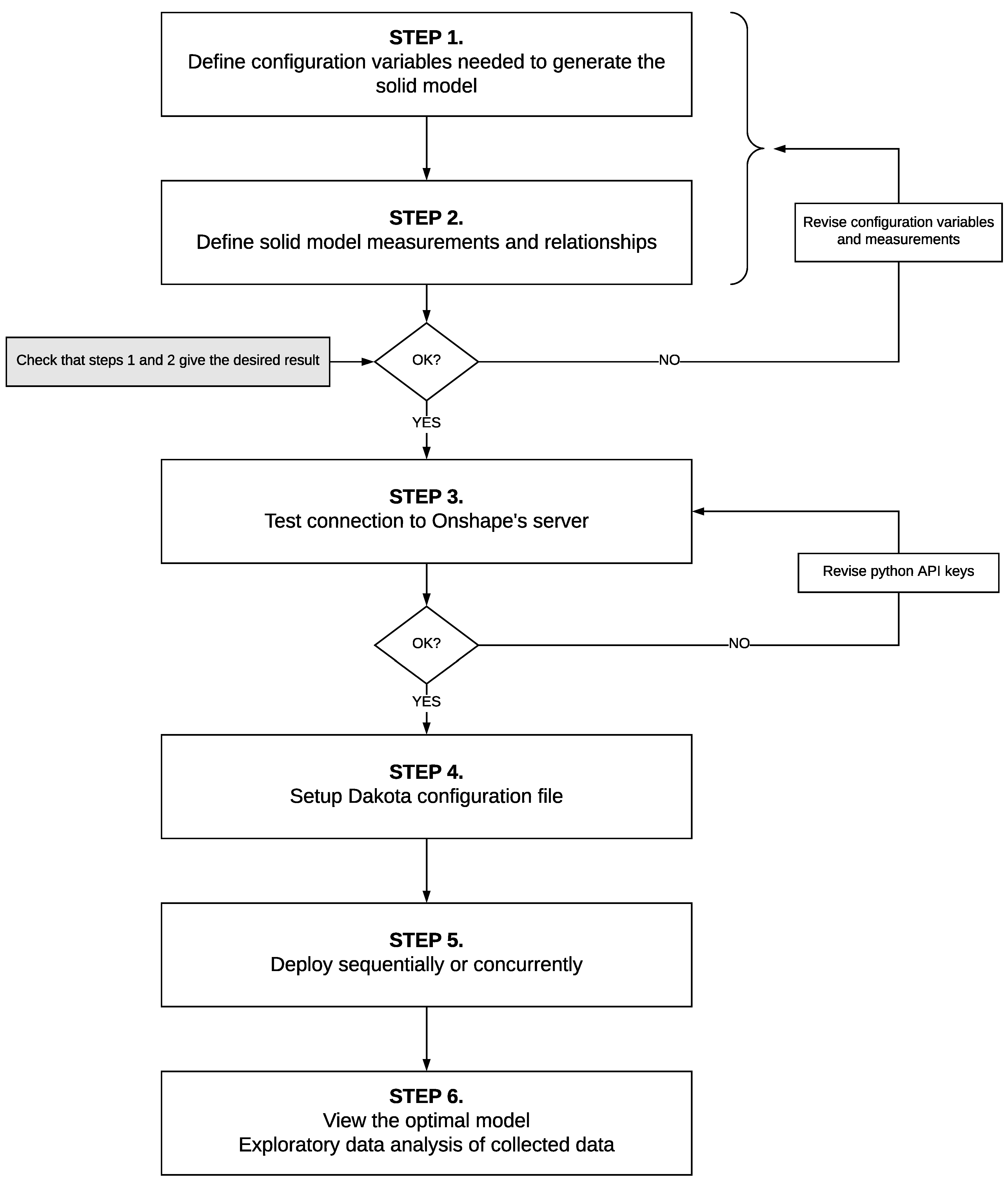
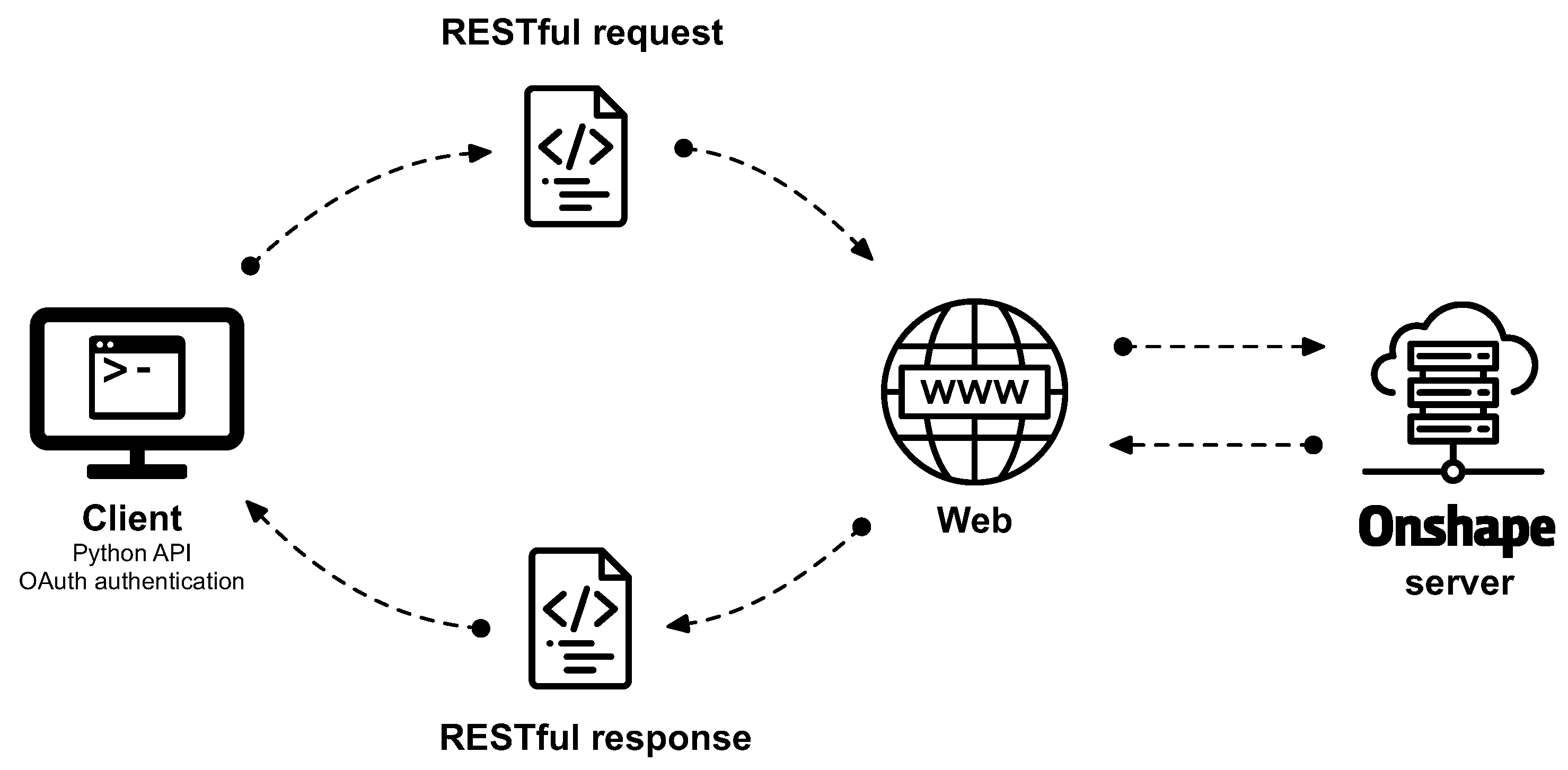
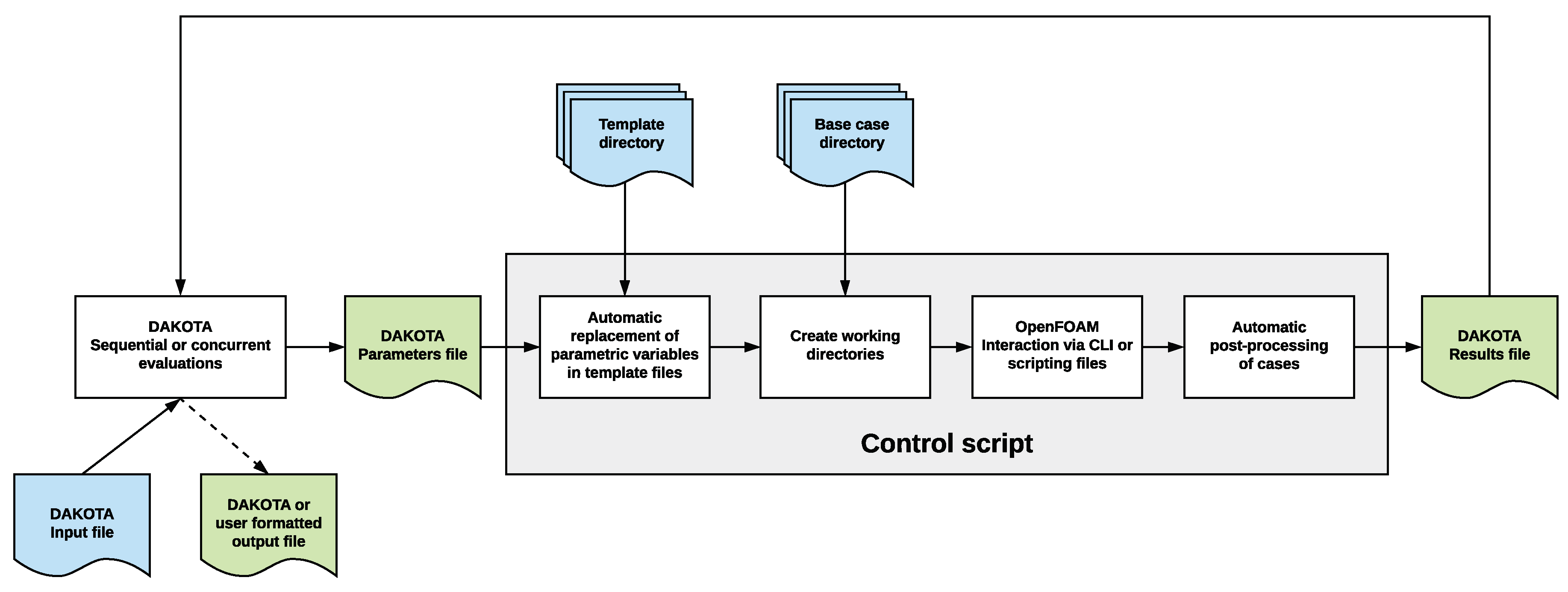
2. Description of the Workflow—Methodology

In Figure 1, we illustrate a graphical summary of the methodology used in this work. The engineering design loop starts with a fully parametrized geometry, then new candidates are generated by changing the parametrical variables. It is important to stress that our starting point is the parametrical variables and not the solid model; that is, we are allowed to start from any possible geometry that can be generated using the parametrical variables. Hereafter, we use Onshape [22] as solid modeler, which is a cloud-based CAD application. The fact that Onshape is cloud-based gives us the flexibility to deploy the framework in any platform without the need to install the application. The only requirement is to have a working internet connection.

The whole workflow is controlled by the library Dakota [19,20], which serves as the numerical optimizer and code coupling interface tool. The Dakota library provides a flexible and extensible interface between simulation codes and iterative analysis methods. The library is software agnostic, in the sense that it can interface any application that is able to parse input/output files via a CLI. The library also has extensive design optimization and design space exploration capabilities. It comes with many gradient-based methods and derivative-free methods for design optimization. It also contains many design and analysis of computer experiments (DACE) methods to conduct design space exploration studies. And to obtain faster turn-around times, Dakota supports concurrent function evaluations.

The engineering design loop illustrated in Figure 1 is orchestrated by using Dakota’s configuration input file. In this input file, all the steps to follow in the engineering design loop are defined. As previously stated, the only requirement is that the applications involved in the loop can interact via the CLI. In references [3,24,25,26,27,28,29,30,31,32,33], few examples using Dakota to control complex engineering design loops are discussed. However, none of them addressed the use of a fully parametric cloud-based CAD tool to generate the solid geometry or the use of the cloud to deploy the loop.

After defining Dakota’s configuration file, the engineering design loop can be launched sequentially or concurrently using local resources, on the cloud, or remotely in an HPC center. All the tools involved in the loop are black-box applications that are connected using Dakota. An essential step of every optimization loop is that a QoI must be provided to compute the sensitivities; this is also controlled using Dakota’s configuration file. This step is critical and is the user’s responsibility to define all the quantities of interests to monitor. After computing the QoI, Dakota will compute the sensitivities using the method selected by the user. With Dakota, the user is not obliged to use the optimization and space exploration methods implemented on it; one can easily interface Dakota with a third-party optimization library.

At this point, we can rely on a human decision-maker or a machine learning engine to pick up the best design or set of optimal solutions. During the whole process, data is collected and monitored in real time. Dakota also offers restart capabilities, so in the event of an unexpected failure of the system (hardware or software), the user can restart from a previously saved state.

In this work, we use the design loop illustrated in Figure 1 for DO and DSE studies. In DO, the user starts from an initial design or guess, and the optimization algorithm will make it slightly better, i.e., in DO we are making sub-optimal guesses incrementally better. This by no means is negative, and the chances are that the results are a substantial improvement over the initial guess. In essence, DO is an iterative-converging process that requires a starting point (or a set of points) and a set of constraints. On the other hand, in DSE we do not need to define an initial guess or a set of constraints (except for the bounds of the design space). We generate new solutions sequentially or concurrently that might be better or worse than a baseline, but in the process of doing so, we are exploring and exploiting the design space. DSE gives more information to engineers than DO, and this information can be used for decision making, knowledge extraction, and anomalies detection. All the information gathered during the design loop can also be used to construct reduced-order models, surrogate models, or to interrogate the data using exploratory data analysis and machine learning techniques.

3. Numerical Experiments

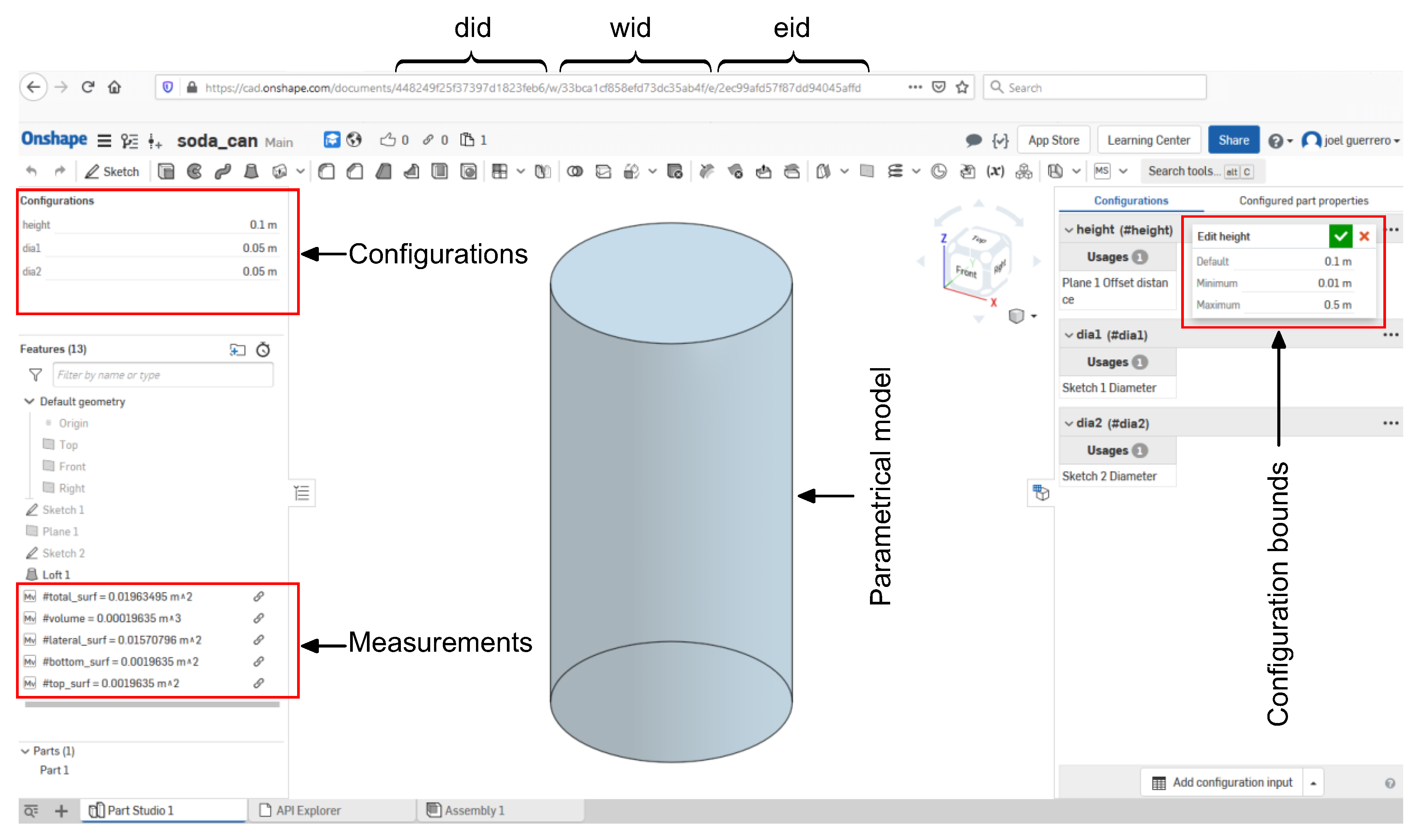
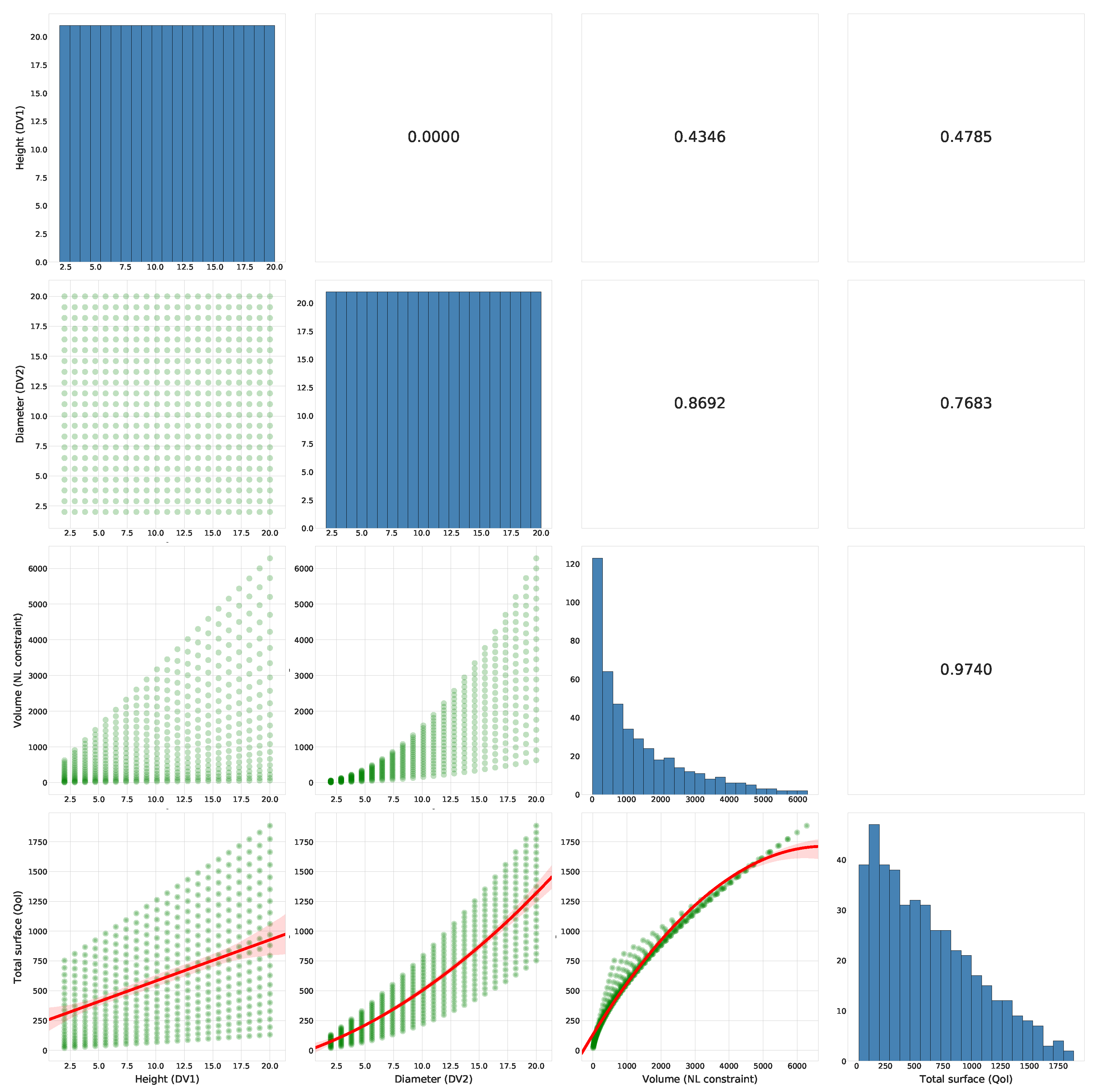
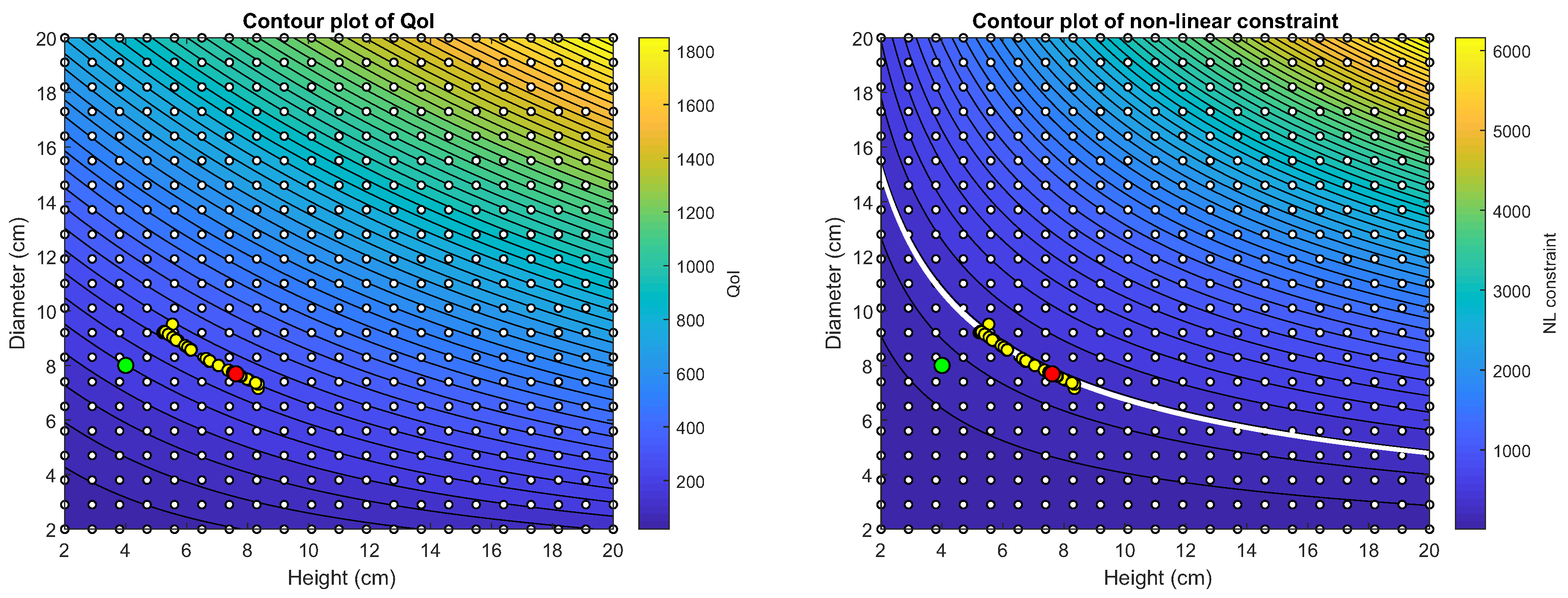
3.1. Cylinder Optimization Problem—Minimum Surface and Fixed Volume

This problem is also known as the soda can optimization problem. We aim at finding the optimal dimensions of a right cylinder that minimize the total surface area of the cylinder, which holds a given volume. This problem can be formulated as follows,

$$\begin{array}{c}\hfill \mathrm{minimize}{S}_{tot}\end{array}$$

(5)

subject to,

$$\begin{array}{c}\hfill V=355{\mathrm{cm}}^3\\ \hfill 0<r,h<\infty \end{array}$$

(6)

where

$$\begin{array}{cc}\hfill S_{tot}& =2\pi r^2+2\pi rh\hfill \\ \hfill V& =\pi r^{2}h\hfill \end{array}$$

(7)

in Equations (5)–(7), $S_{tot}$ is the cylinder’s total surface, V its volume, r its radius, and h its height. The solution to this problem is the following,

$$\begin{array}{cc}\hfill r& =3.837\mathrm{cm}\hfill \\ \hfill h& =7.675\mathrm{cm}\hfill \\ \hfill S_{min}& =277.54{\mathrm{cm}}^2\hfill \end{array}$$

(8)

This is a classic problem that is frequently posed to first-year calculus students. Therefore, we will not go into details on how to find the analytical solution (Equation (8)). Instead, we will use this case to illustrate how the cloud-based design loop works.

In Figure 2, we illustrate the general workflow. In steps 1–2, we define all the configuration variables and measurements (e.g., area, volume, length, and so on). In these steps, we also check that we are obtaining the desired output by changing manually the parametrical variables. In Figure 3, we show the screen-shot of how this case was setup in Onshape (the document is available at the following link https://cad.onshape.com/documents/448249f25f37397d1823feb6/w/33bca1cf858efd73dc35ab4f/e/2ec99afd57f87dd94045affd); in the figure, it can be observed that all the configurations, bounds, and measurements have been defined. All these variables can be accessed or modified using Onshape’s Python API (https://github.com/onshape-public/apikey/tree/master/python). In step 3 we proceed to test the connection with Onshape’s server, this is illustrated in Figure 4. In the figure, we use the API client to encode the changes to the model configurations and evaluation of the measurements. Then, using OAuth authentication, a RESTful request is sent to Onshape’s server, which sends a response back to the client. The response can be the new geometry or the evaluation of the volume of the new solid model. After testing the configurations and communication with Onshape’s server, we proceed to define the problem in Dakota’s configuration file and to create any additional scripts needed to parse input/output files (step 4). This step includes choosing the optimization or space exploration method and defining the bounds, constraints, and objective functions. At this point, we can proceed to deploy the case sequentially or concurrently using local resources, the cloud, or HPC center resources (step 5). Finally, in step 6, we can visualize the optimal solid model. Additionally, we can use exploratory data analysis to study the collected data. During the whole process, restart files are generated, and data is monitored in real time.

In Listing 1, we show an excerpt of the Python code used to change the configuration variables. In the listing, the keywords height_to_update, dia1_to_update, and dia2_to_update are the parametric variables, and each one was defined in the Onshape document. Their values are substituted automatically by Dakota, and their bounds are defined in Dakota’s configuration file. The function part_studio_stl_conf is responsible for exporting the geometry using the current values of the configuration variables (in this case the geometry is exported in STL format but any supported CAD exchange format can be used). The exported geometry is then used with the black-box solver. The did, wid, and eid keywords in Listing 1 are referred to the document id, workspace id, and element id of the Onshape document (refer to Figure 3). In Listing 2, we show an excerpt of the Python code used to evaluate the measurements (the structure is similar to that of Listing 1). In the listing, the line of code “function(context, queries) return getVariable(context, ’volume’);” evaluates the measurement, as defined in the Onshape document. In this case, we are evaluating the volume of the solid model. As for the configuration variables, all the measurements need to be defined in the Onshape document. In the listing, the function featurescript_conf takes the configuration values and the measurement function definition and gives as output the evaluation of the measurement for the given configuration. For the interested reader, the working case with all the scripts can be downloaded at this link (https://github.com/joelguerrero/cloud-based-cad-paper/tree/master/soda_can/). These scripts can be used as a starting point for more complex cases. It is worth mentioning that the Python API works with Python 2 (2.7.9+).

Let us discuss the outcome of a DO study using a gradient-based method (method of feasible directions or MFD [34,35] with numerical gradients computed using forward differences). As we are optimizing a right cylinder, we set the diameters of the top and bottom surfaces to the same value, we also started to iterate from two different initial conditions. In

Table 1. Outcome of the optimization study using a gradient-based method (MFD [34,35]).

	MFD-1	MFD-2	Analytical Solution
Starting point-Height (height_to_update)-cm	4	2	-
Starting point-Diameter (dia1_to_update)-cm	8	12	-
Optimal value-Height (height_to_update)-cm	7.617	7.607	7.675
Optimal value-Diameter (dia1_to_update)-cm	7.692	7.697	7.674
QoI ($S_{tot}$)-${\mathrm{cm}}^2$	277.026	277.027	277.54
Non-linear constraint (Volume)-${\mathrm{cm}}^3$	354.001	354.000	354.98
Function evaluations	88	405	-

, we show the outcome of this study. As can be observed, in both situations we arrived at the optimal value, and any deviation from the analytical solution is due to numerical precision and convergence tolerances. It is also interesting to note that depending on the starting conditions, different convergence rates can be achieved. The closer we are to the optimal solution, the faster the convergence will be. This put in evidence that the formulation of an optimization problem using gradient-based methods requires certain knowledge of the behavior of the design space; otherwise, the convergence rate to the optimal value will be slow.

Listing 1. Excerpt of the Python code used to setup the parametric configuration variables.

Listing 2. Excerpt of the Python code used to evaluate the measurements.

During the DO study, we also used a derivative-free method (mesh adaptive direct search algorithm or MADS [36]), which also converged to the optimal solution but with a slow convergence rate, as shown in

Table 2. Outcome comparison of the gradient-based method (MFD [34,35]) and the derivative-free method (MADS [36]). In the table, MFD refers to the gradient-based method (same as MFD-1 in Table 1), and MADS refers to the derivative-free method.

	MFD	MADS	Analytical Solution
Optimal value-Height (height_to_update)-cm	7.617	7.699	7.675
Optimal value-Diameter (dia1_to_update)-cm	7.692	7.655	7.674
QoI ($S_{tot}$)-${\mathrm{cm}}^2$	277.026	277.236	277.54
Non-linear constraint (Volume)-${\mathrm{cm}}^3$	354.001	354.406	354.98
Function evaluations	88	256	-

. As a side note, even if the derivative-free method exhibited a slow convergence rate, it was faster than the gradient-based method with a poor guess of the starting point (MFD-2 in Table 1). In general, derivative-free methods do not require the definition of the starting point, and they are insensitive to numerical noise.

In

Table 3. Outcome of the optimization study using a gradient-based method (MFD [34,35]). In the table, MFD-2DV refers to the case with two design variables. MFD-3DV refers to the case with three design variables. The case MFD-2DV uses the same diameter for the top and bottom surfaces.

	MFD-2DV	MFD-3DV	Analytical Solution
Starting point-Height (height_to_update)-cm	4	4	-
Starting point-Diameter 1 (dia1_to_update)-cm	8	8	-
Starting point-Diameter 2 (dia2_to_update)-cm	-	5	-
Optimal value-Height (height_to_update)-cm	7.617	7.648	7.675
Optimal value-Diameter 1 (dia1_to_update)-cm	7.692	7.686	7.674
Optimal value-Diameter 2 (dia2_to_update)-cm	-	7.666	-
QoI ($S_{tot}$)-${\mathrm{cm}}^2$	277.026	277.026	277.54
Non-linear constraint (Volume)-${\mathrm{cm}}^3$	354.001	354.004	354.98
Function evaluations	88	114	-

, we compare the results of the same DO study but this time using two and three design variables. Again, we obtain results close to the analytical one, and surprisingly, the convergence rate of both cases was similar. The main reason for the similarity of the convergence rate is that the starting points of the design variables are close to the optimal value. This evidence the importance of choosing good starting points to get a good convergence rate; gradient-based methods can be very sensitive to this choice. Regarding the case setup, the main difference is that we need to add additional scripts to compute the area of the top and bottom surfaces of the cylinder, independently.

Let us run the same case using a design space exploration method. We remind the readers that when using DSE, we are not explicitly converging to an optimal solution; we are just exploring the design space. Then, the outcome of this study can be used for knowledge extraction, anomalies detection, or to construct a surrogate model. To conduct this DSE study, we used a full-factorial experiment with 21 experiments equally spaced for each design variable (for a total of 441 observations). In Figure 5, we show one of the many plots that can be used to visualize the data coming from DSE studies [3,37]. This plot is called scatter plot matrix, and in one single illustration, it shows the correlation information, the data distribution (using histograms and scatter plots), and regression models of the responses of the QoI.

By conducting a quick inspection of the scatter plot matrix displayed in Figure 5, we can demonstrate that the data is distributed uniformly in the design space (meaning that the sampling plan is unbiased), and this is demonstrated in the diagonal of the plot (the plots corresponding to the design variables). By looking at the scatter plot of the experiments (lower triangular part of the matrix), we see the distribution of the data in the design space. If, at this point, we detect regions in the design space that remain unexplored, we can add new training points to cover those areas. In the case of outliers (anomalies), we can remove them from the dataset with no significant inconvenience. However, we should be aware that outliers are telling us something, so it is a good idea to investigate the cause and effect of the outliers. In the upper triangular part of the plot, the correlation information is shown (Spearman correlation in this case). This information tells us how correlated the data is. For example, and by looking at the last row of the plot that shows the response of the QoI, if we note here a strong correlation between two variables, it is clear that these variables cannot be excluded from the study. As can be seen, this simple plot can be used to gather a deep understanding of the problem.

The data gathered from the DSE study can also be used to construct a meta-model, and then conduct the optimization at the surrogate level. In Figure 6, we illustrate the response surface, which was constructed using Kriging interpolation (universal Kriging). The implementation details of the method can be found in references [2,4,20,38,39,40,41,42]. To conduct the optimization at the surrogate level, we used the MFD gradient-based method (method of feasible directions [34,35] with analytical gradients). However, any optimization method (gradient-based or derivative-free) can be used as working at the surrogate level is inexpensive; we do not need to perform high-fidelity function evaluations.

In Figure 5 and Figure 6, we plot a two-variable design space. In general, a design space will be n-dimensional, where n is the number of design variables of which the objective is a function. We deliberately used a two-variable design space to help visualize the response surface, the design space, and the various concepts related to DO and DSE. For completeness, we extended this problem to three design variables, and we obtained similar results by using the same methodology. We want to point out that all the results discussed in this section were obtained using Python scripting as black-box solver, and the volume and surfaces were computed using Onshape’s API.

We would like to highlight that the optimized can dimensions presented in this section significantly differ from actual soda cans. We should ask ourselves, is the shape of this soda can truly optimal? From a mathematical point of view, yes. However, from a point of view of going through the whole process of manufacturing the can, is not. This simple example shows that optimization is very subjective. Sometimes manufacturers are trying to optimize something a little bit more abstract, like, how the can is manufactured, packing factor, opening mechanism, customer satisfaction, aluminum cost, and these abstract questions are better answered using design space exploration and by visualizing and interacting with the results in real time, as is possible to do by using the proposed cloud-based engineering design framework.

To close the discussion of this introductory case, we would like to reiterate that the optimization loop implemented is fault-tolerant, so in the event of hardware or software failure, the optimization task can be restarted from the last saved state. During the design loop, all the data is made available immediately to the user, including the geometry, even when running multiple simulations at the same time. Moreover, the data is monitored in real time; therefore, anomalies and trends can be detected in real time, and corrections/decisions can be taken. Finally, when it comes to engineering design studies, DO will converge to the optimal value, but formulating the problem requires some knowledge about the design space. Also, DO does not give valuable information about the global behavior of the QoI. Design space exploration, on the other hand, provides a lot of information about the design space without converging to the optimal value. Still, these studies might be expensive to conduct due to the high number of function evaluations often required to construct a reliable estimator. An added benefit of DSE is that the outcome can be used to conduct SBO studies, where the cost of evaluating the QoI and derivatives is zero as we are working at the surrogate level. Ultimately, the choice of the method to use is to the user, and likely based on the computational resources available and in the difficulty to formulate the optimization problem.

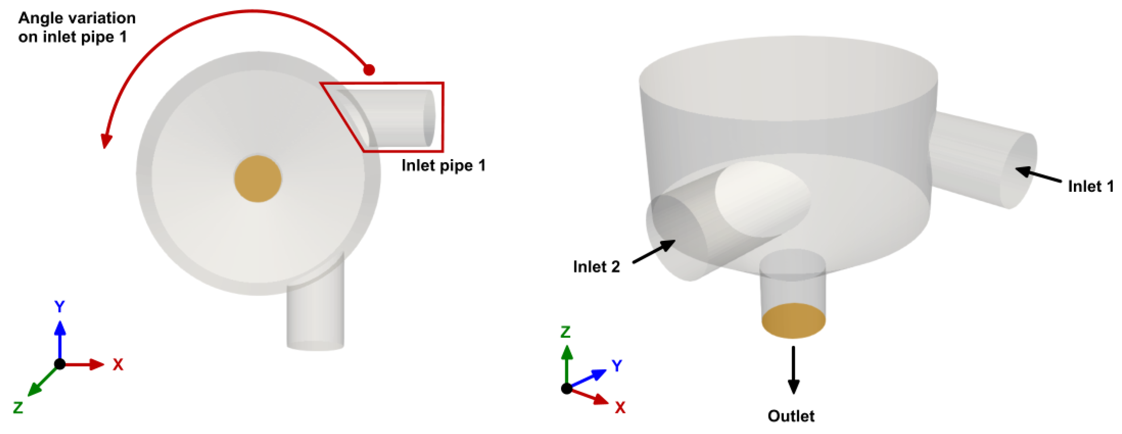
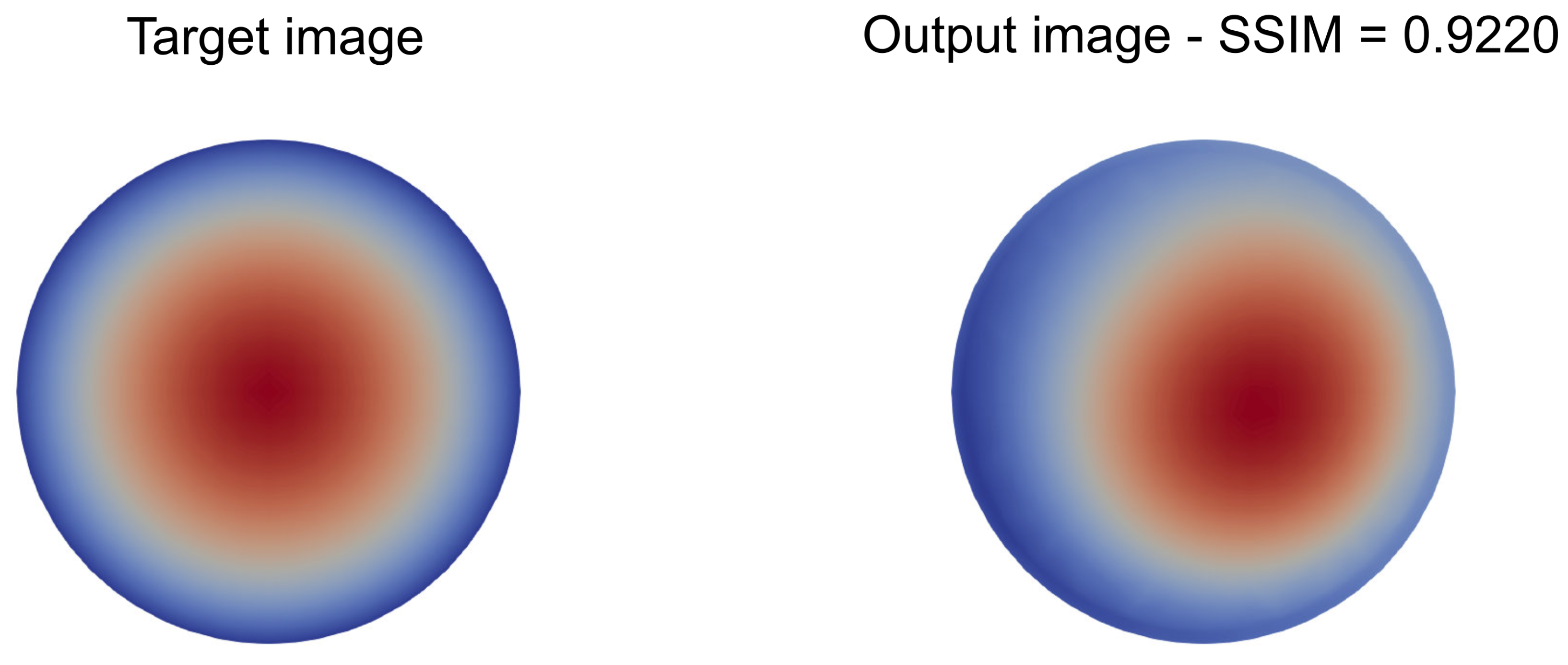
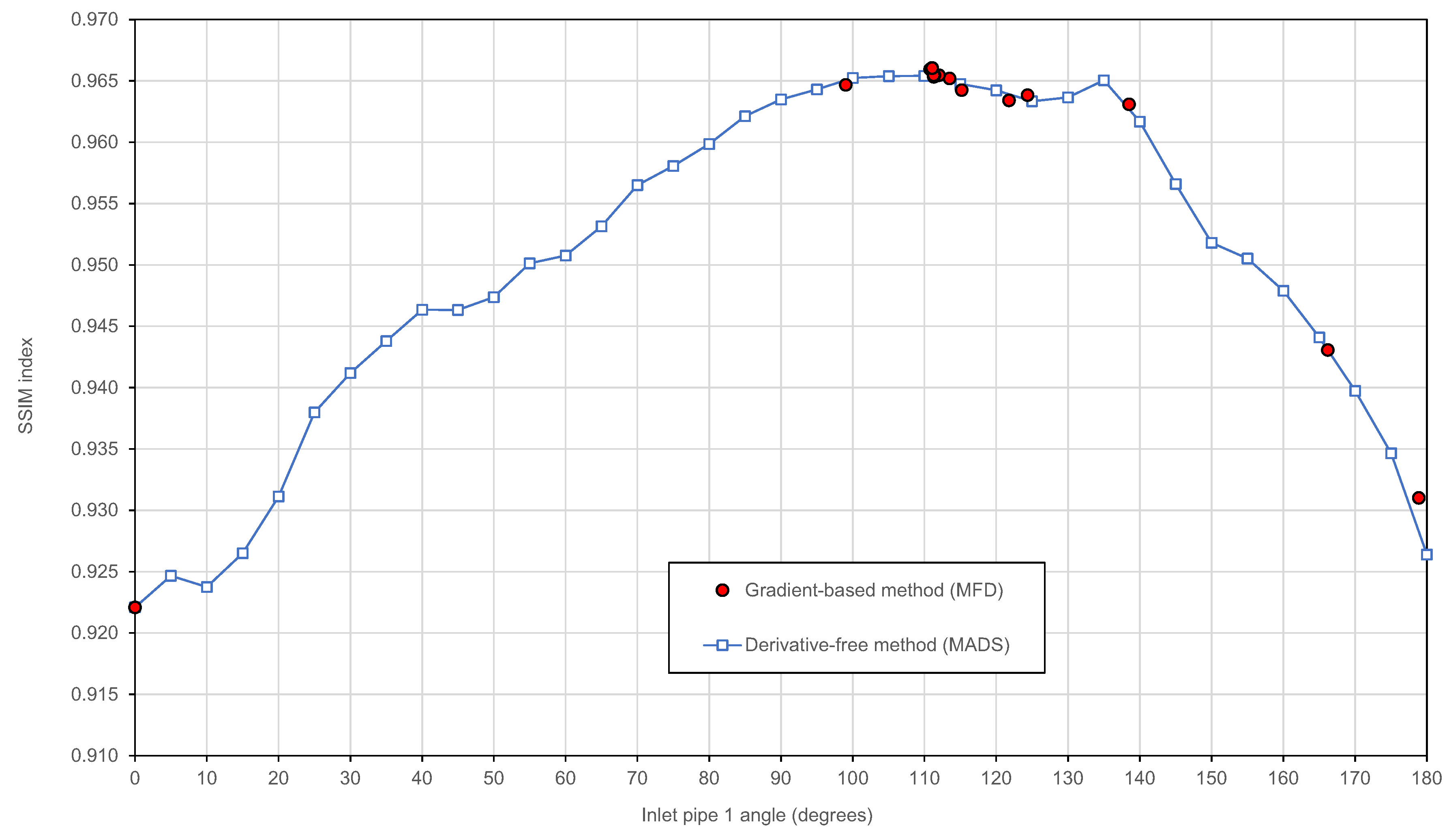
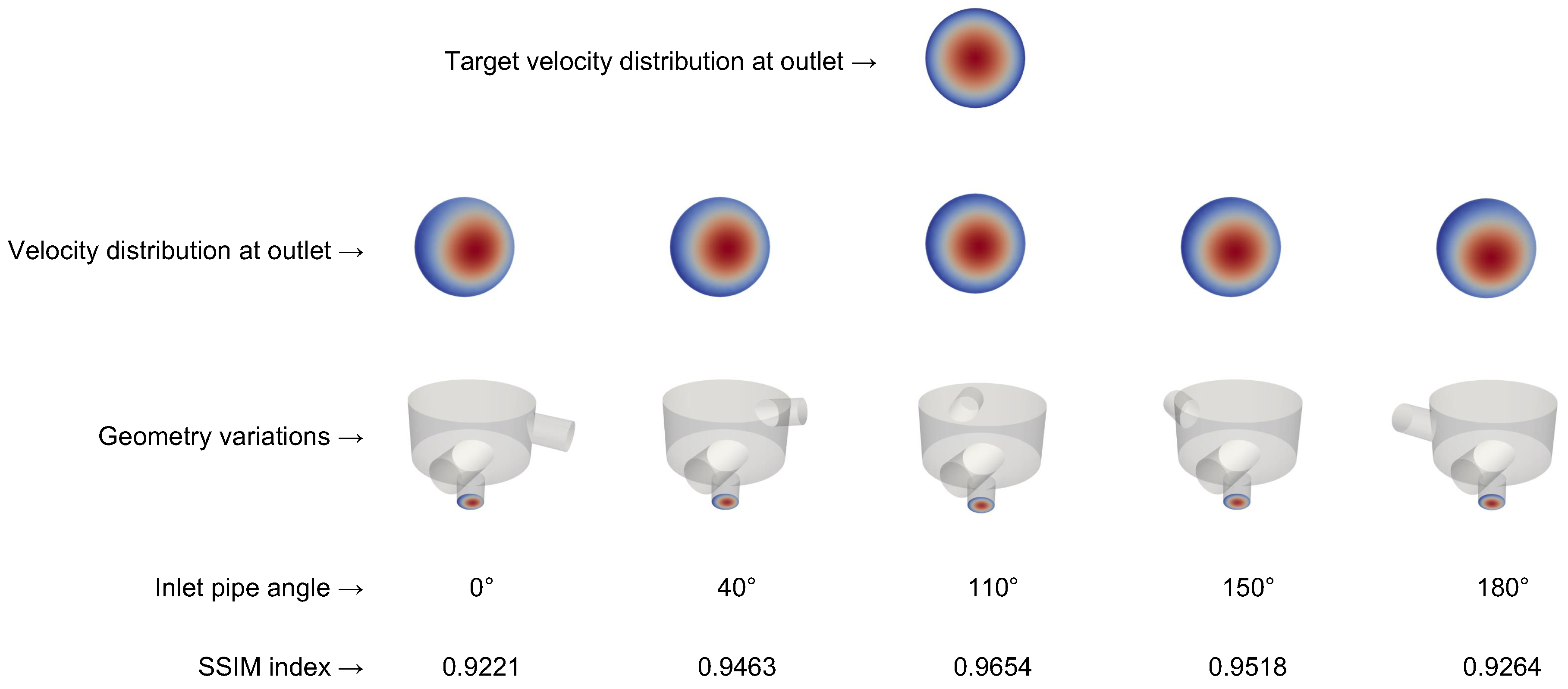
3.2. Static Mixer Optimization Case

In this case, we introduce the use of a qualitative metric to conduct the engineering design study. We also compare the outcome of a DO study and a DSE study. The geometry used in this case is shown in Figure 7, and it corresponds to a static mixer with two inlets and one output. The goal, in this case, is to obtain a given velocity distribution at the outlet by changing the angle of the inlet pipe 1 (refer to Figure 7). The velocity distribution field at the outlet was designed in such a way that the velocity normal to the outlet surface has a paraboloid distribution. Then, by using the SSIM index method (refer to Appendix A for an explanation), we compared the target image and the image of the current configuration (refer to Figure 8). The closer the SSIM index is to one, the more similar the images are; therefore, we aim at maximizing the QoI.

The simulations were conducted using OpenFOAM (version 7.0) [17,18]. To find the approximate solution of the governing equations, the SIMPLE pressure-velocity coupling method was used, together with the $k-epsilon$ turbulence model with wall functions, and a second-order accurate and stable discretization method for the convective, diffusive, and gradient terms. The Onshape document with all the dimensions is available at the following link (https://cad.onshape.com/documents/8f1312fafb3aac0f7bd3ed38/w/72a43b7cd8ca686e908ef122/e/33c606cd59a53e2b8532a94a).

The case setup is similar to the one presented in Section 3.1. The main difference is that we are introducing a new black-box application that requires additional steps so that it can be used inside the engineering design loop. The workflow specific to the data exchange between Dakota and the black-box solver (OpenFOAM in this case), is depicted in Figure 9 and discussed below. It is worth mentioning that the workflow is similar for different black-box applications, the only difference is in the formatting of the input and output files, and the data structure.

First, the Dakota input file is setup to reflect the number, range, and name of the design variables (parametrical variables), the number of QoI, and the objective of the optimization study (minimize or maximize). In the same input file, the optimization method or design space method is chosen, along with the required options. Also, sequential or asynchronous function evaluations can be chosen according to the resources available. Then, as depicted in Figure 9, a Template directory is created to store the parametrical input files, i.e., subject to change as a result of the optimization process (e.g., files containing the definition of the geometry, boundary conditions for inlet velocity, physical properties, etc.). The automatic update of the parametrical files located in the Template directory is done automatically by using a Dakota supplied utility or user-defined scripts. These utilities skim all files located in the Template directory and automatically insert the values generated by Dakota during the design optimization or the design exploration study, into the predefined locations in the template files. In this workflow, a Base case directory is also created, where all the files needed to update the geometry and to run the OpenFOAM simulations are stored. The simulation control script file (or simulation driver), denoted by the Control script box in Figure 9, merges the automatically edited files in the Template directory with the Base case directory, creating in this way a working directory for a specific set of design parameters. At this point, the control script executes all the steps related to the simulation, i.e., geometry update, meshing, and launching the solver (in serial or parallel). Finally, all the data generated is automatically post-processed following the instructions defined in the control script. This includes quantitative and qualitative post-processing, as well as data formatting. It should be emphasized that the Template directory and Base case directory are created by the user. Also, the automatic update of the parametrical files is done after merging the directories Template directory and Base case directory into a separate working directory. For the interested reader, the working case setup can be found at this link (https://github.com/joelguerrero/cloud-based-cad-paper/tree/master/static_mixer).

In Figure 10, we plot the outcome of the DO study using a gradient-based method (method of feasible directions or MFD [34,35] with numerical gradients computed using forward differences), and the DSE study using a uniform sampling for the inlet pipe angle (from 0 to 180 degrees). For the DO case, we used as starting point 0 degrees, and the case converged to the optimal value (pipe angle equal to 111.0549 degrees and SSIM index equal to 0.9660) in 31 function evaluations. In the DSE case, we explored the design space from 0 to 180 degrees, in steps of 5 degrees, so roughly speaking, we used the same number of function evaluations as for the DO case. From Figure 10, we can demonstrate that the DSE study, while not formerly converging to the optimal solution, gives more information about the design space than the DO method. From the DSE results, we can see that there is a plateau of the SSIM value for pipe angle values between 90 and 135 degrees. This information is not available when conducting DO studies, as the goal of these methods is to convergence to the optimal solution in an iterative fashion, and in doing so, some areas of the design space may remain unexplored. Using the data of the DSE study, we can also get a good estimate of the maximum value of the SSIM index, or we can use the data to construct a meta-model, and then use any DO method to find the optimal value. Both methods, DO and DSE, have their advantages and drawbacks and often is a good practice to use a combination of both, i.e., we first explore the design space in an inexpensive way, and then we use the information gathered from the DSE study to start a refined DO study.

In Figure 11, we show the velocity distribution at the outlet surface for five cases of the DSE study. In this figure, we also show the SSIM index value, the geometry layout, and the target image. As previously stated, the goal of this study was to obtain a given velocity distribution at the outlet (target image) by changing the angle of the inlet pipe. Then, by using the SSIM index method (Appendix A), we compare the target image and the image of the current configurations (as shown in Figure 11). The closer the SSIM index is to one, the more similar the images are. We highlight that we are using a qualitative metric instead of the traditional quantitative metrics used in engineering design studies. We designed beforehand the desired appearance of the field at the outlet, and then, by comparing the images in the design loop, we found the best match for our qualitative metric.

Again, we stress the fact that the loop is fully automatic and fault-tolerant, and it can be run concurrently and on the cloud. For the DSE case, we run eight simulations concurrently, each one using four cores. For the DO case, we were limited by the number of derivatives that can be computed at the same time. As this case only has one design variable, only one derivative can be computed. Therefore, the maximum number of concurrent simulations achievable in this DO case was two (one function evaluation and one gradient evaluation using forward differences), and each concurrent evaluation was conducted using eight cores.

Let us now conduct a DSE study using three design variables, namely the diameter of the inlet pipe one, the diameter of the inlet pipe two, and the angle of the inlet pipe one. Again, all the parametrical variables were defined in the Onshape’s document and modified using the Python API. This study was conducted using 170 experiments, generated using the space filling Latin hypercube sampling method (LHS) [2]. The simulations were run concurrently (eight simulations at the same time), and each simulation was run in parallel using four cores.

In Figure 12, we show another way to visualize high-dimensional data by using the parallel coordinates plot [43]. This kind of plot is extremely useful when visualizing and analyzing multivariate data, as it lets us identify how all variables are related. The highlighted line in Figure 12 represents the best solution (maximum SSIM index value), and shows the respective values of the design variables. In this DSE case, we can see that solutions that are better than the solution obtained using one design variable (SSIM = 0.9660), can be obtained by also changing the diameters of the inlet pipes. These solutions are shown in Figure 13. It worth mentioning that the parallel coordinates plots implemented are interactive; this allows us to isolate a range of values in real time. We can even change the order of the columns interactively and compare the slopes between variables. The scripts used for the parallel coordinates plots, as well as the data, are available at the following link (https://github.com/joelguerrero/cloud-based-cad-paper/tree/master/parallel_coordinates_dse_case). The interactive parallel coordinates plot can be accessed at the following link (http://joelguerrero.github.io/parallel_coordinates_dse_case/).

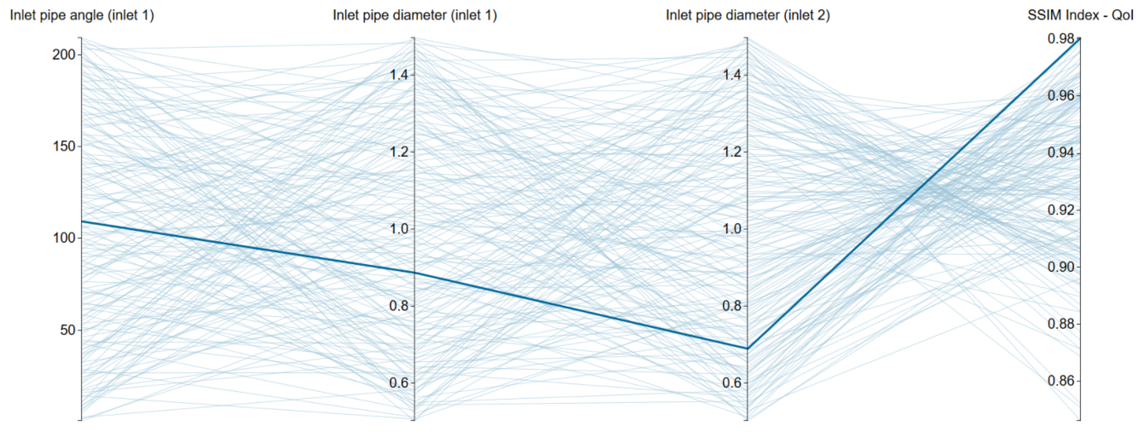
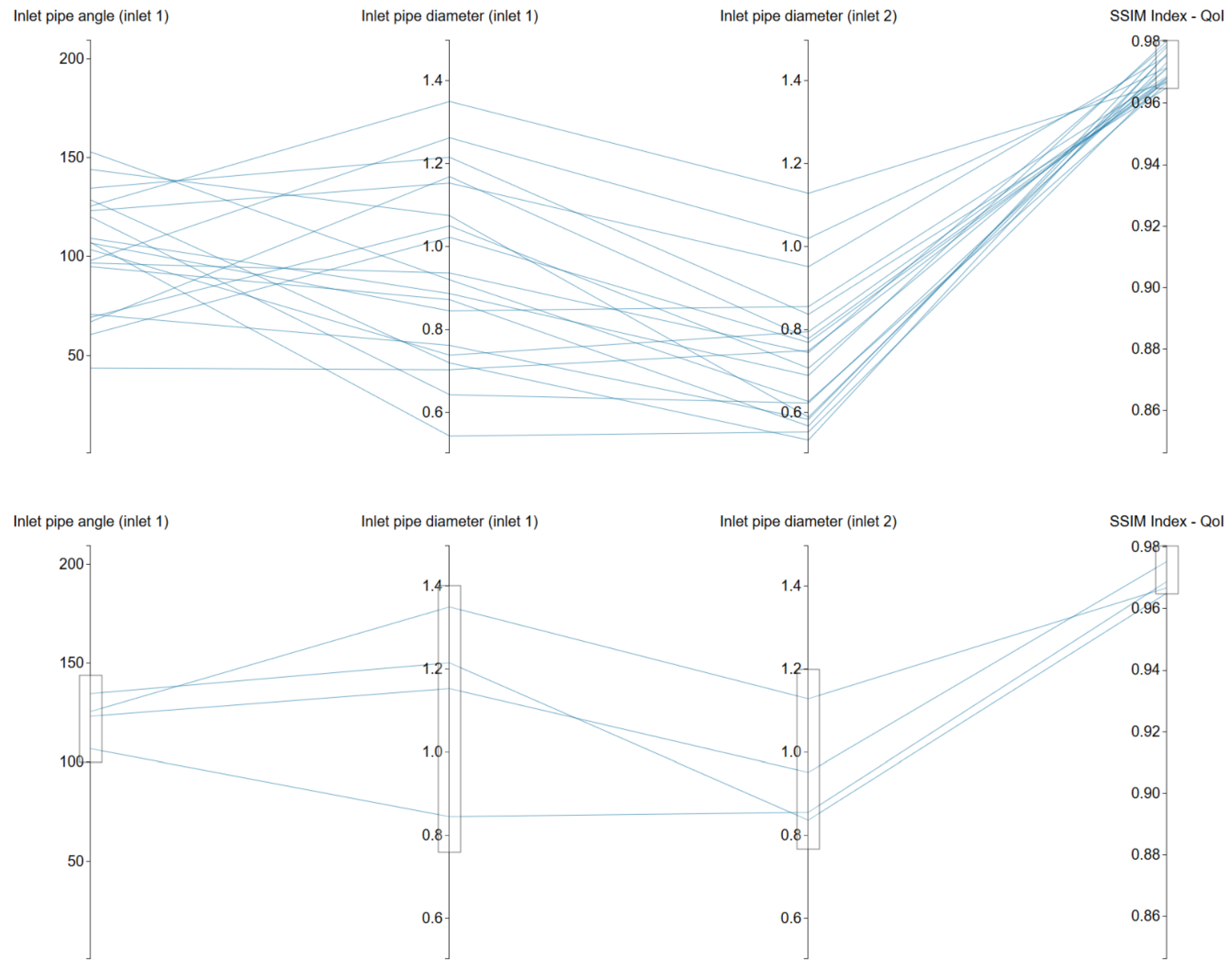
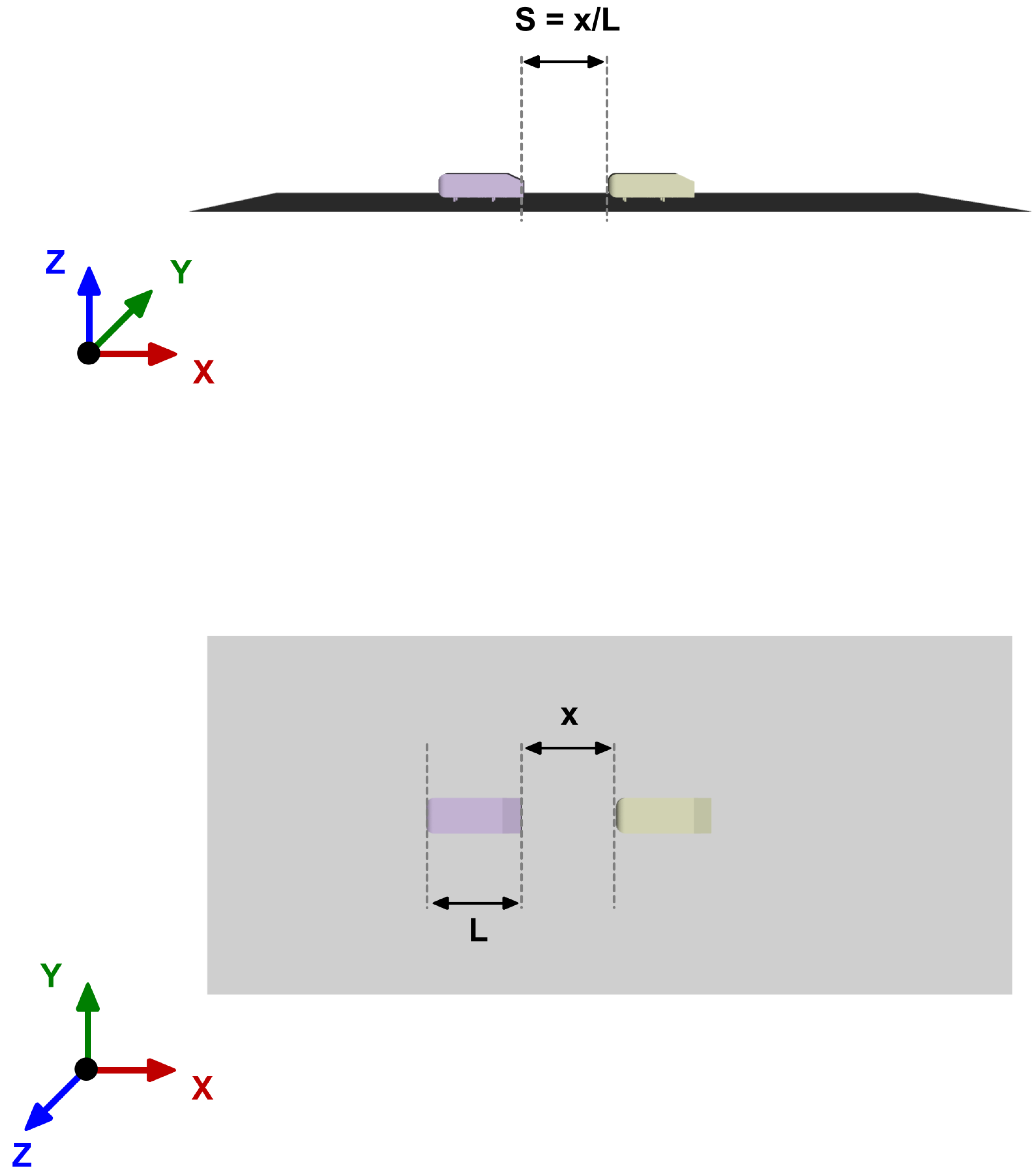
3.3. Two Ahmed Bodies in Platoon

In this case, we use the engineering design loop to conduct a parametric study. We compare the numerical results obtained with the current framework, against the experimental results obtained in references [44,45]; therefore, this is also a validation case. The simulations were conducted using OpenFOAM (version 7.0) [17,18]. To find the approximate solution of the governing equations, the SIMPLE pressure-velocity coupling method was used, together with the $k-\omega$ SST turbulence model with wall functions, and a second-order accurate and stable discretization method for the convective, diffusive, and gradient terms.

The study was conducted at different inter-vehicle spacing, an Ahmed body slant angle equal to 25 degrees, and an inlet velocity equal to 40 m/s. The QoI to measure is the normalized drag in platooning. In Figure 14, we depict a sketch of the computational domain and the definition of the inter-vehicle spacing S. From the parametrization used when creating the solid model, the two Ahmed bodies can be simulated in any formation with different slant angles, where everything can be controlled using configuration variables. The Onshape document with all the dimensions is available at the following link (https://cad.onshape.com/documents/b691f01f6fadba22433180ad/w/28165b21b45b4fee07e761b8/e/93c2ec3a1d01f9149d0557b1).

In Figure 15, we plot the outcome of this parametric study, where the normalized drag coefficient in platooning is computed as follows,

$$\begin{array}{c}\hfill C_{D_{Platooning}}={\displaystyle \frac{C_{D1}}{C_{D2}}}\end{array}$$

(9)

in this equation, $C_{D1}$ is the drag coefficient of the Ahmed body in a platoon position (front, back, sideways, or any combination), and $C_{D2}$ is the drag coefficient of the single Ahmed body. From the results presented in Figure 15, it can be observed a satisfactory agreement between the numerical and experimental values. It is worth mentioning that the simulations were run concurrently (four simulations at the same time), and each simulation was run in parallel using six cores.

In this final application, we only conducted a parametrical study with one design variable. However, this study served to demonstrate the usability of the framework for complex validation cases. The reader should be aware that this case can be extended to more complex scenarios; for example, we could simulate one Ahmed body overtaking the other one.

4. Conclusions and Future Perspectives

In this manuscript, we presented an engineering design framework to perform design optimization and design space exploration studies. The engineering design loop implemented, allows for sequential and concurrent simulations (i.e., many simulations can be run at the same time), and each simulation can be run in parallel; this allows reduction of the output time of the design loop considerably. The optimization loop is fault-tolerant and software agnostic, and it can be interfaced with any application able to interact using input/output files via a command-line interface. The code coupling capabilities were provided by the library Dakota, and all the tools used in this work are open-source and freeware.

Two novel features were introduced in the workflow. First, the use of a cloud-based parametric CAD tool that gives engineers and designers complete control over the geometry during the design loop. This feature allows users to deploy the design loop in any platform as the installation is not required. It also lets the designers interact with the parametric CAD model using a programmatic API. Introducing the CAD tool into the design loop has been traditionally a problem because most of the CAD applications run in Windows OS. In contrast, the simulation software runs in Unix-like OS. Furthermore, in traditional CAD tools is not possible to interact with the parametric model using a programmatic environment; they take all the inputs via a graphical user interface that cannot be controlled in an automatic design loop. The use of the cloud-based CAD tool allowed us to circumvent these problems.

Secondly, the use of the SSIM index method to drive the design study. By using this metric, it is possible to compare images instead of integral quantities. We can now design beforehand how the field will look like in a given location of the domain, and the design loop will try to find the best match for that qualitative metric.

From the numerical experiments presented, it was demonstrated the flexibility and usability of the proposed workflow to tackle engineering design problems using different approaches. As for the optimization strategy concerns, we used gradient-based methods, derivative-free methods, surrogate-based optimization, and design space exploration techniques. All the methods delivered satisfactory results. The SSIM index method also proved to be very robust and easy to implement.

This tool, together with reduced-order models and surrogate models, has the potential to open the door to generative design in CFD. We look forward to working in this field, together with machine learning techniques and more advanced image recognition algorithms.

References

1. Mattson, C.A. Design Exploration. Available online: https://design.byu.edu/blog/design-exploration-presentation-given-stanford-university-15-jan-2014 (accessed on 22 February 2020).
2. Forrester, A.; Sobester, A.; Keane, A. Engineering Design via Surrogate Modeling. A Practical Guide; Wiley: Hoboken, NJ, USA, 2008. [Google Scholar]
3. Guerrero, J.; Cominetti, A.; Pralits, J.; Villa, D. Surrogate-Based Optimization Using an Open-Source Framework: The Bulbous Bow Shape Optimization Case. Math. Comput. Appl. 2018, 23, 60. [Google Scholar] [CrossRef] [Green Version]
4. Romero, V.J.; Swiler, L.P.; Giunta, A.A. Construction of response surfaces based on progressive lattice-sampling experimental designs. Struct. Saf. 2004, 26, 201–219. [Google Scholar] [CrossRef]
5. Kochenderfer, M.; Wheeler, T. Algorithms for Optimization; MIT Press: Cambridge, MA, USA, 2019. [Google Scholar]
6. Gen, M.; Cheng, R. Genetic Algorithms and Engineering Optimization; Wiley-Interscience: Hoboken, NJ, USA, 2000. [Google Scholar]
7. Vanderplaats, G. Multidiscipline Design Optimization; Vanderplaats Research & Development, Inc.: Colorado Springs, CO, USA, 2007. [Google Scholar]
8. Papalambros, P.; Wilde, D. Principles of Optimal Design. Modeling and Computation; Cambridge University Press: Cambridge, UK, 2017. [Google Scholar]
9. Nocedal, J.; Wright, S. Numerical Optimization; Springer: Berlin/Heidelberg, Germany, 2006. [Google Scholar]
10. Chong, E.; Zak, S. An Introduction to Optimization; Wiley: Hoboken, NJ, USA, 2013. [Google Scholar]
11. Sobieszczanski-Sobieski, J.; Morris, A.; van Tooren, M.; Rocca, G.L.; Yao, W. Multidisciplinary Design Optimization Supported by Knowledge Based Engineering; Wiley: Hoboken, NJ, USA, 2015. [Google Scholar]
12. Chauhan, S.; Hwang, J.; Martins, J. An automated selection algorithm for nonlinear solvers in MDO. Struct. Multidiscip. Optim. 2018, 58, 349–377. [Google Scholar] [CrossRef] [Green Version]
13. Martins, J. The adjoint method in multidisciplinary design optimization—Special session in honor of Antony Jameson’s 85th birthday. In Proceedings of the AIAA SciTech Forum, Nashville, TN, USA, 6 January 2020. [Google Scholar]
14. Vassberg, J.C.; Jameson, A. Introduction to Optimization and Multidisciplinary Design Part I: Theoretical Background for Aerodynamic Shape Optimization; Lecture Series March 2016; Von Karman Institute: Brussels, Belgium, 2016. [Google Scholar]
15. Keane, A.J.; Nair, P.B. Computational Approaches for Aerospace Design: The Pursuit of Excellence; John Wiley & Sons: Hoboken, NJ, USA, 2005. [Google Scholar]
16. Martins, J.R.R.A.; Lambe, A.B. Multidisciplinary Design Optimization: A Survey of Architectures. AIAA J. 2013, 51, 2049–2075. [Google Scholar] [CrossRef] [Green Version]
17. The OpenFOAM Foundation. Available online: http://www.openfoam.org (accessed on 22 February 2020).
18. Weller, H.G.; Tabor, G.; Jasak, H.; Fureby, C. A tensorial approach to computational continuum mechanics using object-oriented techniques. Comput. Phys. 1998, 12, 620–631. [Google Scholar] [CrossRef]
19. Dakota Web Page. 2018. Available online: https://dakota.sandia.gov/ (accessed on 22 February 2020).
20. Adams, B.M.; Eldred, M.S.; Geraci, G.; Hooper, R.W.; Jakeman, J.D.; Maupin, K.A.; Monschke, J.A.; Rushdi, A.A.; Stephens, J.A.; Swiler, L.P.; et al. Dakota, a Multilevel Parallel Object-Oriented Framework for Design Optimization, Parameter Estimation, Uncertainty Quantification, and Sensitivity Analysis: Version 6.10 User Manual; Sandia National Laboratories: Albuquerque, NM, USA, 2019. [Google Scholar]
21. The Visualization Toolkit (VTK). Available online: http://www.vtk.org (accessed on 22 February 2020).
22. Onshape Product Development Platform. Available online: http://www.onshape.com (accessed on 22 February 2020).
23. Slotnick, J.; Khodadoust, A.; Alonso, J.; Darmofal, D.; Gropp, W.; Lurie, E.; Mavriplis, D. CFD Vision 2030 Study: A Path To Revolutionary Computational Aerosciences; Technical Report; NASA: Hampton, VA, USA, 2014.
24. Daymo, E.; Tonkovich, A.L.; Hettel, M.; Guerrero, J. Accelerating reactor development with accessible simulation and automated optimization tools. Chem. Eng. Process. Process Intensif. 2019, 142, 107582. [Google Scholar] [CrossRef]
25. Xia, C.C.; Gou, Y.J.; Li, S.H.; Chen, W.F.; Shao, C. An Automatic Aerodynamic Shape Optimisation Framework Based on DAKOTA. IOP Conf. Ser. Mater. Sci. Eng. 2018, 408, 012021. [Google Scholar] [CrossRef]
26. Byrne, J.; Cardiff, P.; Brabazon, A.; O’Neill, M. Evolving parametric aircraft models for design exploration. J. Neurocomput. 2014, 142, 39–47. [Google Scholar] [CrossRef]
27. Ohm, A.; Tetursson, H. Automated CFD Optimization of a Small Hydro Turbine for Water Distribution Networks; Technical Report; Chalmers University of Technology: Göteborg, Sweden, 2017. [Google Scholar]
28. Sousa, J.; Gorlé, C. Computational urban flow predictions with Bayesian inference: Validation with field data. Build. Environ. 2019, 154, 13–22. [Google Scholar] [CrossRef]
29. Kiani, H.; Karimi, F.; Labbafi, M.; Fathi, M. A novel inverse numerical modeling method for the estimation of water and salt mass transfer coefficients during ultrasonic assisted-osmotic dehydration of cucumber cubes. Ultrason. Sonochem. 2018, 44, 171–176. [Google Scholar] [CrossRef]
30. Habla, F.; Fernandes, C.; Maier, M.; Densky, L.; Ferras, L.; Rajkumar, A.; Carneiro, O.; Hinrichsen, O.; Nobrega, J.M. Development and validation of a model for the temperature distribution in the extrusion calibration stage. Appl. Therm. Eng. 2016, 100, 538–552. [Google Scholar] [CrossRef]
31. Khamlaj, T.A.; Rumpfkeil, M.P. Analysis and optimization of ducted wind turbines. Energy 2018, 162, 1234–1252. [Google Scholar] [CrossRef]
32. Montoya, M.C.; Nieto, F.; Hernandez, S.; Kusano, I.; Alvarez, A.; Jurado, J. CFD-based aeroelastic characterization of streamlined bridge deck cross-sections subject to shape modifications using surrogate models. J. Wind Eng. Ind. Aerodyn. 2018, 177, 405–428. [Google Scholar] [CrossRef]
33. Kelm, S.; Müller, H.; Hundhausen, A.; Druska, C.; Kuhr, A.; Allelein, H.J. Development of a multi-dimensional wall-function approach for wall condensation. Nucl. Eng. Des. 2019, 353, 110239. [Google Scholar] [CrossRef]
34. Zoutendijk, G. Methods of Feasible Directions: A Study in Linear and Non-Linear Programming; Elsevier: Amsterdam, The Netherlands, 1960. [Google Scholar]
35. Vanderplaats, G.N. An efficient feasible directions algorithm for design synthesis. AIAA J. 1984, 22, 1633–1640. [Google Scholar] [CrossRef]
36. Le Digabel, S. Algorithm 909: NOMAD: Nonlinear Optimization with the MADS Algorithm. ACM Trans. Math. Softw. 2011, 37. [Google Scholar] [CrossRef]
37. Guerrero, J. Opportunities and challenges in CFD optimization: Open Source technology and the Cloud. In Proceedings of the Sixth Symposium on OpenFOAM® in Wind Energy (SOWE), Göteborg, Sweden, 13–14 June 2018. [Google Scholar]
38. Oliver, M.; Webster, R. Kriging: A Method of Interpolation for Geographical Information Systems. Int. J. Geogr. Inf. Syst. 1990, 4, 313–332. [Google Scholar] [CrossRef]
39. Adams, B.M.; Eldred, M.S.; Geraci, G.; Hooper, R.W.; Jakeman, J.D.; Maupin, K.A.; Monschke, J.A.; Rushdi, A.A.; Stephens, J.A.; Swiler, L.P.; et al. Dakota, a Multilevel Parallel Object-Oriented Framework for Design Optimization, Parameter Estimation, Uncertainty Quantification, and Sensitivity Analysis: Version 6.10 Theory Manual; Sandia National Laboratories: Albuquerque, NM, USA, 2014.
40. Dalbey, K.R.; Giunta, A.A.; Richards, M.D.; Cyr, E.C.; Swiler, L.P.; Brown, S.L.; Eldred, M.S.; Adams, B.M. Surfpack User’s Manual Version 1.1; Sandia National Laboratories: Albuquerque, NM, USA, 2013.
41. Dalbey, K.R. Efficient and Robust Gradient Enhanced Kriging Emulators; Technical Report; Sandia National Laboratories: Albuquerque, NM, USA, 2013.
42. Giunta, A.A.; Watson, L. A comparison of approximation modeling techniques: Polynomial versus interpolating models. In 7th AIAA/USAF/NASA/ISSMO Symposium on Multidisciplinary Analysis and Optimization; NASA Langley Technical Report Server: Hampton, VA, USA, 1998. [Google Scholar]
43. Inselberg, A. Parallel Coordinates, Visual Multidimensional Geometry and Its Applications; Springer: Berlin/Heidelberg, Germany, 2009. [Google Scholar]
44. Pagliarella, R.M.; Watkins, S.; Tempia, A. Aerodynamic Performance of Vehicles in Platoons: The Influence of Backlight Angles. SAE World Congr. Exhib. SAE Int. 2007. [Google Scholar] [CrossRef]
45. Pagliarella, R.M. On the Aerodynamic Performance of Automotive Vehicle Platoons Featuring Pre and Post-Critical Leading Forms; Technical Report; RMIT University: Melbourne, Austrialia, 2009. [Google Scholar]
46. Sampat, M.P.; Wang, Z.; Gupta, S.; Bovik, A.C.; Markey, M.K. Complex wavelet structural similarity: A new image similarity index. IEEE Trans. Image Process. 2009, 18, 2385–2401. [Google Scholar] [CrossRef]
47. Wang, Z.; Bovik, A.C.; Sheikh, H.R.; Simoncelli, E.P. Image Quality Assessment: From Error Visibility to Structural Similarity. IEEE Trans. Image Process. 2004, 13, 600–612. [Google Scholar] [CrossRef] [Green Version]
48. Eskicioglu, A.M.; Fisher, P.S. Image Quality Measures and Their Performance. IEEE Trans. Commun. 1995, 43, 2959–2965. [Google Scholar] [CrossRef] [Green Version]
49. Ndajah, P.; Kikuchi, H.; Yukawa, M.; Watanabe, H.; Muramatsu, S. SSIM image quality metric for denoised images. In Proceedings of the International Conference on Visualization, Imaging and Simulation, Faro, Portugal, 3–5 November 2010; pp. 53–57. [Google Scholar]
50. Lin, Y.; Chai, L.; Zhang, J.; Zhou, X. On-line burning state recognition for sintering process using SSIM index of flame images. In Proceedings of the 11th World Congress on Intelligent Control and Automation, Shenyang, China, 29 June–4 July 2014; pp. 2352–2357. [Google Scholar] [CrossRef]
51. Priyal, S.P.; Bora, P.K. A study on static hand gesture recognition using moments. In Proceedings of the International Conference on Signal Processing and Communications (SPCOM), Bangalore, India, 18–21 July 2010; pp. 1–5. [Google Scholar] [CrossRef]
52. Van der Walt, S.; Schönberger, J.L.; Nunez-Iglesias, J.; Boulogne, F.; Warner, J.D.; Yager, N.; Gouillart, E.; Yu, T. Scikit-image: Image processing in Python. PeerJ 2014, 2, e453. [Google Scholar] [CrossRef]
Figure 1. Graphical summary of the engineering design loop.
Fluids 05 00036 g001
Figure 2. Workflow of the problem setup using the proposed cloud-based framework.
Fluids 05 00036 g002
Figure 3. Definition of configuration variables and measurements in the Onshape document.
Fluids 05 00036 g003
Figure 4. Onshape’s cloud-based client-server communication using RESTful API. The client communicates with Onshape’s server using Python API keys and OAuth authentication.
Fluids 05 00036 g004
Figure 5. Scatter plot matrix of the cylinder optimization case using two design variables. In the upper triangular part of the plot, the Spearman correlation is shown. In the diagonal of the matrix, the histograms showing the data distribution are displayed. In the lower triangular part of the matrix, the data distribution is shown using scatter plots. In the last row of the matrix plot, the response of the QoI in function of the design variables and the non-linear (NL) constraint is illustrated, together with a quadratic regression model.
Fluids 05 00036 g005
Figure 6. Left image: contour plot of the QoI (total surface). Right image: contour plot of the non-linear constraint (volume); in the image, the white line represents the range where the volume is 354 cm 3 < Volume < 356 cm 3 . In both images, the green circle represents the starting point, the red circle represents optimal value, the yellow circles represent the path followed by the optimization algorithm (note that the gradient evaluations are not plotted), and the white circles represent the sampling points.
Fluids 05 00036 g006
Figure 7. Static mixer geometry.
Fluids 05 00036 g007
Figure 8. Velocity distribution normal to the outlet surface. Left image: reference velocity distribution or target image. Right image: image of the velocity distribution for a non-optimal case. To determine if the images are similar, we used the SSIM index method. The closer the SSIM index of the output image is to one, the more similar the images are.
Fluids 05 00036 g008
Figure 9. Workflow for data exchange between Dakota and OpenFOAM. The white rectangles denote process blocks, light-shaded blue document symbols denote unchanging sets of files, and light-shaded green document symbols indicate files that change with each set of design parameters generated by Dakota or after the end of the evaluation of the QoI. The light-shaded grey area denotes the domain of the control script that automatically prepares the case; this includes, CAD geometry, mesh generation, launching the solver, quantitative and qualitative post-processing, and automatic formatting of input and output files.
Fluids 05 00036 g009
Figure 10. Comparison of the outcome of the DO and DSE studies. The QoI used was the SSIM index.
Fluids 05 00036 g010
Figure 11. Qualitative comparison of the velocity distribution at the outlet. The SSIM method was used to compare the images. In the SSIM method, a value of 1 means that the images are identical. The target image is shown in the first row of the figure.
Fluids 05 00036 g011
Figure 12. Parallel coordinates plot of the outcome of the DSE study using three design variables. The highlighted line represents the best solution.
Fluids 05 00036 g012
Figure 13. Parallel coordinates plot with filters. In the top image, the QoI has been filtered ( 0.9660 S S I M 1 ). In the bottom figure, we apply additional filters to the design variables.
Fluids 05 00036 g013
Figure 14. Spacing definition of the two Ahmed bodies, where x is the distance between the two bodies, L is the Ahmed body length, and S is the non-dimensional inter-vehicle spacing ( S = x / L ).
Fluids 05 00036 g014
Figure 15. Normalized drag coefficient against inter-vehicle spacing S. The continuous lines represent the numerical results. The experimental results (dashed line) were taken from references [44,45].
Fluids 05 00036 g015