Numerical Study on the Flow and Heat Transfer Coupled in a Rectangular Mini-Channel by Finite Element Method for Industrial Micro-Cooling Technologies

Abstract

Nowadays, cooling high thermal flows in compact volumes continues to be one of the crucial problems in the industry. With the advent of advanced technologies, much more attention has been paid to how to improve the performance of cooling systems in the area of micro-technologies. Rectangular mini-channels are typical representatives which commonly used for cooling applications. However, micro-technologies still face the problem of low performance due to the low productivity of cooling related to unbefitting physical parameter values. Here, this work studies the applicability of the heat transfer scheme of convective flow and flow boiling in a rectangular mini-channel for satisfying the cooling requirement of industrial micro-technologies, through a simulation model governed by the coupled mechanism from Navier-Stokes (N-S) equation and heat transfer equations with phase change effect. In this work, various hydraulic diameters and different inlet fluid speed are used to calculate the different velocity profiles, pressure drops, coefficients of friction and finally, the distribution of the temperatures and dissipated heat flux. The simulation results show the applicability of the rectangular mini-channel in diverse applications such as engine cooling, electronic components, automotive on-board electronics and aerospace engineering. Flow boiling simulation results reveal that the obtained patterns were smooth mixture flow and discrete flow. The dissipated heat flux can reach 1.02–5.34 MW/m² for a hydraulic diameter of 0.5 mm. We show that the system with the gradient temperature that evolves increasingly along the top and bottom walls of the channels presents the highest heat flux dissipated in flow boiling. Additionally, the fin efficiency of the system is 0.88 and the coefficient value of convective heat transfer is in the range between 5000 < h < 100,000, which indicates the flow boiling heat transfer is effective in the mini-channel when the Reynolds number is less than 400. It provides a significant heat exchange for cooling in these application areas.

1. Introduction

Microfluidics is the science and innovation of frameworks that manage the exact control of fluids with small amounts of tiny scales in microchannels. Microfluidics is viewed as a new area of choice for the control of liquids in channels of several micrometers [1]. The smaller scale was usually claimed, which implies the accompanying attributes—small volumes (“L, nL, pL, fL”) and small size leading to low energy consumption and special micro-domain effects [2]. So, microfluidics benefits in several aspects and it usually involves microstructures with a much-reduced size of a geometry. Microstructures nowadays pose specific problems during the modeling and the optimization because of their reduced dimensions. The qualities of small-scale streams, called microfluidics, in the micrometric scales are marginally not quite the same as the perceptible streams. Many physical phenomena can no longer be neglected in microchannels with macroscopic scale. That happens because the area/volume ratio is much higher in these microsystems. This increase substantially affects the flows of mass, momentum and energy through the surfaces and, in particular, the fluid-fluid, fluid-wall interfaces. The importance of boundary conditions and particularly surface conditions, is significantly increased.

Nowadays, the development of power electronics, consumer electronics and miniaturized mechanical and energy systems face some difficulties for improving the cooling effect when the high temperatures in compact volumes are involved. To ensure proper operation at optimum temperatures, advanced heat transfer methods must be used to overcome such difficulties by developing efficient and reliable heat rejection means [3]. Thus, one of the proposed techniques is cooling using microchannels and mini-channels by a single or two-phase flow because it offers high performance in heat transfer [4]. Therefore, the mini-channels and microchannels could meet the requirements of some cooling applications and they have been employed in diverse applications as follows—Biomedical engineering (chemical analyzes, injections and dosing of active products) [5]; Space engineering (micro-propulsion, micro pumping for fluid cooling loops) [6]; Electronic engineering (Component cooling) [7]; Automotive Engineering (Injection control in engines, miniature heat exchangers) [8]; MEMS “Micro Electro Mechanical Systems” (inkjet printing) [9]; and the conformal cooling system for injection molding technology [10,11].

Among the initial investigations in this field, it is still challenging to achieve a compact, high-performance forced liquid cooling of planar integrated circuits. The researchers realized that the convective heat transfer coefficient h between the substrate and the coolant could be the first factor to achieve low thermal resistance [12]. The friction factors were estimated for the flow of gases (N₂, H₂) in the fine channels utilized for the micro-miniature Joule-Thompson refrigerators [13]. Their measured friction factor was higher than the theoretical predictions. The flow of water and various biological fluids through microchannels etched on silicon and covered with a glass plate has been analyzed [14,15,16]. Their channels had a trapezoidal cross-section and differed from 50 to 150 µm in width and from 20 to 40 µm in depth. The results showed an increase in the coefficient of friction of almost 50% compared to the theoretical values. The estimation of refrigerant R-12 pressure loss was taken in a single or few smaller-scale channels [17]. The hydraulic diameters utilized in their work were 2.64 mm for the first and 1.56 mm for the second. The recommendation of the elements of the microstructures as indicated by their breadth D of the channels was made—Conventional channels whose diameter D_h ≥ 3 mm, mini-channels whose diameter D_h varies from 200 µm to 3 mm and microchannels whose diameter D_h is between 10 µm and 200 µm [18]. The friction factor measurements were presented in mini-channels varying from 1.13 mm to 300 µm in height, 60 mm in width and 150 mm in length, taken from a differential pressure sensor [19]. The results of the friction factor were above 14% to 50% larger than the predictions of conventional laminar laws, especially for small hydraulic diameters. The experimental studies on forced convective heat transfer and water flow characteristics in rectangular microchannels have been conducted with hydraulic diameters between 133 and 367 µm [20,21,22]. They showed the hydraulic diameters influence the heat transfer and the shape of the cross-section of channels does not influence the flow regimes for heat transfer. Therefore, they found that the thermal transfer in the laminar regime depends on the ratio of hydraulic diameter to the distance separating the microchannels. Moreover, the wall velocity slip decreases the hydraulic resistance and increases the convective heat transfer of laminar flow in a microchannel network [23]. In order to reach a minimum fluidic resistance, the optimized structure of the tree-like branching microchannel network was studied for the electroosmotic flow [24].

The increase in operating hours and the explosion of miniaturization projects created numerous problems due to the considerable increase in the heat flux generated by the electronic components. If the heat has not been dissipated in due time, there would be a problem with overheating. Hence the thermal control became progressively complex [25]. For these devices to provide reliable performance and not to be destroyed by the heat they generated, it was necessary to evacuate the thermal power very effectively to maintain an optimum operating temperature. Flow boiling in microchannels is getting important in several applications and has been widely examined as a cooling alternative because of its ability to generate high heat flux transfer. Thus, the study of the characteristics of flow boiling patterns in the rectangular mini-channel is necessary to understand the phase change mechanisms better. Therefore, numerous numerical studies were conducted to understand the phenomena that occur during the flow boiling process. The experimental results of water boiling in a single rectangular microchannel with a hydraulic diameter of 0.56 mm and a length of 62 mm proved that the important flow patterns were bubbly, slug, churn and annular flow [26]. Other investigation on the flow boiling of water in microchannels with a hydraulic diameter of 0.333 mm demonstrated that the observed flow patterns were bubbly flow, plug flow, churn flow and annular flow [27]. Some experimental data showed the gravitational orientation affected the flow patterns transitions [28]. Flow boiling heat transfer in an array with a hydraulic diameter varying from 0.1 to 0.54 mm was also investigated and it was found that the heat transfer coefficient was almost independent with heat flux at high heat flux [29].In the previous work, it has not been specified how to determine the exact area of application of the rectangular mini-channels by setting or adjusting the values of the parameters of velocity, pressure drop, coefficient of friction and phase transition and heat transfer flux. The simulations on heat transfer in mini-channel usually did not consider the gradient temperature boundary and the transient phase transition simultaneously.

Here, this study chooses a representative mini-channel with a rectangular cross-section as the basic elemental geometry for cooling structures and simulate the velocities profiles, drop pressures and friction factor and steady and transient heat transfers in the simplified singe-phase flow and more accurate two-phase (liquid and vapor) flow models of the fluidic flow through the mini-channel in different application areas. Modeling the coupled effect of the flow and heat transfer in a basic rectangular mini-channel with the consideration of phase change has been performed to better understand these different physical phenomena and to show how to determine the applicability of the rectangular mini-channel in certain industrial areas, through a depth study of heat transfer. The relationship between the relevance of the Reynolds number of the friction factor and dissipated heat flux has also been examined. Further, different boundary conditions of temperature gradients along the top and bottom walls of the min-channel were implemented. The results show the temperature gradient evolving progressively along the top and bottom of the channel leads to a high heat flux dissipated compared to that system with uniform temperature boundary. The simulation study on the heat transfer coupled with two-phase microflows accompanied with phase change presents the intrinsic laws of the heat transfer varying with flow characteristics, channel geometry, environmental temperature distribution along the rectangular mini-channels and help to understand better the flow boiling heat transfer process which occurs in rectangular mini-channel. We found that the observed flow boiling pattern are smooth mixture flow and discrete flow. The dissipated heat flux can reach 1.02–5.34 MW/m² for a hydraulic diameter of 0.5 mm and length 150 mm.

2. Materials and Methods

Table 1. Materials used in COMSOL Multiphysics.

Sections (Parts)	Materials
Walls	(1) No specific material, (2) Copper
Phase 1	Water, liquid
Phase 2	Water, gas

summarizes all the materials that were used in this simulation.

The comparison of the current state-of-the-art for heat transfer can be found in the supplementary in Section 1, Table S1.

The simplified geometric structure of this rectangular mini-channel in Figure 1 gives the dimensions—the channel length is 150 mm, the channel height is 4 mm and the hydraulic diameter ranging from 0.5 mm to 1 mm. Usually, the mini-channels used for heat transfer in the typical applications of electronic device or engine cooling needs at least an inlet connecter and an outlet connecter for practical controlling system. In the practices, the flow from inlet to outlet usually does not keep in a unified direction due to the requirement on compacting design and structure manufacture. Thus, the typical U-shaped structure was used.

2.1. Governing Equations

In fluid mechanics, Navier-Stokes equations are nonlinear partial differential equations that describe the motion of Newtonian fluids (hence gases and most liquids). In general, fluid flow in microchannels is laminar due to small channel dimensions. Reynold’s number, Re characterizes laminar flow within microfluidic devices, which is often much smaller than $2.3\times {10}^3$ according to the research work [30].

A computational fluids dynamics analysis was completed to explore the characteristics of fluid flow and heat transfer with the following assumptions—(1) the fluid is incompressible, (2) steady-state fluid flow and heat transfer, (3) The gravity effect is negligible in “mini-channels” when D_h ≤ 1 mm [31], radiation heat transfer and viscous dissipation are insignificant. Based on these assumptions, the Navier-Stokes (N-S) equations are the governing differential equations used to describe the fluid flow as follows [30]:

$$\rho \frac{\partial \overrightarrow{u}}{\partial t}=-\rho \overrightarrow{u}.\nabla \overrightarrow{u}+\mu {\nabla }^2\overrightarrow{u}-\nabla P+\overrightarrow{F}$$

(1)

$$\frac{\partial \overrightarrow{\rho }}{\partial t}+div\rho u=0,$$

(2)

where $\rho$ is the density of the fluid, $\overrightarrow{u}$ denotes the velocity vector of the fluid, $\mu$ is the dynamic viscosity of the liquid, $\nabla P$ is the pressure gradient and $\overrightarrow{F}$ is the external force applied to the fluid.

Besides, the following equations were employed in the phase-field method, which described the two-phase flow in phase initialization. To find the accurate location of the surface in this method, the Cahn-Hilliard equations (Navier-Stokes and continuity) were solved [32]:

$$\frac{\partial \varphi }{\partial t}+u·\nabla \varphi =\nabla ·\frac{{\gamma }^{\lambda }}{{\epsilon }_{pf}^2}\nabla \psi$$

(3)

$$\psi =-\nabla ·{\epsilon }_{pf}^2\nabla \varphi +({\varphi }^2-1)\varphi +\frac{{\epsilon }_{pf}^2}{\lambda }\left(\frac{\partial f}{\partial \varphi }\right),$$

(4)

where $\varphi =phipf$ is the dimensionless phase variable field, $\psi$ is the secondary phase field, $\gamma =\chi {\epsilon }_{pf}^2$ is the mobility, $\chi$ is the mobility tuning parameter in $m.s/kg$, ${\epsilon }_{pf}^{}$ is the parameter controlling interface thickness in m, $\lambda =3{\epsilon }_{pf}^2\sigma /\sqrt{8}$ is the mixing energy density. The volume fraction in the interface of the water (liquid) and the water (gas) are $V_{water,liquid}=\frac{1-\varphi }{2}$ and $V_{water,gas}=\frac{1+\varphi }{2}$ respectively. The density and the dynamic viscosity of the mixture of the two-phase model interface are defined throughout the interface accordingly:

$$\rho ={\rho }_w{V}_w+{\rho }_{gas}{V}_{gas}$$

(5)

$$\mu ={\mu }_w{V}_w+{\mu }_{gas}{V}_{gas}.$$

(6)

The surface tension considered as a body force applied is:

$$F_{st}=\left(\frac{\lambda }{{\epsilon }_{\mathrm{Pf}}^2}\psi -\frac{\partial f}{\partial \varphi }\right)\nabla \varphi +\left(\frac{{\left|\nabla \varphi \right|}^2}{2}+\frac{{\left({\varphi }^2-1\right)}^2}{4{\epsilon }_{P\mathrm{f}}^2}\right)\nabla \lambda -\left(\nabla \lambda ·\nabla \varphi \right)\nabla \varphi$$

(7)

The chemical potential G is expressed by the following equation referred to the phase-field variable and the parameter controlling interface thickness:

$$G=\lambda \left[-{\nabla }^2\varphi +\frac{\varphi ({\varphi }^2-1)}{{\epsilon }_{pf}^2}\right].$$

(8)

The heat transfer process is also governed by the equation of momentum, continuity equation aforementioned in equations 1 & 2 respectively and the equation of energy in the microchannel as given as [33].

Equation of energy conservation:

$$\frac{\partial }{\partial t}\left[\rho \left(e+\frac{1}{2}{u}^2\right)\right]+\nabla ·\left[\rho \mathbf{u}\left(e+\frac{1}{2}{u}^2\right)\right]=\nabla ·(k\nabla T)+\nabla ·\left(-p\mathbf{u}+\tau ·\mathbf{u}\right)+\mathbf{u}·\mathbf{F}+Q$$

(9)

where $\rho$, p, $\tau$, e, k, F, $u^2$, T, and $\mathbf{u}$ are the density, pressure, the viscous stress tensor, the internal energy per unit mass, thermal conductivity, the body force per unit mass, the square of velocity magnitude, the temperature, and fluid velocity vector respectively.

The flow of heat transferred to the fluid:

$$Q=q_m{C}_p(T_{out}-T_i{}_n),$$

(10)

where q_m is the mass flow of the fluid, T_out is the outlet temperature of the fluid and T_in is the inlet temperature.

In the module of heat transfer in fluids, the physical properties of the phase change material in fluid in phase initialization were governed by the following’s equations:

$$\rho ={\theta }_1{\rho }_1+{\theta }_2{\rho }_2$$

(11)

$$C_p=\frac{1}{\rho }({\theta }_1{\rho }_1{C}_{p,1}+{\theta }_2{\rho }_2{C}_{p,2})+L_{1\to 2}\frac{\partial {\alpha }_m}{\partial T},$$

(12)

with ${\theta }_1$ being the apparent dynamic contact angle of the fluid, ${\theta }_2$ the dynamic contact angle of the gas [34] and the total contact angle is ${\theta }_1+{\theta }_2=1$. The fraction of liquid phase, ${\alpha }_m=\frac{1}{2}\frac{{\theta }_2{\rho }_2-{\theta }_1{\rho }_1}{{\theta }_2{\rho }_2+{\theta }_1{\rho }_1}$, the thermal conductivity, $k={\theta }_1{k}_1+{\theta }_2{k}_2$ and k₁,k₂ the thermal conductivity of the fluid and the gas respectively.

The gravity is solved in phase initialization by this equation:

$$\rho (\mathbf{u}·\nabla )\mathbf{u}=\nabla ·\left[-p\mathrm{I} + \mathrm{K}\right]+\mathbf{F}+\rho \mathrm{g},$$

(13)

with g being the acceleration of the gravity, which is equal to 0 m/s² along with the horizontal position and I the identity matrix.

2.1.1. Laminar Flow

Laminar flow is defined by fluid flow along smooth paths in layers moving smoothly at low speed past adjacent layers with little or no mixing [35]. (Section 1.1, Figure S1 in Supplementary).

2.1.2. Law of Friction, Number of Theoretical Poiseuille

The coefficient of friction and the theoretical number of Poiseuille in single-phase flow (Section 1.2 in Supplementary) for the laminar flow through the rectangular channels was calculated using the polynomial type equation [36], which gives the exact solution with an accuracy of $\pm 5\%$:

$$c_f=\frac{24}{{\mathrm{Re}}_{Dh}}\left(1-1.3553·\alpha +1.9467·{\alpha }^2-1.7012·{\alpha }^3+0.9564·{\alpha }^4-0.2537·{\alpha }^5\right),$$

(14)

with $\alpha$ being the defined aspect ratio of the height to the width of the cross-section of the channel.

In two-phase flow, the friction factor was estimated by the correlation method [37]:

$${\xi }_{pred}={\left[-2\log \left(\frac{e}{3.7065d}-\frac{5.0452}{{\mathrm{Re}}^{\ast }}\log \left(\frac{1}{2.8257}{\left(\frac{e}{d}\right)}^{1.1098}+\frac{5.8506}{{\left({\mathrm{Re}}^{\ast }\right)}^{0.8981}}\right)\right)\right]}^{-2},$$

(15)

where ${\xi }_{pred}$ is the friction factor, e/d is the relative roughness.

2.2. Numerical Method

COMSOL Multiphysics is a finite element engineering science tool that allows entering coupled systems of partial differential equations to examine numerically and analyze the phenomenon Multiphysics. The equations described (1 and 2) are differential equations with nonlinear partial derivatives, elliptic and coupled. Owing to their complexity, these equations are solved, requiring a numerical method. There are three principal methods to formulate a continuous-discrete problem, finite difference method, finite element and finite volume. Each of these methods has applications depending upon the conditions of the geometry. The method used for this simulation in the COMSOL software is the finite element method (FEM). It is prevalent for the six advantages to this technique—modeling, adaptability, accuracy, time-dependent simulation, boundaries, visualization [38]. Significant distinctive problems of concern in fields include structural analysis, heat transfer, fluid flow, mass transport and electromagnetic potential.

2.2.1. Simulation Parameters

The inlet velocity is a key parameter in the determination of the flow regime. In COMSOL, the parametric sweep in the study was used to set the parameter values list at which the results could be plotted. Thus, the inlet velocities were defined as 0.5; 0.55; 0.6; 0.9; 1.1; 1.5; 1.8; 2.2 and 2.4 m/s.

Table 2. Parameters used in COMSOL.

Parameters	Value	Symbol
Inlet velocity	0.25 m/s	V1
Channel length	144 mm	L
Fluid density	1000 kg/m3	$\rho$
Viscosity dynamic	0.001 kg/m.s	$\mu$
Hydraulic diameters	0.5–0.98–1 mm	Dh
Reynolds number	125	Re
Inlet temperature	20 °C	Tin
Wall temperature	150 °C	Twall
Processing time	30 s	t
Range time	(0;0.05;30) s
Transition interval between phase 1 and phase 2	80 K	$\Delta T_{1\to 2}$
Latent heat of vaporization	2256 KJ/kg	$L_{1\to 2}$
Phase change temperature between phase 1 and phase 2	373.15 K	$T_{pc,}{}_{1\to 2}$

presents a typical set of parameters used in COMSOL.

The imposed normal inflow velocity on the inlet boundary is defined as:

$$U_o=V_1·Step1(t/1[s]).$$

(16)

2.2.2. Boundary Conditions

The boundary conditions for the simulation of this rectangular mini-channel are described as follows:

-

The flow regime is laminar and the fluid generated in the channel is water

-

At the inlet of the channel, (x = 0)

u = U_in, v = 0, T = T_in.

(17)

-

At the outlet of the channel, (x = L)—the gradients of the velocity and temperature parameters are zero, only the pressure is equal to the atmospheric pressure

$$(\frac{\partial u}{\partial x}=\frac{\partial v}{\partial x}=\frac{\partial T}{\partial x}=0).$$

(18)

-

At the bottom wall (y = 0) and the top wall (y = D_h) of the mini-channel

U = 0, v = 0 and T = Twall.

(19)

All these conditions are illustrated in Figure 2.

In two-phase, at the wetted walls in the phase field, the following assumptions were computed in phase initialization:

$$n·\frac{\gamma \lambda }{{\epsilon }_{pf}^2}\nabla \psi =0$$

(20)

$$n·{\epsilon }_{pf}^2\nabla \varphi ={\epsilon }_{pf}^2\cos ({\theta }_w)\left|\nabla \theta \right|,$$

(21)

where ${\theta }_w=\pi /2$ is the specified contact angle.

It is noticed that the wettability is characterized by the contact angle, which is the angle delimited by the liquid/vapor interface and the solid or unmixable liquid surface.

2.2.3. Mesh

The need for mesh processing near the wall will be imposed in this simulation. COMSOL Multiphysics defines two different sequence types of mesh, such as user-controlled mesh and physics-controlled mesh. Only the physics-controlled mesh presents several element sizes that can be selected. For instance, a coarse mesh near the wall will not be able to capture the development of the boundary layer because it may lead to less accurate results. So, the quality of the mesh would play a significant role in the precision and stability of the numerical computation. As such, it is important to emphasize attributes such as node distribution, smooth nature and cell obliquity. During the meshing process, it is crucial to choose the type of mesh that presents a significant domain element. Figure 3 illustrates some types of mesh that have been applied in this rectangular mini-channel. The much more extremely fine mesh leads to more accurate results. In ANSYS FLOTRAN, the used mesh was the quadrilateral type to get an alignment of the flow. It is a type of mesh unstructured and it divides the geometry into several parts by blocks. For instance, one block is a very fine mesh (20 divisions for 0.5 mm) and the other block is a coarse mesh (40 divisions for 4 mm) [39]. The result generating from this type of mesh would not be accurate for some geometrical cases since it may have not enough domain elements. However, the mesh of the domain giving an impressive result were obtained in ANSYS FLUENT with 105,553 domain elements [4]. Further, the test result shows that COMSOL software has allowed better mesh optimization. The supporting data for the mesh validation to demonstrate the accuracy of the simulations can be found in Section 1.4 in supplementary.

3. Results and Discussions

This section shows the results validated from our 2D numerical study conducted by the finite element method to characterize the water flows in a rectangular mini-channel.

3.1. Velocities Profiles

In a laminar stream, it is noticed that the velocity profile gets a parabolic shape. Figure 4 illustrates the different velocities profiles obtained depending on the hydraulic diameter at the corresponding velocity.

The results of this study indicate that for a channel with a hydraulic diameter of 0.5 mm and a velocity inlet of 0.55 m/s, a velocity of approximately 0.82 m/s is found at the outlet. It is noted a little differentiation of the given results in “ANSYS FLOTRAN“ that developed a velocity outlet substantially equal to 0.8 m/s with a flow rate of 450 mL/min as input parameter [39]. Then, for a channel with a hydraulic diameter of 1 mm and an inlet velocity of 1.1 m/s, it develops an outlet velocity of 0.83 m/s, compared to the results obtained in “ANSYS FLUENT“ with an outlet velocity approximately of 0.82 m/s [4].

Besides, experimentally, the velocity range tested for a hydraulic diameter of 0.593 mm showed that the speed varied from 0.169 to 6.667 m/s and the number of Reynolds was in the range 96 ≤ Re ≤ 3790 [4]. This result confirms what has been obtained numerically for a similar hydraulic diameter. Therefore, it is noted that the developed velocity at the outlet of this rectangular mini-channel is important in the flow of fluids because it could promote good cooling in a relatively short time. Moreover, it is confirmed that the smaller the channel, the higher the velocity.

3.2. Drop Pressure

Despite the disturbances at the inlet and the outlet of this fluidic device, the pressure drop is linear, leading to a law equation of the form $Y=AX+B$, whose slope can be determined. Figure 5 presents the simulated pressure drops arising in each hydraulic diameter.

The different drops pressure obtained in each channel of Figure 5 are summarized and it is found that the smaller the hydraulic diameter, the higher the pressure. In laminar flow, it was obtained a maximum pressure of about 1480 Pa for a 1 mm channel [4], while maximum pressures of about 1300 Pa was given at the flow rate of 450 mL/min at the inlet [39]. The results show that for a channel with a hydraulic diameter of 0.98 mm and a velocity inlet of 1.5 m/s, the corresponding maximum pressure of about 1400 Pa is obtained. For a channel with a hydraulic diameter of 1 mm and a velocity inlet of 1.8 m/s, it is obtained a maximum pressure of about 1680 Pa. The experimental study also presented a variation of the pressure loss in the rectangular mini-channel [4]. However, the obtained results above in the different channels are very remarkable and they help to find an approximation of these values with a little more precision. The pressure loss in each channel increases with the increase of the number of Reynolds, this is the principle of energy conservation, from the static pressure increases and the kinetic energy decreases.

3.3. Friction Factor

The determination of the friction factor allows highlighting of the classical laws of the internal flows while deducing the nature of the flow. Experimental and theoretical friction laws in the mini-channels and microchannels have been studied. The following results were obtained: 0.02 < Cftheo < 0.19 and 0.015 < Cfexp < 0.08 [39]. However, at Re = 400, Re = 600 and Re = 800 respectively, the theoretical coefficients of friction Cftheo have been deduced equal to 0.06, 0.04, and 0.03 [39]. Figure 6 illustrates the friction factors for Dh=0.5 mm, depending on the number of Reynolds.

The results of this study present that for a channel with a hydraulic diameter of 0.5 mm, there is a similarity with the ANSYS FLUENT results and a real approximation with the ANSYS FLOTRAN results regarding the theoretical values studied as well. Based on Figure 6 calculated from COMSOL, for the channel with a hydraulic diameter of 0.5 mm and the corresponding Reynolds numbers—Re = 400, Re = 600, and Re = 800, the following and respective friction factors values are deducted—0.062, 0.04, and 0.03. These obtained results are very considerable due to the extremely fine mesh applied and it is important to say that the hydraulic diameter influences the friction factor. Numerically, it was examined that the effect of aspect ratio and hydraulic diameter on single-phase flow and heat transfer in a rectangular microchannel [40]. Experimentally, it was also proven a reduction in the coefficient of friction in the various hydraulic diameters tested as a function of the number of Reynolds [41]. Also, similar tests were carried out for the rectangular microchannel, where the water was the test fluid, which also confirmed the reduction in the coefficient of friction [13,14,15,16,17,18,19,20,21,22,23,24,25,26,27,28,29,30].

3.4. Heat Transfer of Fluids

Heat transfer of fluids is presented in different applications such as engine cooling, cooling of electronic components, automotive on-board electronics and aerospace engineering. These four areas are illustrated among several will help to understand the thermal phenomenon better.

Table 3. Operation temperature in diverse application areas.

Application Areas	Operating Temperature
Engine cooling	Between 80 °C and 90 °C [42]
Electronic components for industrial applications	85 °C [43]
Electronic components for military applications	125 °C [43]
Aerospace engineering	225 °C [43]
Automotive on-board electronics	150 °C [43]

shows the temperatures that certain components undergo in various application areas during their operating conditions.

These four temperatures determine the environment in which this rectangular mini-channel could operate and this gives the possibility to determine the average cooling temperature of each application area.

3.4.1. Two-Phase Flow Heat Transfer at Constant Wall Temperature in the Approximative Model

Boiling heat transfer mode involving varying the phase from liquid to vapor at saturated temperature. Thus, boiling is classified into two categories—pool boiling where flow patterns are driven by heat transfer (natural convection) and flow boiling where the moving flow drives the heat transfer. The channel is initially filled with phase 1 (water, liquid) and phase 2 (water, gas) as a material for the domain’s interfaces fluid one and the fluid two respectively and the two-phase interface was located at all domains in the rectangular mini-channel. The liquid is injected with constant velocity at the inlet boundary on the left side of the model. Both phases can flow out through the outlet. The initial interface of coordinates points A (−70, −30.5) and B (−70, −31) has been built into the numerical model. From that line segment, the heat flux is applied until the outlet because of its potential to create the droplets in the channel by allowing to visualize the different types of regimes of the flow patterns that will be obtained in the channel. Therefore, by improving the heat transfer and enhancing the efficiency of the cooling system, it is necessary to make a thermo-energetic study of a convective boiling through a rectangular mini-channel. When part of the channel wall has a temperature closing to several hundreds of degrees Celsius, the convective boiling may arise at high vapor quality. Still, the boiling nucleation process is suppressed in our model because of the mini-channel with a small diameter of 0.5–1.0 mm and with a high inlet velocity of flow [18,44]. In this situation, the flow pattern probably becomes a smooth mixture of flow. Figure 7 presents the results of the two-phase model with phase change consideration at constant wall temperature.

Considering the results in Figure 7 like an example in the automotive on-board electronics application area—a cold fluid at a temperature T_in equal to 293.15 K entering the rectangular mini-channel whose walls are heated to a T_wall temperature equal to 423.15 K from the initial interface until the outer. At first, only the fluidic layers close to the wall begin to hold high temperature, generating the different phenomena that occur in the mini-channel as a function of time:

At t = 0.45, Figure 7 [L-L1] presents a change of temperature in the channel because the velocity is considerable. The velocity is high at its center marked by the red coloration of about 0.3 m/s and constant along the horizontal from the inner to the outer. The observed colors on the contour velocity attest that the velocity varies from the top to the bottom of the channel along with the horizontal position. The temperature on the walls heats up materialized by the yellow color on the mini-channel. At the initial interface, the contour shows that the temperature varies from 303.9 K to 359.2 K. From the initial interface until the outer is the same given their coloring. However, the outlet of the channel is heated proportionally. It is observed that it contains the two flows which are mixed before reaching the exit.

At t = 1.1 s; Figure 7 [M-M1] points out that there is a considerable change in the mini-channel. At the initial interface, the density becomes high because the velocity of approximately 0.3 m/s is important in its center. The contour temperature shows that the temperature varies from 387.7 K to 442.5 K when the velocity is significant. From the initial interface until the outer, the temperature at the wall varies from 372.12 K to 346.29 K (Section 2.1, Table S4 in Supplementary). It is found that some droplets are formed nearly the channel outlet. Then, the channel outlet is more heated at the walls and it is mixed with the cold fluid at a reduced proportion before finding the exit.

At a different coordinate point in the channel that varies with the time, the maximum heat flux at the position (−69.5, −31) is evaluated at ~3.7 × 10⁵ W/m² when the temperature is approximately 333 K as indicated in Figure 8 by the purple line asterisk. At that point, the temperature varies from 293.17 K to 442 K along with the horizontal position in the channel.

It is found that all the fields of application mentioned above have the same thermal behavior. That is to say; the cooling temperature is operational when the temperature at the outlet is in the vicinity of the average temperature.

Table 4. Temperature values set in different areas at the outlet in the simulation model.

Applications Areas	Tinlet	TWall	Tavg
Engine cooling	20 °C	80 °C	50 °C = 323 K
Electronics components		125 °C	72.5 °C = 345.5 K
Aerospace engineering		225 °C	122.5 °C = 395.5 K
Automotive on-board electronics		150 °C	85 °C = 358 K

shows the average temperature values set in the simulation models according to the environmental temperatures in corresponding application areas [42,43].

Also, we note that the more the Reynolds number increases, the more the walls along the channel become very hot. The flow velocity is important in its center because the walls are static. Consequently, the cooling time inside the mini-channel is reduced. Therefore, the removed heat flux is sufficient to meet the requirement of the engine cooling system. Also, the corresponding Reynolds number found is 300. The effect of the low Reynolds number flows in the range 10 < Re < 100 was likewise investigated for the fluid inlet temperatures ranged from 5 to 60 °C in the hydraulic diameters of 0.44 mm and 0.8 mm on the thermal performance. Their results showed that the heat dissipation performance in low Reynolds number applications through miniaturized channels was supported in compact thermal solar collectors [45]. Thus, the Reynolds number evaluated at 300 is significant compared to Reference [45] the system provides an excellent heat exchange when Re ≤ 400.

3.4.2. Determination of the Dissipated Heat Flux for Different Application Areas, the Convective Heat Transfer Coefficient and the Fin Efficiency of the Rectangular Mini-Channel Based on the Approximate Model of Two-Phase Flow

Table 5. Dissipated heat flux values obtained from the simulation.

Applications Areas	Tinlet	TWall	Tavg (Dynamic)	High Heat Flux
Engine cooling	20 °C	80 °C	327 K	2.11 × 105 W/m2 (Single phase flow)
Electronics components		125 °C	348.48 K	1 × 106 W/m2
Aerospace engineering		225 °C	394.88 K	1.18 × 106 W/m2
Automotive on-board electronics		150 °C	359.9 K	1.02 × 106 W/m2

presents the obtained high dissipated heat flux values in each application area. It is noticed that the application areas with the wall temperature larger than 100 °C have been calculated in two-phase flow with phase change consideration. While the application with the wall temperature equal to 80 °C is solved in single-phase flow without phase change by assuming that all the walls have the same temperature as a boundary condition.

The investigation on evaporative spray cooling for power inverter application showed that the heat fluxes of 148 W/cm² were removed without exceeding IGBT (Insulated-Gate Bipolar Transistor) junction temperature of 125 °C [46]. According to this value, the convective heat flux simulated for the spray engine cooling and electronic components can meet the practical requirement. Besides, the power inverter modules at high fluxes have been experimentally examined for the automotive applications and it was found that the heat flux can attain 64 W/m² at 88 °C and the highest heat flux dissipated was 400 W/m² at the limit of 150 °C [47]. Whereupon, the simulated convective heat fluxes can meet the practical requirement for the engine cooling involving the injection power module and for the automotive on-board electronics involving the electronic power module. Besides, the high average flux dissipated in computer chips is required to attain 2–4.5 MW/m² [44]. Comparing these values with the simulated results in aerospace engineering where this rectangular mini-channel (or array of mini-channels) could be applied specifically in electronic components, the dissipated convective heat flux can meet the requirements in this application area. Thus, the rectangular mini-channels in the design form of arrayed arrangement can be flexibly employed in each area.

The rate of the convection heat transfer is [48]:

$$q_{conv}=h·A·(T_f-T_{in}),$$

(22)

where A is the area, T_in is the initial temperature of the fluid. Thus, the convective heat transfer coefficient is: $h=\frac{q_{conv}/A}{T_f-T_{in}}=\frac{1.02\times {10}^6}{358-293}=\mathrm{15,692.31}\mathrm{w}/{\mathrm{m}}^2.\mathrm{k}$.

Therefore 5000 < h < 100,000 (Section 2.2 in Supplementary) proves that the cooling is efficient in this rectangular mini-channel. It is crucial to find the fin efficiency to know if the system can be applied in these application areas. The fin efficiency is defined as [49]:

$${\eta }_f=\frac{\tanh (mb)}{mb}.$$

(23)

In this simulation,

$$mb=\sqrt{\frac{2·h}{k_{Co}·s}}\times b=\sqrt{\frac{2\times 15692.31}{401\times 3\times {10}^{-3}}}\times (4\times {10}^{-3})\approx 0.65$$

(24)

where b is the channel height and s is one of the inlet or outlet widths of the channel. The thermal conductivity of copper, assuming as material at the wall at 20 °C, is: $k_{copper}=401\mathrm{w}/\mathrm{m}.\mathrm{K}$ [49]. ${\eta }_f=\frac{\tanh (0.65)}{0.65}=\frac{0.5716696608}{0.65}\approx 0.88$, which is indicated by the star point in (Section 2.2, Figure S3 in Supplementary). It is noticed that, by increasing the value of h, the fin efficiency of the rectangular mini-channel is affected and the cooling is not sufficient (${\eta }_f$ decreases). So, according to this simulation, this value is the best.

Additionally, it is noticed that the wall material does not influence the nature of the observed flow patterns at different flow regimes. For instance, the copper sets as a wall material for all the boundaries of the rectangular mini-channel (Section 2.2, Figure S4 in supplementary).

3.4.3. Dynamic Heat Transfer with the Variation of Temperature (Temperature Gradient) along the Walls Considering the Phase Change inside the Channel.

In practice, the heat along the wall is not always constant. Four cases can occur—(1) the temperature is increasing, (2) the temperature then decreasing after reaching its maximum, (3) the temperature is decreasing, (4) the temperature is set randomly. These arrangements interpreted in Figure 9 are used to set out the additional boundary conditions. But here, we will highlight the cases (1) and (2) represented by B and C, respectively. The mathematical expression of the corresponding temperature value at each line segment at the wall where there is a gradient temperature is given by:

$$T_{W_i}=T_{W_{i-1}}+a_i{x}_i$$

(25)

where (a_i) is the number of segment (1, 2, 3, 4 and 5), $x_i$ is the length of the line segment: $x_i=\frac{l}{n-a_i}$ with (l) being the channel length, ($n$) the total number of points on the line segment and $T_{w_{(0)}}=150\mathrm{K}$. For example, $T_{w_{(1)}}=T_{w_{(0)}}+a_1{x}_1=150+1\times \left(\frac{150}{6-1}\right)=180\mathrm{K}$.

After simplifying the calculation model by finding the average temperatures of the walls where the gradient is applied, the average temperatures of the two systems B and C are as follows:

$$T_{avgSYSTE{M}_B}={\displaystyle \sum _{i=1}^{n}T·{\frac{1}{n}}_i=\frac{150+240+150+150+236.4+150}{6}}=179.40°\text{C}=452.4\mathrm{K}$$

$$T_{avgSYSTE{M}_C}={\displaystyle \sum _{i=1}^{n}T·{\frac{1}{n}}_i=\frac{150+204+150+150+201.84+150}{6}}=167.64°\text{C}=440.64\mathrm{K}$$

3.4.4. The Pressure, Velocity and Temperature Distribution in the Microflow with Increasing and Decreasing Temperature along the Top and Bottom Walls Considering Phase Change inside the Channel in the Phase-Field

During the vaporization caused by the phase change of fluid in the channel when the saturation temperature is reached, it also generates a difference in a pressure gradient depending on the fluidic direction. Indeed, it has been proved that the drop pressure in single-phase flow was linear along the horizontal channel. Here the pressure drop in two-phase flow is solved as a nonlinear pressure gradient by taking into account the friction, the momentum and gravity. Consequently, flow at high velocity under the effect of a strong temperature gradient in the laminar regime could cause high pressures. Figure 10 shows the velocity, the pressure and the temperature distribution that were captured at random time instants in the rectangular mini-channel.

The results in this study show that there is a change in pressure from the inlet to the outlet, as indicated in Figure 10D,E. It can be observed that the coloration at the inner is green, which means the pressure is high. However, the coloration at the outer is red, which means the pressure decreases progressively along the channel before finding the outlet at zero. But, this high pressure at the inlet is very significant and it may be the source of the observed flow pattern at the initial interface during the phase transition. Some relevant studies proved that the pressure oscillations in the piping could be generated by slug flow [50].

Besides, for a channel with a hydraulic diameter of 0.5 mm and a velocity of 0.25 m/s at the inlet, the fluid can reach the high-pressure of 1400 Pa when the temperature is also high at the walls. Thus, although the velocity is zero in the vicinity of the walls where the temperature is high, approximately 434.3 K–459.5 K, as indicated in Figure 10F, the velocity is high in its center. Along the horizontal channel, the moving fluid can reach the maximum velocity of ~0.35 m/s when it is carried with the average temperature varying from 343 K to 379.5 K.

We found that the velocity has an inverse relationship between the pressure and the temperature in the two-phase flow because whatever the quality of the fluid flow, a corresponding flow pattern will be observed in the channel [51]. It is noted that the high temperature at the walls could have an impact on the heat flux dissipated. Usually, there are three manners to evoke the strength of the heat sources/convection terms and accordingly involves the heat transfer—(a) increasing Reynolds and/or Prandtl number, (b) increasing the fullness of dimensionless and/or temperature profiles, (c) increasing the included angle between the dimensionless velocity and the temperature gradients [52]. The particularity of this work is considering the gradient temperature imposing on the upper and lower walls of the mini-channel without modifying the geometry of the rectangular mini-channel and we obtained a raised convective heat flux. The simulation results are more suitable for the practical conditions that have a varied temperature distribution along the cooling channel or can guide the design of the route path that the channel would pass through.

By setting all the boundaries of the rectangular mini-channel as a wall material corresponding to the copper, it is found that the temperatures at the points (−60, −30.5) and (60, −31) situated at the top and bottom walls of the channel respectively, are different to the channel that has no specific material at the walls (Section 2.3, Figure S5 in supplementary). This difference is due to the physical properties of the wall material that could be used.

Also, it is found that when v = 0 and v#0, for the same material at the walls, the temperature behaves the same versus the time in both situations (Section 2.3, Figure S6 in supplementary).

3.4.5. Flow Boiling Phenomenon in the Rectangular Mini-Channel at Constant Wall Temperature Considering the Phase Change inside the Channel and Flow Patterns

Based on the determination of the convective heat transfer coefficient, it has been found that the flow boiling should be efficient in the rectangular mini-channel. The cold liquid is introduced to the inlet at 293.15 K. It will considerably change in the phase transition when the temperature reaches the saturation point at the initial interface of approximately 373.15 K. The phase change is critical because it determines the part in which the interfacial heat transfer is controlled in the rectangular mini-channel. Figure 11 depicts the phenomenon that occurs during the simulation of the two-phase flow coupled with heat transfer at constant wall temperature in the rectangular mini-channel.

The flow patterns have been captured in the two areas of the rectangular mini-channel structure (Inlet and outlet areas of the channel) as indicated in Figure 11.

At t = 0.83 s, the heat becomes significant in the channel since the walls are hot. The fluid rendered in blue occupies the entire inner region and the gas in red occupies the long channel near the initial interface until the outlet. A remarkable phenomenon of phase transition is noted. That indicates the mechanism of heat transfer at this time instant is mainly of the convective process taking place close to the walls, which is attributed to the convective boiling heat transfer type. The flow pattern along the horizontal channel, as seen in Figure 11 [Q-Q1] shows a slug flow near the phase change interface and a smooth mixture flow near the initial interface until the outer region of the channel. The proportion of the gas is approximately 75% along the horizontal channel. In the outer region, the gas occupies all the interior walls. It is mixed with the liquid located in the center of the outer area with a proportion of around 25% before joining the outlet. Based on the analytical and numerical studies on heat transfer with phase change of medium, the predicted condensation flow patterns were investigated on some classification of the flow regime [53,54,55]. In this study, this simulated flow pattern and calculated physical quantities are in line with the results that were found in the previous researches evoked [53,54,55]. The arrows in yellow show the direction of flow moving from left to right.

At t = 1.12 s, Figure 11 [R-R1] shows that flow boiling happens in the discrete flow regime when the heat flux is much raised in the channel. The simulated heat transfer mechanism could regard as the transition flow in boiling heat transfer. The floating/moving droplets and gas usually induce the convection process. It is found that the gas tending towards red occupies the channel length from the initial interface until the outer of the channel. No droplets are appearing in the middle of the mini-channel. The formed droplets size at nearly the same position along the horizontal channel are remarkable and they move at a considerable frequency along the channel.

However, at t = 1.01 s, the maximum total heat flux distribution dissipated near the initial interface in the rectangular mini-channel is approximatively 1.02 MW/m², as seen in Figure 12.

In this phenomenon, it is simulated that all the water liquid occupies the mini-channel but at some specifics points where there is a high heat flux magnitude inside the gas. Overall, the heat flux dissipated is high. Accordingly, the heat dissipation rate in different applications could overstep 10 MW/m² [56]. In this case, although the heat flow is not applied to the entire structure, we find this result significant because it proves that this rectangular mini-channel could also be used with flow boiling in these applications areas mentioned in Table 3.

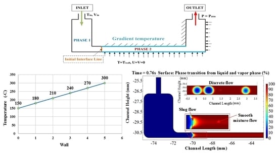
3.4.6. Flow Boiling Phenomenon in the Rectangular Mini-Channel with Increasing Temperature along the Top and Bottom Walls and Flow Patterns.

The gradient temperature is an important parameter that plays a key role during heat transfer applications. The gradient temperature is applied at the top and bottom walls of the rectangular mini-channel. It affects the flow patterns in a manner of increasing progressively. It has a significant impact on the visualization of the boiling flow patterns in the rectangular mini-channel at a different operating time, as indicated in Figure 13. We notice that the phase transition takes place in a relatively short time compared to the time observed in Figure 11 (0.83 s). Figure 13 describes the phenomenon observed in the rectangular mini-channel.

In this study, the flow patterns were captured in three parts of the channel (inlet, middle and outlet areas) to observe what phenomenon happened in the rectangular mini-channel.

At t = 0.76 s, when the temperature reaches the saturation point around 373.15 K, the flow pattern found in Figure 13 [X] nearly the initial interface is slug flow. At a certain distance along the horizontal channel, the transition is happening at high temperatures. There is an appearance of the droplet’s formation in the middle of the channel, as seen in Figure 13 [X_A-X_B]. The size of the droplets is significant because their diameters are close to the small diameter of the channel. The observed flow pattern is the smooth discrete flow. The liquid and the gas are mixed in that area proportionally. The interfacial regions in the vicinity of the round or elliptical droplets have gradation transition zones. It is in line with the flow patterns that were found during the flow boiling of R-134a and R-22 fluids with a circular channel of 0.5 mm [57].

At t = 1.07 s, when much heat transferred from the walls, the observed flow pattern closer to the initial interface, as shown in Figure 13 [Y], is slug flow, which has a smaller geometrical feature due to the density of the fluid flow that decreases with the time. During the phase transition, it is observed some droplets with considerable size and droplets with small sizes at one part in the middle along the horizontal channel, as seen in Figure 13 [Y_A-Y_B]. The flow pattern is classified as a discrete flow. The formed gas and remaining droplets in the channel possess significant proportions. Besides, flow boiling of water in a rectangular metallic microchannel was investigated for a hydraulic diameter of 0.56 mm and a length of 62 mm and it was found that the important flow regimes observed were bubbly, slug, churn, discrete flow and annular flow [26,55]. Compared with this investigation, the obtained results in this study are significant and comparable to the founded flow regimes in experiments above, such as the transition discrete flow and smooth mixture flow.

At t = 2.1 s, the maximum heat flux dissipated is approximately 5.34 MW/m²_, as seen in Figure 14.

The maximum heat flux dissipated at increasing temperature along the top and bottom walls. Due to the applied gradient temperature at the top and bottoms walls of the rectangular mini-channel, the heat flux with increasing temperature is 80.89% higher than the heat flux at constant wall temperature.

At a different coordinate point in the channel that varies with the time, the high heat flux for the point (−69.5, −30.625) is estimated at ~2 × 10⁵ W/m² when the temperature is approximately 315 K as presented in Figure 15 by the green line. At that point, the temperature varies from 293.17 K to 450 K along with the horizontal position in the channel.

The single-phase flow was also investigated with the increasing temperature applied at the top and bottom walls and it is found that there are no boiling effects (Section 2.4, Figure S7, Table S7 in supplementary).

All the obtained heat fluxes in this study are significant for heat transfer and these values lay a foundation for the rectangular mini-channel to be used in different application areas referred to in Table 3. Therefore, it is noticed that the system with increasing temperature presents the highest dissipated heat flux and could practically be implemented in the applications.

4. Conclusions

The numerical study of flow and heat transfer coupled in this rectangular mini-channel with numerous hydraulic diameters allowed us to have a more in-depth knowledge of physical phenomena that govern the flows. The fundamental variable results, including velocity profiles, pressure drops, friction factors were computed. This study using COMSOL presents valuable data obtained through the variation of model parameters. We have demonstrated how to determine the applicability of the rectangular mini-channel in certain industrial areas. The dissipated heat flux for each application area has been estimated from the simulation results. The Reynolds number at the cooling time, convective heat transfer coefficient and fin efficiency of the system are significant to prove the efficiency of the elementary system based on the parameters that have been imposed. According to Newton’s Law of Cooling, the value of the coefficient of convective heat exchange proves that the observed mode is flow boiling in water. Flow boiling heat transfer is efficient inside the mini-channel when the number of Reynolds is less than 400. Therefore, the rectangular mini-channel promotes an excellent heat exchange. Finally, the obtained results from the flow boiling heat transfer in two-phase flow showed that the important flow regimes, including smooth mixture flow and transition discrete flow, have emerged. We have also applied a different temperature gradient at the top and bottom walls of the channels. It is found that the system with the increasing temperature monotonously presents the highest heat flux dissipated compared to other systems without changing the parameters and the geometry of the mini-channel in two-phase flow. That possibly indicates that the flexible channel going through along a tailored route which undergoes a temperature gradient will get a better heat dissipation effect.

References

1. Whitesides, G.M. The origins and the future of microfluidics. Nature 2006, 442, 368. [Google Scholar] [CrossRef]
2. Giri, B. Laboratory Methods in Microfluidics; Elsevier: Amsterdam, The Netherlands, 2017. [Google Scholar]
3. Fabbri, M.; Dhir, V.K. Optimized heat transfer for high power electronic cooling using arrays of microjets. J. Heat Transf. 2005, 127, 760–769. [Google Scholar] [CrossRef]
4. Hamami, A. Simulation de l’écoulement Dans un Minicanal. Ph.D. Thesis, Université de Batna 2, Fesdis, Algeria, 2005. [Google Scholar]
5. King, M.R. Biomedical applications of microchannel flows. In Heat Transf. Fluid Flow Minichannels Microchannels; Elsevier: New York, NY, USA, 2005; pp. 409–442. [Google Scholar]
6. Brand, O.; Fedder, G.K.; Hierold, C.; Korvink, J.G.; Tabata, O. Micro Process Engineering: Fundamentals, Devices, Fabrication and Applications; John Wiley & Sons: Hoboken, NJ, USA, 2013. [Google Scholar]
7. Schmidt, R. Challenges in electronic cooling—Opportunities for enhanced thermal management techniques—Microprocessor liquid cooled minichannel heat sink. Heat Transf. Eng. 2004, 25, 3–12. [Google Scholar] [CrossRef]
8. Ohadi, M.; Choo, K.; Dessiatoun, S.; Cetegen, E. Next Generation Microchannel Heat Exchangers; Springer: New York, NY, USA, 2013. [Google Scholar]
9. Kandlikar, S.G.; Bapat, A.V. Evaluation of jet impingement, spray and microchannel chip cooling options for high heat flux removal. Heat Transf. Eng. 2007, 28, 911–923. [Google Scholar] [CrossRef]
10. Jahan, S.A.; El-Mounayri, H. A thermomechanical analysis of conformal cooling channels in 3D printed plastic injection molds. Appl. Sci. 2018, 8, 2567. [Google Scholar] [CrossRef] [Green Version]
11. Torres-Alba, A.; Mercado-Colmenero, J.M.; Diaz-Perete, D.; Martin-Doñate, C. A New Conformal Cooling Design Procedure for Injection Molding Based on Temperature Clusters and Multidimensional Discrete Models. Polymers 2020, 12, 154. [Google Scholar] [CrossRef] [Green Version]
12. Tuckerman, D.B.; Pease, R.F.W. High-performance heat sinking for VLSI. IEEE Electron Device Lett. 1981, 2, 126–129. [Google Scholar] [CrossRef]
13. Peiyi, W.; Little, W.A. Measurement of friction factors for the flow of gases in very fine channels used for microminiature Joule-Thomson refrigerators. Cryogenics 1983, 23, 273–277. [Google Scholar] [CrossRef]
14. Papautsky, I.; Brazzle, J.; Ameel, T.; Frazier, A.B. Laminar fluid behavior in microchannels using micropolar fluid theory. Sens. Actuators A Phys. 1999, 73, 101–108. [Google Scholar] [CrossRef]
15. Pfund, D.; Rector, D.; Shekarriz, A.; Popescu, A.; Welty, J. Pressure drop measurements in a microchannel. AIChE J. 2000, 46, 1496–1507. [Google Scholar] [CrossRef]
16. Wilding, P.; Pfahler, J.; Bau, H.H.; Zemel, J.N.; Kricka, L.J. Manipulation and flow of biological fluids in straight channels micromachined in silicon. Clin. Chem. 1994, 40, 43–47. [Google Scholar] [CrossRef]
17. Yang, C.Y.; Webb, R.L. Friction pressure drop of R-12 in small hydraulic diameter extruded aluminum tubes with and without micro-fins. Int. J. Heat Mass Transf. 1996, 39, 801–809. [Google Scholar] [CrossRef]
18. Kandlikar, S.G. Fundamental issues related to flow boiling in minichannels and microchannels. Exp. Therm. Fluid Sci. 2002, 26, 389–407. [Google Scholar] [CrossRef]
19. Debray, F.; Franc, J.P.; Maitre, T.; Reynaud, S. Measurement of Forced Convection Heat Transfer Coefficients in Mini-Channels; Mesure des Coefficients de Transfert Thermique par Convection Forcee en Mini-Canaux. Mec. Ind. 2001, 2, 443–454. [Google Scholar]
20. Peng, X.F.; Peterson, G.P. Convective heat transfer and flow friction for water flow in microchannel structures. Int. J. Heat Mass Transf. 1996, 39, 2599–2608. [Google Scholar] [CrossRef]
21. Peng, X.F.; Peterson, G.P.; Wang, B.X. Frictional flow characteristics of water flowing through rectangular microchannels. Exp. Heat Transf. Int. J. 1994, 7, 249–264. [Google Scholar] [CrossRef]
22. Li, J.; Peterson, G.P. Boiling nucleation and two-phase flow patterns in forced liquid flow in microchannels. Int. J. Heat Mass Transf. 2005, 48, 4797–4810. [Google Scholar] [CrossRef]
23. Jing, D.; Song, J.; Sui, Y. Hydraulic and thermal performances of laminar flow in fractal treelike branching microchannel network with wall velocity slip. Fractals 2020, 28, 2050022. [Google Scholar] [CrossRef]
24. Jing, D.; Yi, S. Electroosmotic flow in tree-like branching microchannel network. Fractals 2019, 27, 1950095. [Google Scholar] [CrossRef]
25. Chafaa, N.; Benramdane, H. Simulation Numérique de la Convection Forcée Dans un Canal Horizontal Muni des Sources de Chaleur (Application: Refroidissements des Composants Électroniques). Master’s Thesis, Université de Tlemcen, Chetouane, Algeria, 2015. [Google Scholar]
26. Özdemir, M.R.; Mahmoud, M.M.; Karayiannis, T.G. Flow Boiling of Water in a Rectangular Metallic Microchannel. Heat Transf. Eng. 2020, 1–25. [Google Scholar] [CrossRef] [Green Version]
27. Kandlikar, S.G.; Balasubramanian, P. An Experimental Study on the Effect of Gravitational Orientation on Flow Boiling of Water in 1054 × 197 μm Parallel Minichannels. J. Heat Transf. 2005, 127, 820–829. [Google Scholar] [CrossRef] [Green Version]
28. Kandlikar, S.G. Heat Transfer Mechanisms During Flow Boiling in Microchannels. J. Heat Transf. 2004, 126, 8–16. [Google Scholar] [CrossRef]
29. Lee, P.-S.; Garimella, S.V. Saturated flow boiling heat transfer and pressure drop in silicon microchannel arrays. Int. J. Heat Mass Transf. 2008, 51, 789–806. [Google Scholar] [CrossRef] [Green Version]
30. Squires, T.M.; Quake, S.R. Microfluidics: Fluid physics at the nanoliter scale. Rev. Mod. Phys. 2005, 77, 977. [Google Scholar] [CrossRef] [Green Version]
31. Wen, J.; Gu, X.; Liu, Y.; Wang, S.; Li, Y. Effect of surface tension, gravity and turbulence on condensation patterns of R1234ze(E) in horizontal mini/macro-channels. Int. J. Heat Mass Transf. 2018, 125, 153–170. [Google Scholar] [CrossRef]
32. Cahn, J.W.; Hilliard, J.E. Free Energy of a Nonuniform System. I. Interfacial Free Energy. J. Chem. Phys. 1958, 28, 258–267. [Google Scholar] [CrossRef]
33. Belhadje, A.; Rachid, S.; Bouchnafa, R. Etude Thermo-Énergétique de la Convection Forcée dans les Microcanaux avec un Changement Périodique de la Section Transversale. In Proceedings of the Abou Bekr Belkaid University of Tlemcen Faculty of Technology 3rd Seminar on Advanced Mechanical Technologies, University Abu Bekr Belkaid, Chetouane, Algeria, 8–9 November 2014. [Google Scholar]
34. Hu, J.; Xiong, X.; Xiao, H.; Wan, K. Effects of Contact Angle on the Dynamics of Water Droplet Impingement. In Proceedings of the COMSOL Conference, Boston, MA, USA, 8 October 2015. [Google Scholar]
35. Cengel, Y.A.; Cimbala, J.M.; Turner, R.H.; Kanoglu, M. Fundamentals of Thermal-Fluid Sciences; McGraw-Hill Higher Education Boston: New York, NY, USA, 2012; Volume 3. [Google Scholar]
36. Shah, R.K.; London, A.L. Laminar Flow Forced Convection in Ducts: A Source Book for Compact Heat Exchanger Analytical Data; Academic Press: New York, NY, USA, 1978; Suppl. 1. [Google Scholar]
37. Chen, N.H. An Explicit Equation for Friction Factor in Pipe. Ind. Eng. Chem. Fund. 1979, 18, 296–297. [Google Scholar] [CrossRef]
38. Chen, X.; Hu, Z.; Zhang, L.; Yao, Z.; Chen, X.; Zheng, Y.; Liu, Y.; Wang, Q.; Liu, Y.; Cui, X. Numerical and Experimental Study on a Microfluidic Concentration Gradient Generator for Arbitrary Approximate Linear and Quadratic Concentration Curve Output. Int. J. Chem. React. Eng. 2018, 16. [Google Scholar] [CrossRef]
39. Hassinet, L. Etude De L’ecoulement Laminaire Dans Un Minicanal Par La Methode Des Volumes Finis. Ph.D. Thesis, Université de Batna 2, Fesdis, Algeria, 2008. [Google Scholar]
40. Sahar, A.M.; Wissink, J.; Mahmoud, M.M.; Karayiannis, T.G.; Ashrul Ishak, M.S. Effect of hydraulic diameter and aspect ratio on single phase flow and heat transfer in a rectangular microchannel. Appl. Therm. Eng. 2017, 115, 793–814. [Google Scholar] [CrossRef]
41. Harley, J.C.; Huang, Y.; Bau, H.H.; Zemel, J.N. Gas flow in micro-channels. J. Fluid Mech. 1995, 284, 257–274. [Google Scholar] [CrossRef]
42. Sarkar, D. Thermal Power Plant: Design and Operation; Elsevier: Amsterdam, The Netherlands, 2015. [Google Scholar]
43. At what Temperature Do Conventional Electronics Packages Fail? Available online: https://www.twi-global.com/technical-knowledge/faqs/faq-at-what-temperature-do-conventional-electronics-packages-fail.aspx (accessed on 1 September 2020).
44. Karayiannis, T.G.; Mahmoud, M.M. Flow boiling in microchannels: Fundamentals and applications. Appl. Therm. Eng. 2017, 115, 1372–1397. [Google Scholar] [CrossRef]
45. Oyinlola, M.A.; Shire, G.S.F. Heat Transfer in Low Reynolds Number Flows Through Miniaturized Channels. In Proceedings of the 12th International Conference on Heat Transfer, Fluid Mechanics and Thermodynamics; De Montfort University (DMU): Leicester, UK, 2016. [Google Scholar]
46. Turek, L.J.; Rini, D.P.; Saarloos, B.A.; Chow, L.C. Evaporative spray cooling of power electronics using high temperature coolant. In Proceedings of the 2008 11th Intersociety Conference on Thermal and Thermomechanical Phenomena in Electronic Systems, Orlando, FL, USA, 28–31 May 2008; IEEE: Orlando, FL, USA, 2008; pp. 346–351. [Google Scholar]
47. Bostanci, H.; Van Ee, D.; Saarloos, B.A.; Rini, D.P.; Chow, L.C. Thermal Management of Power Inverter Modules at High Fluxes via Two-Phase Spray Cooling. IEEE Trans. Compon. Packag. Manufact. Technol. 2012, 2, 1480–1485. [Google Scholar] [CrossRef]
48. Kreith, F.; Black, W.Z. Basic Heat Transfer; Harper & Row: New York, NY, USA, 1980. [Google Scholar]
49. Incropera, F.P.; Lavine, A.S.; Bergman, T.L.; DeWitt, D.P. Fundamentals of Heat and Mass Transfer; Wiley: Hoboken, NJ, USA, 2007. [Google Scholar]
50. Advanced Piping Design (Process Piping Design Handbook) (v. II)—PDF Free Download. Available online: https://epdf.pub/advanced-piping-design-process-piping-design-handbook-v-ii.html (accessed on 6 May 2020).
51. Buongiorno, J. Notes on two-phase flow, boiling heat transfer and boiling crises in PWRs and BWRs. In Engineering of Nuclear Systems; MIT Department of Nuclear Science & Engineering (NSE): Cambridge, MA, USA, OpenCourseWare. License: Creative Commons BY-NC-SA; 2010; pp. 1–34. Available online: https://ocw.mit.edu (accessed on 1 September 2020).
52. Guo, Z.Y.; Li, D.Y.; Wang, B.X. A novel concept for convective heat transfer enhancement. Int. J. Heat Mass Transf. 1998, 41, 2221–2225. [Google Scholar] [CrossRef]
53. Kim, S.-M.; Kim, J.; Mudawar, I. Flow condensation in parallel micro-channels–Part 1: Experimental results and assessment of pressure drop correlations. Int. J. Heat Mass Transf. 2012, 55, 971–983. [Google Scholar] [CrossRef]
54. Wu, H.Y.; Cheng, P. Condensation flow patterns in silicon microchannels. Int. J. Heat Mass Transf. 2005, 48, 2186–2197. [Google Scholar] [CrossRef]
55. Cheng, P.; Quan, X.; Gong, S.; Liu, X.; Yang, L. Recent analytical and numerical studies on phase-change heat transfer. In Advances in Heat Transfer; Elsevier: Amsterdam, The Netherlands, 2014; Volume 46, pp. 187–248. [Google Scholar]
56. Tullius, J.F.; Vajtai, R.; Bayazitoglu, Y. A Review of Cooling in Microchannels. Heat Transf. Eng. 2011, 32, 527–541. [Google Scholar] [CrossRef]
57. Zhuan, R.; Wang, W. Flow pattern of boiling in micro-channel by numerical simulation. Int. J. Heat Mass Transf. 2011, S0017931011006661. [Google Scholar] [CrossRef]
Figure 1. Simplified geometry of rectangular mini-channel.
Fluids 05 00151 g001
Figure 2. Schematic representation of boundary conditions.
Fluids 05 00151 g002
Figure 3. Domain mesh: (A) Extremely fine: 130,311 domain elements and 8233 boundary elements, (B) Extra fine: 41,757 domain elements and 4261 boundary elements, (C) Finer: 13,036 domain elements and 2025 boundary elements.
Fluids 05 00151 g003
Figure 4. Velocities profiles of different channels with a different hydraulic diameter at different velocity inlet.
Fluids 05 00151 g004
Figure 5. Drop pressure in Dh = 0.98 mm and Dh = 1 mm along with the horizontal position (mm) of the channel length.
Fluids 05 00151 g005
Figure 6. Friction factor for Dh = 0.5 mm.
Fluids 05 00151 g006
Figure 7. Heat transfer of fluids in the approximate model of two-phase flow from t = 0.45 s to t = 1.1 s with the uniform temperature at the walls: [L-M] Channel inlet, [L1-M1] Channel outlet, contour (values are plotted randomly).
Fluids 05 00151 g007
Figure 8. Heat flux with constant temperature on channel walls at different points varying with the time.
Fluids 05 00151 g008
Figure 9. Variation of the temperature along the walls in blue that have been divided into equal segments. (A) new boundary conditions, (B) increasing temperature, (C) increasing and decreasing temperature.
Fluids 05 00151 g009
Figure 10. The fundamental variables of two-phase flow in the channel in phase field with the increasing and decreasing temperature boundary. Velocity and pressure: (D) channel inlet, (E) channel outlet and temperature contours: (F) random section along the horizontal channel.
Fluids 05 00151 g010
Figure 11. The phase change in the heat transfer model at constant walls temperature: [Q-R] Channel inlet area, [Q1-R1] Channel outlet area.
Fluids 05 00151 g011
Figure 12. Heat flux distribution with constant temperature on channel walls.
Fluids 05 00151 g012
Figure 13. Flow boiling heat transfer with increasing temperature at the top and bottom walls: [X-Y] Channel inlet area, [X1-Y1] Channel outlet area, [XA-XB-YA-YB] Random section of the middle along the horizontal channel.
Fluids 05 00151 g013
Figure 14. Dissipated heat flux distribution with the increasing temperature along the top and bottom walls.
Fluids 05 00151 g014
Figure 15. Heat flux with increasing temperature on channel walls at different points varying with the time.
Fluids 05 00151 g015