Review

Current Trends in Fluid Research in the Era of Artificial Intelligence: A Review

by
Filippos Sofos
1,2,*,
Christos Stavrogiannis
1,
Kalliopi K. Exarchou-Kouveli
2,
Daniel Akabua
2,
George Charilas
2 and
Theodoros E. Karakasidis
1,2
1
Condensed Matter Physics Laboratory, Department of Physics, University of Thessaly, 35100 Lamia, Greece
2
Post-Graduate Program “Applied Physics”, Department of Physics, University of Thessaly, 35100 Lamia, Greece
*
Author to whom correspondence should be addressed.
Fluids 2022, 7(3), 116; https://doi.org/10.3390/fluids7030116
Submission received: 28 February 2022 / Revised: 14 March 2022 / Accepted: 17 March 2022 / Published: 18 March 2022
(This article belongs to the Section Mathematical and Computational Fluid Mechanics)

Abstract

:
Computational methods in fluid research have been progressing during the past few years, driven by the incorporation of massive amounts of data, either in textual or graphical form, generated from multi-scale simulations, laboratory experiments, and real data from the field. Artificial Intelligence (AI) and its adjacent field, Machine Learning (ML), are about to reach standardization in most fields of computational science and engineering, as they provide multiple ways for extracting information from data that turn into knowledge, with the aid of portable software implementations that are easy to adopt. There is ample information on the historical and mathematical background of all aspects of AI/ML in the literature. Thus, this review article focuses mainly on their impact on fluid research at present, highlighting advances and opportunities, recognizing techniques and methods having been proposed, tabulating, and testing some of the most popular algorithms that have shown significant accuracy and performance on fluid applications. We also investigate algorithmic accuracy on several fluid datasets that correspond to simulation results for the transport properties of fluids and suggest that non-linear, decision tree-based methods have shown remarkable performance on reproducing fluid properties.

1. Introduction

Research in fluids spans over a wide range of sizes, from quantum to continuum, and time scales, from picoseconds to hours or more. Traditionally, there have been distinct groups to investigate phenomena at each scale. Multiscale simulation approaches, fueled by high-performance computing architectures, are now a fact, bridging distinct research fields in common platforms. Physics-based descriptions are essential in understanding fluid behavior, as, most of the times, the electronic and atomic properties of the substance affect its overall behavior. Advances in material science have also made possible the conduction of laboratory experiments close to the atomic scale with increased accuracy, while industrial and large-scale research is constantly providing real-case data to guide the research.

1.1. Data Science

Computational science has gone through various stages, from empirical methods to the model-based theoretical paradigm, and the computational third paradigm. Our ability to collect data from various procedures has gone beyond our understanding of it. At present, new techniques and approaches have arisen through the data-driven fourth paradigm, capable of overcoming the limitations of its traditional predecessors [1], based on developing accurate predictions and discovery-based data mining tools on huge datasets. Mathematical modeling, experiments, and computer simulations are three traditional scientific development models that are supported by the fourth paradigm and the evolution of computer science, high-performance computing, ML, and data mining methods [2].
Data used nowadays for physical sciences may be categorized as: (a) material properties from experiments and simulations (physical, chemical, structural, thermodynamics, dynamics, etc.), (b) chemical reaction data (reaction rate, reaction temperature, etc.), (c) image data (scanning electron microscope images of materials, photos of material surfaces, etc.), and (d) data from the literature [3]. These data are discrete (e.g., texts), continuous (e.g., vectors and tensors), in the form of weighted graphs, or image/video data that represent a phenomenon in graphical form. Derived from different sources, it may be of importance to select and weight experimental and simulated datasets as a prerequisite step in the development of thermodynamic property models [4].

1.2. AI/ML in Fluid Research

AI has entered fluid research and led to an explosion of relevant publications that tried to bind together innovative algorithms with human perception [5]. ML is a branch of AI that entails statistical approaches to analyze and build algorithms trained on data and generate predictions about data. It is generally classified into supervised and unsupervised learning, where supervised learning refers to finding predictions for labeled data, while unsupervised learning is used for unlabeled data. During supervised learning, training data provide the knowledge to map inputs to outputs. In unsupervised learning, possible patterns of input data have to be explored first [6]. Some also categorize Reinforcement Learning (RI) as the third ML branch. In RL, training data are not necessary, the model tries to create its own data on the fly and the model is self-trained to improve its accuracy [7].
These ML methods were applied to address many challenges in fluid research, such as statistical processing of experimental data, turbulence modeling, material properties extraction, control pipelines, to mention a few, overcoming the inherent computational burden and/or expensive experimental setups. From another point of view, ML might be seen as a new approach to address traditional fluid mechanics problems in a different way [8]. ML can make predictions for a fraction of the cost of the initial computation time without sacrificing accuracy [9] and can be more computationally efficient as compared to physics-based numerical simulations [10]. Moreover, it can capture data behavior while eliminating irrelevant features, and explain the predictions to devise explainable techniques [11]. The algorithms inferred follow a decision process and make predictions that are usually validated by the same dataset [12]. Traditional numerical approaches often range between prediction accuracy and computational efficiency. However, due to the high computational cost, simulations are limited to small systems, for a small duration, in order to produce findings, close to those obtained in experiments.
The successful application of ML in fluid research is based on six main components: (i) data quality and quantity, (ii) finding input features that can appropriately describe the process, (iii) implementing a validation scheme for the model, (iv) ensuring explainability for the model [13,14], and, in another direction, (v) replacing conventional simulations and reaching predictions at only a fraction of the initial computational cost, without cutting down the accuracy, and capturing important aspects of the data while discarding inessential details, (vi) continually generating high-quality training data [15] by using ML in conjunction with the experiment [16]. The use of the two together complimentarily is what can progress the material discovery.
However, big data availability does not always mean that data are ready to process and analyze. It is a fact that ML is faced with sparse data, due to the high-dimensional space, geometrical implications, boundary conditions, and nonlinear aspects of fluid mechanics. The term “Intelligent Fluid Mechanics” (IFM) has emerged [17], along with the concept of physics-informed neural networks (PINNs), where the underlying flow physics has entered the ML process to strengthen that traditional black-box model consideration [18]. Current trends also include advances in symbolic regression techniques, where symbolic expressions are extracted from data without prior knowledge of the inferred system and, along with statistical learning, dive deep into the physical meaning of data. Physics-based data descriptions are now a fact [19].

1.3. Reviews and Perspectives on Fluid Research and ML

A number of new reviews and perspectives regarding ML and fluids have been published lately. A historical review, spotting past and current developments, along with predicting the future in fluid mechanics, is made by Brunton et al. [20]. ML algorithms are grouped into the three main categories (i.e., supervised, unsupervised, semi-supervised), and characteristics are given, while, emphasis is placed on statistical optimization techniques, Bayesian inference, and the Gaussian Processes. Brenner et al. [8] highlight the need for incorporating quantitative and qualitative training data in various ML applications. It is also stated that ML should be used in conjunction with human intuition and physical reasoning to address the principles of fluid mechanics.
Physics-based decisions are the driving force for trustworthy ML. To embed physical knowledge on the models, researchers are advised to carefully choose model/problem and available data, decide on the proper architecture, design loss functions to quantify performance and guide the learning process, and, finally, implement an optimization method to minimize the loss function over the training data [21]. For applications on fluid thermophysical properties, where data are usually sparse and subject to uncertainties, physical knowledge is also the key to dealing with this. Moreover, ML can serve as a data analysis tool and help to create physical insights and improved understanding to overcome the “black-box” nature of ML models [22].
Technical directions on characterizing fluid flow in pipes are given in the review of Arief et. al, referring to multiphase flows controlled by sensor data [23]. Classical computational methods, such as the speed of sound estimation and Joule–Thomson coefficient, are used in conjunction with ML algorithms (Convolutional Neural Networks, Support Vector Machines, Ensemble Kalman Filter). Turbulence modeling is also a popular research field in current ML applications, where the primary focus has been the exploration of new routes to parametrize unresolved scales in complex flow configurations at high Reynolds numbers. Pandey et al. [24] argue about the connection of big-data analysis, as driven by the research in astronomy and astrophysics, with data analysis in turbulence, suggesting that fluid research can benefit significantly from similar AI applications. Industrial applications can also benefit from large datasets, more advanced ML algorithm techniques, and higher computational power. To obtain data from the field, better sensors with higher data acquisition rates and higher resolution would be an asset, along with new data compression techniques to handle huge datasets [10].

1.4. Aim and Objectives

Taking in mind all directions and perspectives presented in the current literature, in this review, we wish to complement the discussion on ways to explore and benefit from AI and ML in the multifactorial field of fluid research. At first, we cover issues concerning trends and methods used in fluid flows to bridge among scales and provide new insight into multiscale modeling with embedded ML calculations. As a vast number of simulations, experimental, and data from the field are gathered in various databases, we describe the process of fluid properties extraction from the microscopic to the macroscopic level with ML. We also emphasize the concept of extracting physics-based descriptions to solve PDEs and cover all the latest fluid research on turbulence modeling and other CFD fields. Finally, we performed an algorithmic investigation for a number of well-established ML algorithms that were incorporated in fluid research and concluded their performance by investigating a simulation dataset related to the transport properties of fluids. Results have shown that decision-based algorithms perform better on fluid datasets with non-linear behavior. Then, finally, we highlight the fact that, by keeping pace with physical knowledge gathered through extensive research on fluids throughout the years, AI and ML can be means of enriching our computational “reservoir” to tackle existing and unresolved problems.

2. Bridging across Scales

The behavior of an atom in a molecule, liquid, or solid is governed by the force it experiences. If the dependence of this force on the atomic chemical environment can be learned accurately by exploiting big-data techniques, then this capability can be harnessed to speed up simulations [25]. Starting from the “bottom”, ML was used to extract classical potential energy surfaces (PES) from quantum mechanical (QM) calculations, in order to efficiently perform Molecular Dynamics (MD) simulations that take into account quantum effects [26]. Moreover, ML can be used to generate samples from the equilibrium distribution of a molecular system without performing MD altogether, as proposed in the recently introduced Boltzmann Generators, a method based on training on the energy function of a many-body system able to provide unbiased, one-shot samples from its equilibrium state [27].
MD simulations following the Born–Oppenheimer (BO) approximation have become the atomistic modeling standard nowadays and fluids are no exception [28,29]. The main steps include the construction of the PES as a function of the positions of the nuclei so that the calculation of most thermodynamic properties becomes possible [30]. On the other hand, Quantum Mechanics (QM) approaches have the benefit of being derived from fundamental physics and are thus accurate for a wide variety of systems, and the incorporation of the density functional theory (DFT) decreases their computational demand. However, their applicability refers only to smaller time and length scales.
This is where ML has found a receptive field to beat computational barriers. For example, Bayesian techniques, with the aid of experimental measurements, can formulate Schrodinger’s equation for efficient quantum dynamics calculations [31]. Moreover, current research efforts have developed alternative approaches to calculating the PES known as interatomic potential models or force fields (FFs) [32]. The potential energy of a system is seen as the sum of bonded (e.g., bond stretching, angle bending, dihedral torsion) and nonbonded (e.g., van der Waals) atomic interactions to construct an FF model, with partial contributions being calculated from positions, charges, and relative orientations. The Gaussian Approximation Potential (GAP) model was successfully applied to build the potential for liquid methane (CH4), which is a difficult task when approached from first principles because its behavior is dominated by weak dispersion interactions with a significant many-body component [33].
Multiscale modeling can integrate ML to create surrogate models to bridge between the scales [34], as can be seen in Figure 1. Till now, MD simulations have managed to reach a system size of twenty trillion atom simulations, but, still, this is far from representing a real system [35]. Research has shown that the construction of ML interatomic potentials (MLIPs) trained over ab initio MD (AIMD) trajectories could enable the design of an efficient first-principles multiscale modeling, joining the power of DFT with classical MD and continuum simulation methods. To this end, a complex system would be investigated with first principles precision, at no additional computational cost [36].
By learning the dynamics across scales, one at the deterministic macroscale and the other at the stochastic microscale regime may significantly reduce computational effort and time [37]. Techniques were proposed to reduce the number of simulations at the lower scales with the incorporation of the Dissipative Particle Dynamics (DPD) mesoscale method. Data from one physical quantity are used to predict other unobserved quantities and correlate them with aid of Deep Neural Networks (DNNs) [38]. In another example, a DPD model is bound with the Gaussian Process Regression and Discrete Elements Method to investigate the self-diffusion coefficients of colloids, suspension rheology, and microstructure [39]. Another popular mesoscale particle simulation method, Smoothed-Particle Hydrodynamics (SPH) [40,41] was bound to ML by utilizing experimental data for hydrodynamics modeling, suggesting an integrated framework for studying the rheological properties of complex fluids [42].
In addition to atomistic force fields, it was recently shown that, in the same spirit, effective coarse-grained models can be developed by ML [43] and their data projection can be exploited to parameterize upper-scale models in the form of nonlinear PDEs consistent with a continuum theory [44]. It was also shown that parametrization of the traditional FFs for various materials with ML, based on the use of kernel-based methods that incorporate physical symmetries [45], can be exploited to construct coarse-grained (CG) systems in order to bind accurate but computationally expensive ab initio methods with approximate but computationally cheap CG methods [46]. A DNN is incorporated to learn the relationship between the radial distribution functions (RDFs) of simple liquids at various thermodynamic states (ρ, Τ) with LJ potential parameters [47]. Training data is generated by MD and the knowledge is transferred to coarse-grain simple multiatom molecules, with bonded and nonbonded interactions, into a single LJ particle. Details on LJ parameters are given in Section 6.
However, we should always have in mind that fluid research is conquered by many physical principles that restrict the possible ML predictions to those that have a physical meaning [48].

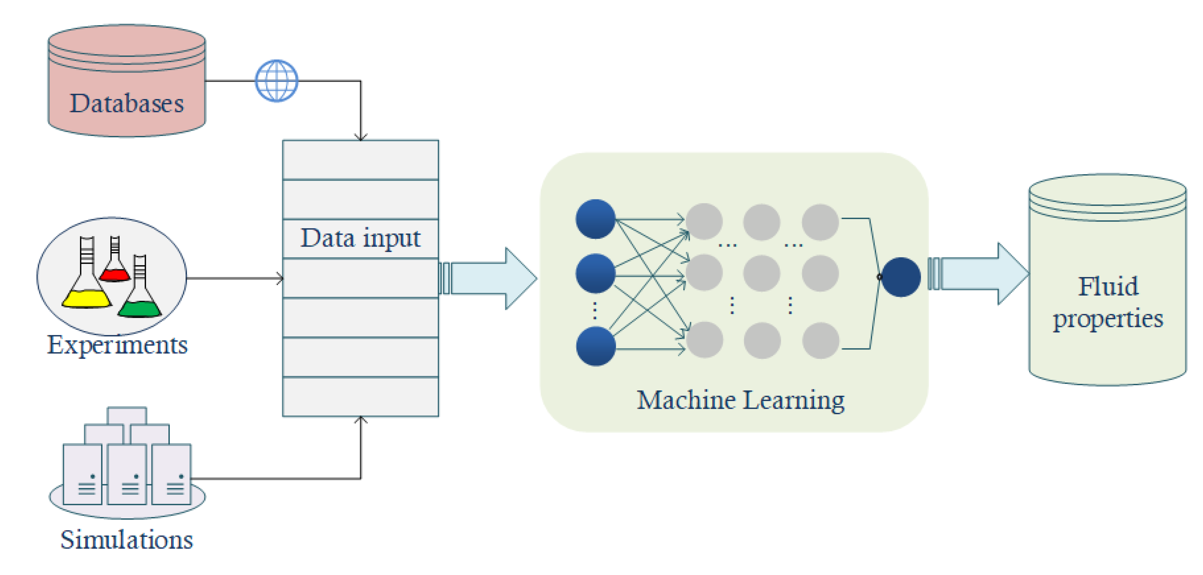
3. Fluid Properties Extraction

Extraction of fluid properties from microscopic calculations has always been a matter of research. Although experimental techniques are the traditional road to acquiring fluid properties, they may be hindered in cases of complex or expensive experimental setups and extreme conditions (e.g., high temperature or pressure). Based on relations from statistical mechanics, empirical relations that have matured over the years, and exploiting MD simulation results, the accuracy of the thermodynamic properties obtained is comparable with those obtained experimentally [49,50].
Data available to the research community has faced a breakdown since the introduction of the Materials Genome Initiative in 2011, aiming to foster material research with data exploitation [51]. In this framework, various electronic databases and journal datasets, containing the calculated properties of existing and hypothetical materials were created and are available online [52,53,54,55]. These efforts have made available a vast number of high-quality computational and experimental physical science data. As a result, a thorough data investigation for structure, patterns, and functional relationships arising from various processes and activities is of critical importance. Finding relationships could lead to novel applications for fluid research, such as, for example, the discovery of water splitting for hydrogen production [56].
The Lennard-Jones (LJ) fluid [57] is usually incorporated in fluid simulations at the atomistic level as the theoretical basis to investigate and calculate physical properties in terms of speed and convenience. For example, the RDF is determined by ML methods. In simple fluids that are dominated by pairwise interactions, structurally based macroscopic observables can be expressed using standard thermodynamic relations containing the RDF. Therefore, once a functional form for the RDF is known, it provides a direct route to generate the thermodynamic properties of the LJ system [15]. The use of different ML models to predict diffusion rates for a well-defined Lennard-Jones (LJ) fluid is also explored [58]. Current studies have shown that symbolic regression techniques, an ML method that is based on genetic programming and proposes analytical expressions to predict the system’s behavior [59], have also given extraordinary results on diffusion coefficient predictions [19].
In water research, density, vaporization enthalpy, self-diffusion coefficient, and viscosity, were obtained from a number of MD simulations that provided the training data to feed a neural network [60]. A general ML framework based on support vector regression (SVR) for predicting the PVT properties of pure fluids and their mixtures is presented in [61]. More properties that can be calculated with ML modeling include solubility prediction in organic solvents and water [62], the prediction of melting points [63], density and viscosity of biofuel compounds [64], FCC diffusion barriers [65], and more.
A general framework for fluid properties extraction is presented in Figure 2.

4. Physics-Based CFD

Computational Fluid Dynamics include numerical techniques that aim to increase the speed of fine-grid simulations, develop turbulence models with different levels of fidelity, and produce reduced-order models (ROMs). Proper Orthogonal Decomposition (POD) and Galerkin Projection techniques are among those used to create ROMs. These methods are sensitive to parameter changes and lack robustness, in a way that they cannot account for transient or multi-scale phenomena [66,67]. ML techniques were used in conjunction with PODs to reduce the system’s dimensionality [68]. Fluid behavior is mainly approached by the Navier-Stokes equations, but solving these equations remains challenging, as it demands increased computational cost to acquire fine spatiotemporal features.
By incorporating ML methods, such as DNNs, the equations can be solved on coarser grids by replacing the components mostly affected by the resolution loss with better performing learned alternatives, such as learned solvers, learned interpolation, and learned correction. This hybrid approach combines physical intuition with data science, and this can be the pathway to generalization [69]. It has become common sense that in high-resolution grids, complex network architectures, such as convolutional neural networks (CNNs) are a powerful tool to handle big data [70].
Physics-Informed Neural Networks (PINNs) are currently becoming a standard in computational science. This concept was introduced to describe a class of universal function approximators, capable of encoding the underlying physical laws behind a given dataset [18], and their current advancement has brought the conservative PINNs (cPINNs) and extended PINNs (XPINNs), which employ domain decomposition in space and in time-space, respectively [71]. Prediction capabilities of DNNs keep pace with the physical conservation laws of momentum, mass, and energy, in metal thermal-fluid flows, trained by FEM simulation data and ensuring minimum loss [72].
Another application is based on the sparse regression technique, where the terms of the governing PDE that most accurately represent the data from a large library of potential candidate functions are calculated. In a Eulerian or a Lagrangian framework, the method proposed in [73] is capable of rediscovering a broad range of physical laws, e.g., Navier–Stokes, from time-series data. Physical laws originating from the Navier–Stokes equations were accurately harnessed, as well, by Hidden Fluid Mechanics (HFM), a physics informed deep learning framework that gives pressure and velocity fields in 2D–3D flows, even in cases where direct measurements may not be possible [74].
Particle fluid simulations can also be accelerated by embedding ML. For example, the derivation of a kinematic equation for finite-size particles that combines ML and physical explanation was proposed [75]. It is based on training the model to learn the mismatch between the implied dataset and an imperfect model containing the physical information. Generalization is achieved as such methods are not restricted by particle size and experimental data can be accurately incorporated and extrapolated in regions where they are not available.
For multiphase flows, hybrid-ML applications were developed and showed a promising solution to model flow behavior. The main objective here is the prediction of flow patterns by using pressure drop data. In a purely data-driven manner, neural network techniques were employed [76], while, in hybrid physics-based and data-driven ML, better accuracy and deeper understanding of the model were achieved [77]. NN techniques were further exploited to create coarse-grained CFD models for Thermal Hydraulics, for the design and safety of Nuclear Power Plants [78]. Purely data-driven techniques were further incorporated for fluid flows in porous media. Artificial neural networks have been the usual choice for training and prediction for a variety of problems in petroleum engineering, in CO2 geological sequestration, and permeability prediction [79,80].
Reynolds Averaged Navier Stokes (RANS) turbulence models are probably the most demanding computational field in CFD. In the last decade, DNNs have become the dominant method to cope with them, and performance gains are now achieved over competing state-of-the-art methods [81]. The incorporation of the XGBoost algorithm has also given accurate predictions in turbulence simulations [82]. An ML-PDE, coarse-grained strategy on a two-dimensional turbulent problem has resulted in corrected solution trajectories that were consistent with the solutions computed at a much higher resolution in space and time [83]. Moreover, new ML-based reconstruction techniques were developed, capable of estimating fluid flow fields from limited measurements, which can be a valuable technique when dealing with small data applications [84].
The new pathway to understanding complex fluid flows goes through visualization. High-resolution images are exploited to extract and calculate system properties through specialized DNN architectures, such as density, velocity, and vorticity. In terms of programming effort, DNNs are able to capture complex features of the system under investigation, as long as GPU or CPU clusters are carefully used in a parallel procedure [85].
It becomes clear that when CFD is combined with ML methods, it is possible to improve simulations without sacrificing accuracy and generalization. On the other hand, it should be pointed out that ML is not a one-for-all solution. It is a fact that complex ML methods, such as DNNs, are hard to implement and do not function with small datasets, as, for example, limited data acquired from an expensive or time-consuming experiment. Thus, it is of importance to spot fields where classical numerical methods are more accurate and efficient [86].

5. Algorithms for Fluid Flows

Next, we present the most common ML algorithms which were successfully incorporated in fluid investigation. We point out that these are not the only algorithmic implementations used in fluid (or, materials, in general) research, nevertheless, we chose an indicative set that has been widely referred to in the literature. More specifically, we employ the regression version of Multiple Linear Regression (MLR), Lasso, Ridge, Support Vector Machines (SVM) in three different instances, the Gaussian Process (GPR), k-Nearest Neighbors (k-NN), Decision Tree (DT), Random Forest (RF), Gradient Boosting (GB), and Multi-Layer Perceptron (MLP). In graphical form, these are shown in Figure 3. We excluded Deep, Convolutional, and Recurrent Neural Network approaches from this study since they demand complex implementations and can be seen as a distinct field of research for huge datasets and/or graphical data analysis. DNNs are expected to have a central role in future molecular representations with chemical information [87].

5.1. Multiple Linear Regression

In a simple regression model, if Y is the predicted variable, X is the input variable, b is the bias term and w is the weight of the variable, then
Y = w X + b
For a set of n independent input variables (e.g., the regressor), the multiple linear regression model (MLR) is
Y = i = 1 n w i X i + b
In the above expression, w 1 , w 2 , , w n are a set of unknown parameters, representing the impact of the respective X 1 ,   , X n independent inputs on the dependent variable Y and b is the bias term which equals the unknown error imposed in the model.

5.2. Ridge Regression

The ridge regression method was introduced in order to overcome poor predictions when linear regression fails to capture data behavior. In cases where data have many or highly correlated variables, then the Ordinary Least Squares (OLS) parameter estimates have low bias but high variance, which leads to high Mean Squared Error (MSE) values [88]. This fact makes the OLS method unreliable. Regularizing methods, such as ridge regression, are accoutering to counter this undesirable case [89].
Ridge regression shrinks the regression coefficients by imposing a penalty on their size. The coefficients minimize a penalized residual sum of
β ^ r i d g e = a r g m i n i = 1 N y i β 0 j = 1 p x i j β i j 2
subject to j = 1 p β j 2 t , where t is related to the amount of shrinkage.
In ML linear regression, a common problem is the fact that it needs a higher number of training samples than the number of features, while ridge regression may function with fewer training samples needed to achieve acceptable results [90,91]. Ridge regression was successfully used for materials science, in predictions of liquid quality and craniofacial reconstruction algorithms, among others [92,93,94].

5.3. Lasso Regression

The least absolute shrinkage and selection operator (Lasso) regression method is another linear-based method that resembles ridge, with subtle but important differences. It imposes a constraint on the model parameters, which “shrinks” the coefficients towards zero. In this way, the sum of the absolute value for OLS coefficients is forced to be less than a fixed value. It tries to select a small predictive feature subset out of a high dimensional and is considered an effective technique for shrinkage and feature selection [95]. The Lasso estimate is given by [96]
β ^ l a s s o = a r g m i n i = 1 N y i β 0 j = 1 p x i j β i j 2  
subject to j = 1 p β j t .
In Figure 3b,c, the ridge and the Lasso regression are depicted for a general case. The residual sum of squares is shrunk by a factor β j for Lasso and β j 2 for ridge. A detailed discussion on the methods can be found in [96].
Lasso was applied, among others, to predict fluid flow in porous media [97], oil flow rate [98], and flow-field reconstruction from sparse data [99].

5.4. Support Vector Machines

Support Vector Machine (SVM) is an effective classification and regression analysis method that could, under certain circumstances, replace artificial neural networks in fluid research [100]. SVM incorporates kernel functions that map the input to a higher dimensional feature space through kernel functions, such as Linear, Polynomial, or Radial Basis Functions. Although computationally demanding, SVM does not depend on the dimensionality of the input space and can be easily generalized. It further provides the opportunity to select the error margin [101]. In fluid research, the SVM approach was recently implemented in the areas of hydrology and river flow forecasting [102].

5.5. Gaussian Process Regression

The Gaussian Process (GP) is a non-linear regression method that predicts the values of an unknown function by using input data as evidence. It may deal with noisy data and can estimate the uncertainties involved in their predictions [103]. Its basis comes from the Bayesian probability theory and is closely connected to other regression techniques.
It was successfully introduced in the construction of the GAP model and has found many applications in many computational demanding problems in materials science. A very interesting review with all related theories and applications can be found in [104].

5.6. k-Nearest Neighbors

The k-Nearest Neighbor (k-NN) algorithm does not need parameters to operate and can be used for classification and regression tasks [105]. The classifier in the (k-NN) algorithm selects k training marks that are close to a test data point x and predicts the approach that relies on these training sets. The Euclidean distance metric is used to compute the distance between test and training data points. After grouping the calculated distances from the lowest to the highest, the most prevalent outcome from the first k rows is the predicted result [106]. The prediction begins when the k-value is chosen, and the regression probability is averaged for the k-Nearest Neighbor. The prediction’s result can then be computed using
g = 1 k i = 1 k g i
where gi is the ith sample size of data and g is the result of query point prediction [107].

5.7. Decision Trees

The Decision Tree (DT) is a supervised ML algorithm that creates a tree-like conceptual framework from training data. It is reminiscent of a flowchart. Each node represents a test on a feature, and each branch represents the result of the test. The DT model’s response is predicted by following the decisions from start to end node [106]. The feature space is partitioned recursively based on the splitting attribute. Each final region is assigned a value to estimate the target output. The tree can be represented as a function [108]
F Θ x = l l e a v e s Τ θ l I l x
The DT algorithm was successfully employed in fluids and material research to detect water pipes that are imminent to fail [109] and to predict thermoelectrically materials scale [6]. It is considered an easy choice to use, but it is often used along with other methods as data may be overfitted [110].

5.8. Random Forest

Random Forest (RF) is a multiple decision tree supervised ML algorithm. The tree classifiers are randomly chosen from the given input features and generate decision trees from the training dataset with replacement using the bootstrap method. The RF algorithm operates in two steps: the forest is generated in the first step, and prediction is performed at the second step using the rule generated in the first step. There is a solid correlation between accuracy and the number of trees in the forest, which means that more accurate outcomes can be achieved by increasing the number of trees in the forest. As it reduces the problem of overfitting, RF is thought to be superior to a single decision tree. The best output of the model is obtained by averaging the outcomes of individual decision trees using
Y = 1 B j = 1 b Y b X
where each decision tree is indicated by Yb and is trained on X′ unknown scenarios.
The symbol B stands for the number of decision trees. This algorithm’s operation begins with the selection of a sample number, after which a decision tree is constructed for each sample. Following that, each decision tree predicts the outcome based on the given input parameters, and voting is used to select the best one from all the predicted results. Eventually, the final prediction result is determined by a majority vote. The bootstrap procedure does not select approximately one-third of the database. This is typically referred to as out-of-bag data. This out-of-bag data is then used by the trees to domestically validate the states, increasing accuracy, and improving RF performance [1,2].
RF algorithms are applied in many scientific studies, and especially in fluids, they have shown remarkable performance, such as the prediction of slip lengths [111] and diffusion coefficients [112].

5.9. Gradient Boosting

Gradient Boosting (GB) is yet another effective method for dealing with nonlinear classification and regression problems. In this method, a group of base learners (simple algorithms) is combined to create a strong learner that can solve a specific problem. Among the most renowned GB tweaks is to use regression trees as base learners, which is known as Tree Gradient Boosting. The primary objective of gradient boosting, provided a training dataset D, is to figure estimation of the function F(x), which maps variables x to their output values y, by diminishing the expected value of a given loss function, F m x = L y , F x . Gradient boosting generates a weighted sum of functions as an additive estimation of F(x) as
F m x = F m 1 x + p m h m x
where p m is the weight of the mth function, h m (x). If the iterative process is not properly regularized, this algorithm may suffer from over-fitting [113]. GB algorithm and its tweaks are summarized as high-quality predictors in heat transfer of oscillating heat pipes [114], as oil flow rate predictors from a simple subsea production system [115], and great performers in the diagnostic classification of cancers [116].

5.10. Artificial Neural Networks

Artificial Neural Networks have taken many forms in the past years and are widely incorporated in the case of big data applications. They are based on the Perceptron, the digital analog to a biological neuron. The Multi-Layer Perceptron comprises internal layers between input and output nodes, increasing the complexity, but, on the other hand, is trained efficiently to achieve better statistics. The number of hidden layers is usually determined by trial and error.
Furthermore, the essence of these models enables them to confront nonlinear prediction problems. This method depends on discovering the ambiguous connection in the process to learn the problem-solving method for achieving the output. For this objective, a massive quantity of data is used in the training step, and the proper output is calculated using the connection discovered through that stage. A neuron K can be expressed by the following two Equations as
y k = f u k + b k
u k = i = 1 N w k i x i
where x1, x2,…, xn are the input data, wk1, wk2,…, wkn are the neuron’s connection weights, uk is the linear output of the linear combination of weighted inputs, bk is the bias term, f is the activation function, and yk is the neuron’s output data (signal).

5.11. Symbolic Regression

The process of understanding physical problems usually goes through a well-defined mathematical equation, which can be interpretable and generalizable to extract meaningful information [117]. A core challenge for both physics and ML is symbolic regression (SR): finding a symbolic expression that matches data from an unknown function [118], by incorporating mathematical operators from infinite space, without prior knowledge of the system’s behavior.
The advantage of SR over other ML models is that it provides analytic expressions which can be readily generalized, and which facilitate the understanding of the underlying physics, with decreasing likelihood of overfitting. This is particularly applicable to the fields of physics and material science, as most of the physical laws, when expressed as equations, are relatively mathematically simple [119]. It also has the potential to replace black-box ML models with simple and accurate symbolic equations.
One of the downsides of SR, however, is that the dimensionality of the input space needs to be relatively small [120]. High data dimensionality makes the model search space far too large for any purely data-driven approach to be tractable [121] and, sometimes, the space of candidate equations is huge increasing the complexity of the proposed expression.

5.12. Performance Metrics

Calculations on error statistics that define the success of an algorithm under investigation method usually refer to R 2 , MSE, and MAE, as shown in Equations (11)–(13).
The R 2 is calculated from the formula:
R 2 = 1 i = 1 N Y e x p . , i Y ¯ exp . 2 i = 1 N Y e x p . , i Y p r e d . , i 2
where Y ¯ e x p . is the mean value of the expected output.
The Mean Squared Error (MSE):
M S E = 1 n i = 1 n Y i Y ¯ 2
where Y i = Y e x p . , i Y p r e d . , i and Y ¯ = 1 n i = 1 n Y i .
The Mean Absolute Error (MAE) is:
M A E = 1 n i = 1 n Y i Y ¯

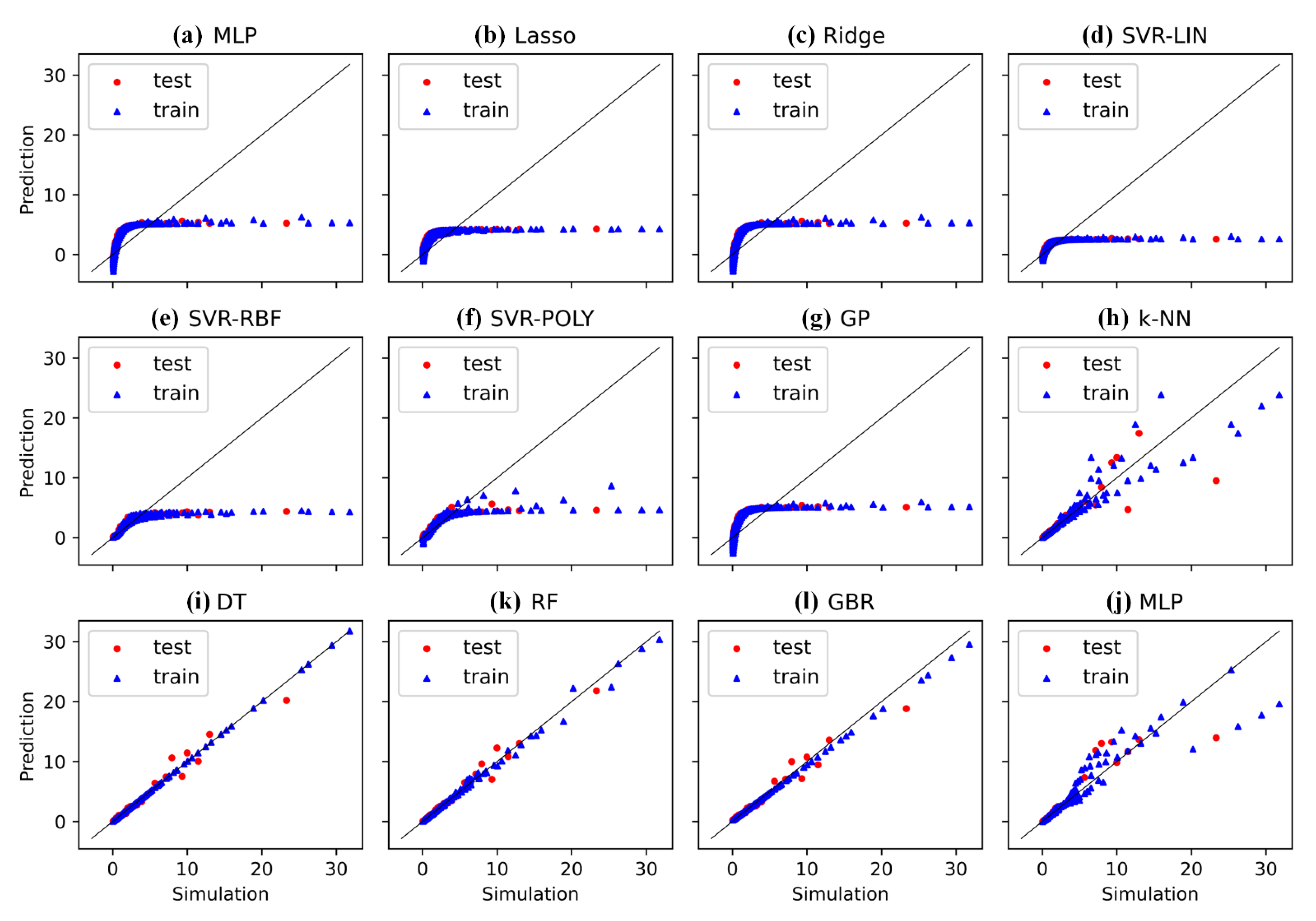
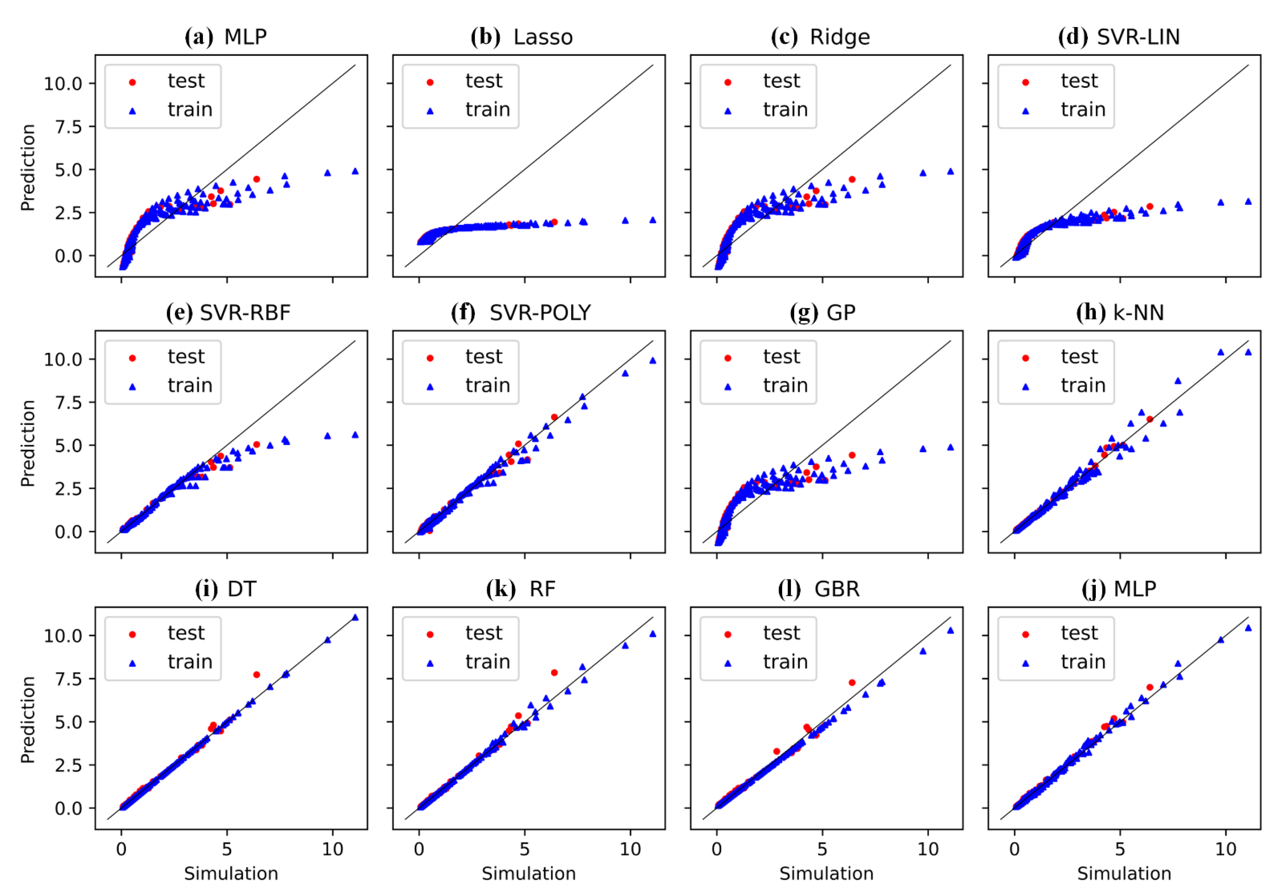
6. Comparative Investigation

In this work, 12 regression algorithms were implemented in order to assess their behavior on fluid simulation datasets and investigate applicable fields in fluid investigation cases. Datasets employed refer to simulation results for LJ fluid transport properties, such as the diffusion coefficient, shear viscosity, and thermal conductivity for bulk and confined systems.
The LJ 12-6 potential is given by
u L J = 4 ε σ r i j 12 σ r i j 6
where the cut-off radius is rc = 2.5σ. Values of the characteristic length and energy, σ and ε, and the masses of the particles are σf = σw = 0.3405 nm (w: wall and f: fluid), ε f / k B = 119.8 K , and m = 39.95 a.u. More details can be found on [122].
The transport properties for the bulk fluids are given for density–temperature (ρ-T) inputs that cover a wide range of fluid phases, from gas to dense fluid [123,124,125]. The confined transport properties refer to Poiseuille-flow model parameters, such as the distance between the plates ( h ), the interaction ratio between wall/fluid particles ( ε w / ε f ) and the external force that drives the flow ( F e x t ), which is the equivalent of the driving pressure used in MD simulations [126]. Datasets can be found from the respective references.
Although being investigated for the theoretical LJ fluid model, these results could be easily extrapolated to real pure fluids [127], providing a macroscale value for the three transport properties, extracted from microscopic calculations.
During preprocessing, the dataset is divided into training points to feed the ML models and testing points to validate predictions (80/20). The normalization stage removes the mean and scales to unit variance according to
x - = x x m e a n x s t d
The two models investigated here are shown in Figure 4. For the Poiseuille flow model, input parameters are the ε w ε f ratio, the distance between the plates, h , and the external force that drives the flow, F e x t . In both systems, the outputs are the diffusion coefficient, the shear viscosity, and the thermal conductivity.
Metrics for diffusion coefficient data, i.e., R2, MSE, and MAE, are shown in Table 1. It is observed that the tree-structured algorithms such as RF and DT have shown optimal performance in all metrics for the bulk diffusion simulation dataset, followed by the GBR model. Moreover, MLP, which is a neural network with backward calculation capability, could also be employed for studying such datasets, as long as the proper implementation concerning the number of nodes and hidden levels is investigated. All other algorithms present low R2 and high residual errors.
Nevertheless, fitting on the confined diffusion data is quite different. Here, there is an indication of linear dependence between the three inputs ( h , ε w / ε f , F e x t ) and the output D c and most linear and/or polynomial-based algorithms (i.e., MLR, Ridge, SVR-LIN, SVR-POLY) show high R2 and small residual errors. The weakest choices are Lasso and DT.
The identity plots of Figure 5 and Figure 6 reveal and verify the findings from Table 1. We observe that the tree-structured algorithms, such as RF and DT, fit well on the bulk diffusion simulation dataset, with GBR, MLP, and k-NN models presenting an acceptable fit behavior. In contrast, linear-based methods, such as MLR, Lasso, Ridge, SVR, and GP, have shown poor fit on diffusion data. For the confined, Poiseuille flow model, we obtain the fitting results of Figure 6a–j. The dataset employed for this case (N = 54) is significantly smaller compared to the bulk diffusion case (N = 319). However, these data are representative of liquid LJ flows, extracted by the same MD method, and were previously pre-processed and verified [126]. It was shown that most algorithmic predictions fit well-to-acceptable on simulation data, except for Lasso, in which data points deviate significantly from the identity line.
In Table 2 we observe that most of our models, with the exception of Lasso, fit well on shear viscosity for the bulk LJ fluid dataset, reaching R2 = 99.7% for the k-NN. We note that, after investigation, it is concluded that the number of nearest neighbors that gives this result is k = 2 (Figure 7). On the contrary, k-NN fails to incorporate shear viscosity behavior in confined systems (Figure 8), and only GB, RF and DT show acceptable fit.
In Table 3, thermal conductivity metrics are presented. As in shear viscosity, most of the models, with the exception of Lasso, fit well on simulation data for the bulk LJ fluid dataset. Choices of good performance, for both bulk and confined data, seem to be RF, DT, GB, and MLP. These findings are also verified by the identity plots in Figure 9 and Figure 10.
The application of 12 widely used algorithms on LJ fluid transport properties data has shown a general motive that may be extrapolated to other datasets as well. In most cases, RF, DT, GB, and MLP methods perform well and can be incorporated in cases where ML predictions could effectively replace timely and hardware demanding simulations or expensive experimental procedures. Linear-based models, such as MLR, Lasso, Ridge, SVR-linear may be used only in some cases.
In terms of performance, our findings have shown fine agreement with the literature results. There are many references that focus only on the performance of ANN and DNN architectures, with various hidden levels, weights, and node functions [128,129,130]. Nevertheless, RF is, most of the time, an algorithmic choice that finds hidden data patterns (see, for example, LJ fluid properties extraction in [111,112]), performs better than SVR and Adaboost DT on RANS simulation results [131] and fluid drilling challenging problems [132]. Gradient-boosting methods have been found to perform better on relatively small datasets compared to ANN, while ANNs are usually the best choice for large datasets concerning dense gas-particle flows [133].
The algorithmic computational cost has not been a subject of investigation of this review. All algorithms showed fast response to input data since datasets are relatively small. We focused on highlighting the increase in computational speed when ML data-driven methods are applied compared to classical simulation methods. The literature results suggest that MLPs and RFs are computationally intensive when the input is multi-parametric, in contrast to SVR, which is faster [70]. However, fast execution is not always preferrable to choose since the additional computational cost may be evidence of robustness, and this is something that was verified by our results.
We conclude that non-linear and, especially, tree decision-based methods can reproduce the initial dataset effectively. However, one has to be very skeptical when suggesting a universal approach that could replace, partially or totally, well-established theoretical, empirical, or other simulation methods that were incorporated for fluid research insofar. Our investigation wishes only to reveal trends and behaviors and open the road towards embedding ML techniques and procedures to classical numerical approaches.

7. Conclusions and Future Perspectives

ML algorithms, although being massively incorporated only in the last few years, have been well-defined and the research community supports their application in most fields of science and engineering. The literature research in this work has revealed that the majority of fluid dynamics and mechanics applications are currently investing in Deep Neural Network applications on classical CFD problems, from finding solutions to PDEs to analyzing high-fidelity fluid-related images. Nevertheless, we showed that there is an alternative way to facilitate ML for fluids. Non-linear, tree-based algorithms, much simpler than DNNs and easy to implement, will continue to attract research interest, providing a fast and accurate framework that can go through every fluid application that infers some amount of data.
We expect that AI and ML methods will become standard computational tools to assist simulations and experimental analysis in the future, without the need to emphasize their use. As available data continues to grow, fluid mechanics have only to benefit from ML and novel AI techniques. Data availability and coupling with experimental, theoretical, empirical, simulation, and novel ML methods offer the potential to significantly boost fluid mechanics to a new direction. Therefore, it is of critical importance to keep all databases open to research. Data science is now part of fluid research and synergistic platforms will keep gaining ground.

Author Contributions

F.S.: Conceptualization, Supervision, Writing, Methodology, Visualization. C.S. and K.K.E.-K.: Writing, Software, Visualization. D.A. and G.C.: Software, Visualization. T.E.K.: Supervision, Review and Editing. All authors have read and agreed to the published version of the manuscript.

Funding

We acknowledge support from the project “A Computational frAmework for MIcroscopic calculations and macroscopic predictions with NOvel machine learning methodS (CAMINOS)”, which is implemented in the context of a grant by the Center of Research Innovation and Excellence of U.Th., funded by the Special Account for Research Grants of U.Th.

Institutional Review Board Statement

Not applicable.

Informed Consent Statement

Not applicable.

Data Availability Statement

All datasets are available in the respective research papers: doi:10.1063/1.1786579, doi:10.1063/1.1421362, doi:10.1016/j.chemphys.2008.06.013, doi:10.3390/fluids6030096 (accessed on 10 January 2022).

Conflicts of Interest

The authors declare no conflict of interest.

Nomenclature

English Symbols
b bias term
Bnumber of decision trees in RF method
Ddiffusion coefficient
F e x t external driving force
F Θ DT function estimation
F m GBR   function   estimation
giith sample size of data for k-NN regression
gthe result of query point prediction for k-NN regression
h channel width
h m (x)function for GBR method
I l DT indicator function
knumber of neighbors for k-NN regression
kBBoltzmann constant
mparticle mass
MAEMean Absolute Error
MSEMean Squared Error
Nnumber of particles
p m weight for GBR method
R 2 coefficient of determination
r i j distance vector between ith and jth atom
Ttemperature
u ( r i j ) LJ potential of atom i with atom j
w weight of the variable
X’number of unknown scenarios in RF method
X input variable
Y predicted variable
Ybdecision tree in RF method
Y ¯ exp . mean expected output
Y ¯ pred . mean predicted output
Greek Symbols
β ^ r i d g e penalized residual sum for Ridge regression
β j shrinkage factor
β ^ l a s s o Lasso regression estimate
εenergy parameter in the LJ potential
θ l DT decision path
λthermal conductivity
μcoefficient of shear viscosity
ρfluid density
σlength parameter in the LJ potential

References

  1. Agrawal, A.; Choudhary, A. Perspective: Materials Informatics and Big Data: Realization of the “Fourth Paradigm” of Science in Materials Science. APL Mater. 2016, 4, 053208. [Google Scholar] [CrossRef] [Green Version]
  2. Agrawal, A.; Deshpande, P.D.; Cecen, A.; Basavarsu, G.P.; Choudhary, A.N.; Kalidindi, S.R. Exploration of Data Science Techniques to Predict Fatigue Strength of Steel from Composition and Processing Parameters. Integr. Mater. Manuf. Innov. 2014, 3, 90–108. [Google Scholar] [CrossRef] [Green Version]
  3. Wei, J.; Chu, X.; Sun, X.; Xu, K.; Deng, H.; Chen, J.; Wei, Z.; Lei, M. Machine Learning in Materials Science. InfoMat 2019, 1, 338–358. [Google Scholar] [CrossRef]
  4. Paulson, N.H.; Zomorodpoosh, S.; Roslyakova, I.; Stan, M. Comparison of Statistically-Based Methods for Automated Weighting of Experimental Data in CALPHAD-Type Assessment. Calphad 2020, 68, 101728. [Google Scholar] [CrossRef]
  5. Frank, M.; Drikakis, D.; Charissis, V. Machine-Learning Methods for Computational Science and Engineering. Computation 2020, 8, 15. [Google Scholar] [CrossRef] [Green Version]
  6. Wang, T.; Zhang, C.; Snoussi, H.; Zhang, G. Machine Learning Approaches for Thermoelectric Materials Research. Adv. Funct. Mater. 2020, 30, 1906041. [Google Scholar] [CrossRef]
  7. Alexiadis, A. Deep Multiphysics: Coupling Discrete Multiphysics with Machine Learning to Attain Self-Learning in-Silico Models Replicating Human Physiology. Artif. Intell. Med. 2019, 98, 27–34. [Google Scholar] [CrossRef]
  8. Brenner, M.P.; Eldredge, J.D.; Freund, J.B. Perspective on Machine Learning for Advancing Fluid Mechanics. Phys. Rev. Fluids 2019, 4, 100501. [Google Scholar] [CrossRef]
  9. Schmid, M.; Altmann, D.; Steinbichler, G. A Simulation-Data-Based Machine Learning Model for Predicting Basic Parameter Settings of the Plasticizing Process in Injection Molding. Polymers 2021, 13, 2652. [Google Scholar] [CrossRef]
  10. Goh, G.D.; Sing, S.L.; Yeong, W.Y. A Review on Machine Learning in 3D Printing: Applications, Potential, and Challenges. Artif. Intell. Rev. 2021, 54, 63–94. [Google Scholar] [CrossRef]
  11. Kailkhura, B.; Gallagher, B.; Kim, S.; Hiszpanski, A.; Han, T.Y.-J. Reliable and Explainable Machine-Learning Methods for Accelerated Material Discovery. Npj Comput. Mater. 2019, 5, 108. [Google Scholar] [CrossRef]
  12. Sofos, F. A Water/Ion Separation Device: Theoretical and Numerical Investigation. Appl. Sci. 2021, 11, 8548. [Google Scholar] [CrossRef]
  13. Roscher, R.; Bohn, B.; Duarte, M.F.; Garcke, J. Explainable Machine Learning for Scientific Insights and Discoveries. IEEE Access 2020, 8, 42200–42216. [Google Scholar] [CrossRef]
  14. Vasudevan, R.K.; Choudhary, K.; Mehta, A.; Smith, R.; Kusne, G.; Tavazza, F.; Vlcek, L.; Ziatdinov, M.; Kalinin, S.V.; Hattrick-Simpers, J. Materials Science in the Artificial Intelligence Age: High-Throughput Library Generation, Machine Learning, and a Pathway from Correlations to the Underpinning Physics. MRS Commun. 2019, 9, 821–838. [Google Scholar] [CrossRef] [Green Version]
  15. Craven, G.T.; Lubbers, N.; Barros, K.; Tretiak, S. Machine Learning Approaches for Structural and Thermodynamic Properties of a Lennard-Jones Fluid. J. Chem. Phys. 2020, 153, 104502. [Google Scholar] [CrossRef]
  16. Sun, W.; Zheng, Y.; Yang, K.; Zhang, Q.; Shah, A.A.; Wu, Z.; Sun, Y.; Feng, L.; Chen, D.; Xiao, Z.; et al. Machine Learning-Assisted Molecular Design and Efficiency Prediction for High-Performance Organic Photovoltaic Materials. Sci. Adv. 2019, 5, eaay4275. [Google Scholar] [CrossRef] [Green Version]
  17. Zhang, W.-W.; Noack, B.R. Artificial Intelligence in Fluid Mechanics. Acta Mech. Sin. 2022, 1–3. [Google Scholar] [CrossRef]
  18. Raissi, M.; Perdikaris, P.; Karniadakis, G.E. Physics-Informed Neural Networks: A Deep Learning Framework for Solving Forward and Inverse Problems Involving Nonlinear Partial Differential Equations. J. Comput. Phys. 2019, 378, 686–707. [Google Scholar] [CrossRef]
  19. Papastamatiou, K.; Sofos, F.; Karakasidis, T.E. Machine Learning Symbolic Equations for Diffusion with Physics-Based Descriptions. AIP Adv. 2022, 12, 025004. [Google Scholar] [CrossRef]
  20. Brunton, S.L.; Noack, B.R.; Koumoutsakos, P. Machine Learning for Fluid Mechanics. Annu. Rev. Fluid Mech. 2020, 52, 477–508. [Google Scholar] [CrossRef] [Green Version]
  21. Brunton, S.L. Applying Machine Learning to Study Fluid Mechanics. Acta Mech. Sin. 2022, 1–9. [Google Scholar] [CrossRef]
  22. Jirasek, F.; Hasse, H. Perspective: Machine Learning of Thermophysical Properties. Fluid Phase Equilib. 2021, 549, 113206. [Google Scholar] [CrossRef]
  23. Arief, H.A.; Wiktorski, T.; Thomas, P.J. A Survey on Distributed Fibre Optic Sensor Data Modelling Techniques and Machine Learning Algorithms for Multiphase Fluid Flow Estimation. Sensors 2021, 21, 2801. [Google Scholar] [CrossRef]
  24. Pandey, S.; Schumacher, J.; Sreenivasan, K.R. A Perspective on Machine Learning in Turbulent Flows. J. Turbul. 2020, 21, 567–584. [Google Scholar] [CrossRef]
  25. Botu, V.; Ramprasad, R. Learning Scheme to Predict Atomic Forces and Accelerate Materials Simulations. Phys. Rev. B Condens. Matter Mater. Phys. 2015, 92, 094306. [Google Scholar] [CrossRef] [Green Version]
  26. Behler, J.; Parrinello, M. Generalized Neural-Network Representation of High-Dimensional Potential-Energy Surfaces. Phys. Rev. Lett. 2007, 98, 146401. [Google Scholar] [CrossRef] [PubMed]
  27. Noé, F.; Olsson, S.; Köhler, J.; Wu, H. Boltzmann Generators: Sampling Equilibrium States of Many-Body Systems with Deep Learning. Science 2019, 365, eaaw1147. [Google Scholar] [CrossRef] [PubMed] [Green Version]
  28. Sofos, F.; Karakasidis, T.E.; Liakopoulos, A. Fluid Flow at the Nanoscale: How Fluid Properties Deviate from the Bulk. Nanosci. Nanotechnol. Lett. 2013, 5, 457–460. [Google Scholar] [CrossRef]
  29. Sofos, F.; Karakasidis, T.E.; Giannakopoulos, A.E.; Liakopoulos, A. Molecular Dynamics Simulation on Flows in Nano-Ribbed and Nano-Grooved Channels. Heat Mass Transf./Waerme Stoffuebertragung 2016, 52, 153–162. [Google Scholar] [CrossRef]
  30. Mueller, T.; Hernandez, A.; Wang, C. Machine Learning for Interatomic Potential Models. J. Chem. Phys. 2020, 152, 050902. [Google Scholar] [CrossRef] [PubMed] [Green Version]
  31. Krems, R.V. Bayesian Machine Learning for Quantum Molecular Dynamics. Phys. Chem. Chem. Phys. 2019, 21, 13392–13410. [Google Scholar] [CrossRef] [Green Version]
  32. Mishin, Y. Machine-Learning Interatomic Potentials for Materials Science. Acta Mater. 2021, 214, 116980. [Google Scholar] [CrossRef]
  33. Veit, M.; Jain, S.K.; Bonakala, S.; Rudra, I.; Hohl, D.; Csányi, G. Equation of State of Fluid Methane from First Principles with Machine Learning Potentials. J. Chem. Theory Comput. 2019, 15, 2574–2586. [Google Scholar] [CrossRef] [Green Version]
  34. Peng, G.C.Y.; Alber, M.; Buganza Tepole, A.; Cannon, W.R.; De, S.; Dura-Bernal, S.; Garikipati, K.; Karniadakis, G.; Lytton, W.W.; Perdikaris, P.; et al. Multiscale Modeling Meets Machine Learning: What Can We Learn? Arch. Comput. Methods Eng. 2021, 28, 1017–1037. [Google Scholar] [CrossRef] [Green Version]
  35. Tchipev, N.; Seckler, S.; Heinen, M.; Vrabec, J.; Gratl, F.; Horsch, M.; Bernreuther, M.; Glass, C.W.; Niethammer, C.; Hammer, N.; et al. TweTriS: Twenty Trillion-Atom Simulation. Int. J. High Perform. Comput. Appl. 2019, 33, 838–854. [Google Scholar] [CrossRef] [Green Version]
  36. Mortazavi, B.; Podryabinkin, E.V.; Roche, S.; Rabczuk, T.; Zhuang, X.; Shapeev, A.V. Machine-Learning Interatomic Potentials Enable First-Principles Multiscale Modeling of Lattice Thermal Conductivity in Graphene/Borophene Heterostructures. Mater. Horiz. 2020, 7, 2359–2367. [Google Scholar] [CrossRef]
  37. Holland, D.M.; Lockerby, D.A.; Borg, M.K.; Nicholls, W.D.; Reese, J.M. Molecular Dynamics Pre-Simulations for Nanoscale Computational Fluid Dynamics. Microfluid. Nanofluid. 2015, 18, 461–474. [Google Scholar] [CrossRef] [Green Version]
  38. Lin, C.; Li, Z.; Lu, L.; Cai, S.; Maxey, M.; Karniadakis, G.E. Operator Learning for Predicting Multiscale Bubble Growth Dynamics. J. Chem. Phys. 2021, 154, 104118. [Google Scholar] [CrossRef]
  39. Wang, Y.; Ouyang, J.; Wang, X. Machine Learning of Lubrication Correction Based on GPR for the Coupled DPD–DEM Simulation of Colloidal Suspensions. Soft Matter 2021, 17, 5682–5699. [Google Scholar] [CrossRef]
  40. Sofos, F.; Chatzoglou, E.; Liakopoulos, A. An Assessment of SPH Simulations of Sudden Expansion/Contraction 3-D Channel Flows. Comput. Part. Mech. 2022, 9, 101–115. [Google Scholar] [CrossRef]
  41. Albano, A.; Alexiadis, A. A Smoothed Particle Hydrodynamics Study of the Collapse for a Cylindrical Cavity. PLoS ONE 2020, 15, e0239830. [Google Scholar] [CrossRef] [PubMed]
  42. Bai, J.; Zhou, Y.; Rathnayaka, C.M.; Zhan, H.; Sauret, E.; Gu, Y. A Data-Driven Smoothed Particle Hydrodynamics Method for Fluids. Eng. Anal. Bound. Elem. 2021, 132, 12–32. [Google Scholar] [CrossRef]
  43. Wang, J.; Olsson, S.; Wehmeyer, C.; Pérez, A.; Charron, N.E.; De Fabritiis, G.; Noé, F.; Clementi, C. Machine Learning of Coarse-Grained Molecular Dynamics Force Fields. ACS Cent. Sci. 2019, 5, 755–767. [Google Scholar] [CrossRef] [Green Version]
  44. Wang, W.; Gómez-Bombarelli, R. Coarse-Graining Auto-Encoders for Molecular Dynamics. npj Comput. Mater. 2019, 5, 125. [Google Scholar] [CrossRef] [Green Version]
  45. Scherer, C.; Scheid, R.; Andrienko, D.; Bereau, T. Kernel-Based Machine Learning for Efficient Simulations of Molecular Liquids. J. Chem. Theory Comput. 2020, 16, 3194–3204. [Google Scholar] [CrossRef] [PubMed]
  46. Ye, H.; Xian, W.; Li, Y. Machine Learning of Coarse-Grained Models for Organic Molecules and Polymers: Progress, Opportunities, and Challenges. ACS Omega 2021, 6, 1758–1772. [Google Scholar] [CrossRef] [PubMed]
  47. Moradzadeh, A.; Aluru, N.R. Transfer-Learning-Based Coarse-Graining Method for Simple Fluids: Toward Deep Inverse Liquid-State Theory. J. Phys. Chem. Lett. 2019, 10, 1242–1250. [Google Scholar] [CrossRef] [PubMed]
  48. Noé, F.; Tkatchenko, A.; Müller, K.-R.; Clementi, C. Machine Learning for Molecular Simulation. Annu. Rev. Phys. Chem. 2020, 71, 361–390. [Google Scholar] [CrossRef] [PubMed] [Green Version]
  49. Giannakopoulos, A.E.; Sofos, F.; Karakasidis, T.E.; Liakopoulos, A. A Quasi-Continuum Multi-Scale Theory for Self-Diffusion and Fluid Ordering in Nanochannel Flows. Microfluid. Nanofluid. 2014, 17, 1011–1023. [Google Scholar] [CrossRef]
  50. Allers, J.P.; Garzon, F.H.; Alam, T.M. Artificial Neural Network Prediction of Self-Diffusion in Pure Compounds over Multiple Phase Regimes. Phys. Chem. Chem. Phys. 2021, 23, 4615–4623. [Google Scholar] [CrossRef] [PubMed]
  51. De Pablo, J.J.; Jackson, N.E.; Webb, M.A.; Chen, L.Q.; Moore, J.E.; Morgan, D.; Jacobs, R.; Pollock, T.; Schlom, D.G.; Toberer, E.S.; et al. New Frontiers for the Materials Genome Initiative. npj Comput. Mater. 2019, 5, 41. [Google Scholar] [CrossRef]
  52. Jakob, J.; Gross, M.; Günther, T. A fluid flow data set for machine learning and its application to neural flow map interpolation. IEEE Trans. Vis. Comput. Graph. 2020, 27, 1279–1289. [Google Scholar] [CrossRef]
  53. Curtarolo, S.; Setyawan, W.; Hart, G.L.W.; Jahnatek, M.; Chepulskii, R.V.; Taylor, R.H.; Wang, S.; Xue, J.; Yang, K.; Levy, O.; et al. AFLOW: An Automatic Framework for High-Throughput Materials Discovery. Comput. Mater. Sci. 2012, 58, 218–226. [Google Scholar] [CrossRef] [Green Version]
  54. Draxl, C.; Scheffler, M. NOMAD: The FAIR Concept for Big Data-Driven Materials Science. MRS Bull. 2018, 43, 676–682. [Google Scholar] [CrossRef] [Green Version]
  55. Jain, A.; Ong, S.P.; Hautier, G.; Chen, W.; Richards, W.D.; Dacek, S.; Cholia, S.; Gunter, D.; Skinner, D.; Ceder, G.; et al. The Materials Project: A Materials Genome Approach to Accelerating Materials Innovation. APL Mater. 2013, 1, 011002. [Google Scholar] [CrossRef] [Green Version]
  56. Wang, W.; Xu, M.; Xu, X.; Zhou, W.; Shao, Z. Perovskite Oxide Based Electrodes for High-Performance Photoelectrochemical Water Splitting. Angew. Chem. Int. Ed. 2020, 59, 136–152. [Google Scholar] [CrossRef]
  57. Allen, M.P.; Tildesley, D.J. Computer Simulation of Liquids, 2nd ed.; Oxford University Press: Oxford, UK, 2017; ISBN 9780198803195. [Google Scholar]
  58. Allers, J.P.; Harvey, J.A.; Garzon, F.H.; Alam, T.M. Machine Learning Prediction of Self-Diffusion in Lennard-Jones Fluids. J. Chem. Phys. 2020, 153, 034102. [Google Scholar] [CrossRef]
  59. Udrescu, S.-M.; Tan, A.; Feng, J.; Neto, O.; Wu, T.; Tegmark, M. AI Feynman 2.0: Pareto-Optimal Symbolic Regression Exploiting Graph Modularity. In Proceedings of the 34th Conference on Neural Information Processing Systems (NeurIPS 2020), Vancouver, BC, Canada, 6–12 December 2020; pp. 1–12. [Google Scholar]
  60. Ye, H.F.; Wang, J.; Zheng, Y.G.; Zhang, H.W.; Chen, Z. Machine Learning for Reparameterization of Four-Site Water Models: TIP4P-BG and TIP4P-BGT. Phys. Chem. Chem. Phys. 2021, 23, 10164–10173. [Google Scholar] [CrossRef]
  61. Liu, Y.; Hong, W.; Cao, B. Machine Learning for Predicting Thermodynamic Properties of Pure Fluids and Their Mixtures. Energy 2019, 188, 116091. [Google Scholar] [CrossRef]
  62. Boobier, S.; Hose, D.R.J.; Blacker, A.J.; Nguyen, B.N. Machine Learning with Physicochemical Relationships: Solubility Prediction in Organic Solvents and Water. Nat. Commun. 2020, 11, 5753. [Google Scholar] [CrossRef]
  63. Wang, K.; Xu, H.; Yang, C.; Qiu, T. Machine Learning-Based Ionic Liquids Design and Process Simulation for CO2 Separation from Flue Gas. Green Energy Environ. 2021, 6, 432–443. [Google Scholar] [CrossRef]
  64. Saldana, D.A.; Starck, L.; Mougin, P.; Rousseau, B.; Ferrando, N.; Creton, B. Prediction of Density and Viscosity of Biofuel Compounds Using Machine Learning Methods. Energy Fuels 2012, 26, 2416–2426. [Google Scholar] [CrossRef]
  65. Wu, H.; Lorenson, A.; Anderson, B.; Witteman, L.; Wu, H.; Meredig, B.; Morgan, D. Robust FCC Solute Diffusion Predictions from Ab-Initio Machine Learning Methods. Comput. Mater. Sci. 2017, 134, 160–165. [Google Scholar] [CrossRef] [Green Version]
  66. Amsallem, D.; Farhat, C. Interpolation Method for Adapting Reduced-Order Models and Application to Aeroelasticity. AIAA J. 2008, 46, 1803–1813. [Google Scholar] [CrossRef] [Green Version]
  67. Amsallem, D.; Deolalikar, S.; Gurrola, F.; Farhat, C. Model Predictive Control under Coupled Fluid-Structure Constraints Using a Database of Reduced-Order Models on a Tablet. In Proceedings of the 21st AIAA Computational Fluid Dynamics Conference, Fluid Dynamics and Co-located Conferences, American Institute of Aeronautics and Astronautics, San Diego, CA, USA, 24–27 June 2013. [Google Scholar]
  68. Ooi, C.; Le, Q.T.; Dao, M.H.; Nguyen, V.B.; Nguyen, H.H.; Ba, T. Modeling Transient Fluid Simulations with Proper Orthogonal Decomposition and Machine Learning. Int. J. Numer. Methods Fluids 2021, 93, 396–410. [Google Scholar] [CrossRef]
  69. Kochkov, D.; Smith, J.A.; Alieva, A.; Wang, Q.; Brenner, M.P.; Hoyer, S. Machine Learning–Accelerated Computational Fluid Dynamics. Proc. Natl. Acad. Sci. USA 2021, 118, e2101784118. [Google Scholar] [CrossRef] [PubMed]
  70. Fukami, K.; Fukagata, K.; Taira, K. Assessment of Supervised Machine Learning Methods for Fluid Flows. Theor. Comput. Fluid Dyn. 2020, 34, 497–519. [Google Scholar] [CrossRef] [Green Version]
  71. Shukla, K.; Jagtap, A.D.; Karniadakis, G.E. Parallel Physics-Informed Neural Networks via Domain Decomposition. J. Comput. Phys. 2021, 447, 110683. [Google Scholar] [CrossRef]
  72. Zhu, Q.; Liu, Z.; Yan, J. Machine Learning for Metal Additive Manufacturing: Predicting Temperature and Melt Pool Fluid Dynamics Using Physics-Informed Neural Networks. Comput. Mech. 2021, 67, 619–635. [Google Scholar] [CrossRef]
  73. Rudy, S.H.; Brunton, S.L.; Proctor, J.L.; Kutz, J.N. Data-Driven Discovery of Partial Differential Equations. Sci. Adv. 2017, 3, e1602614. [Google Scholar] [CrossRef] [PubMed] [Green Version]
  74. Raissi, M.; Yazdani, A.; Karniadakis, G.E. Hidden Fluid Mechanics: Learning Velocity and Pressure Fields from Flow Visualizations. Science 2020, 367, 1026–1030. [Google Scholar] [CrossRef]
  75. Wan, Z.Y.; Sapsis, T.P. Machine Learning the Kinematics of Spherical Particles in Fluid Flows. J. Fluid Mech. 2018, 857, R2. [Google Scholar] [CrossRef] [Green Version]
  76. Seong, Y.; Park, C.; Choi, J.; Jang, I. Surrogate Model with a Deep Neural Network to Evaluate Gas–Liquid Flow in a Horizontal Pipe. Energies 2020, 13, 968. [Google Scholar] [CrossRef] [Green Version]
  77. Rastogi, A.; Fan, Y. Machine Learning Augmented Two-Fluid Model for Segregated Flow. Fluids 2022, 7, 12. [Google Scholar] [CrossRef]
  78. Hanna, B.N.; Dinh, N.T.; Youngblood, R.W.; Bolotnov, I.A. Machine-Learning Based Error Prediction Approach for Coarse-Grid Computational Fluid Dynamics (CG-CFD). Prog. Nucl. Energy 2020, 118, 103140. [Google Scholar] [CrossRef]
  79. Amini, S.; Mohaghegh, S. Application of Machine Learning and Artificial Intelligence in Proxy Modeling for Fluid Flow in Porous Media. Fluids 2019, 4, 126. [Google Scholar] [CrossRef] [Green Version]
  80. Tian, J.; Qi, C.; Sun, Y.; Yaseen, Z.M.; Pham, B.T. Permeability Prediction of Porous Media Using a Combination of Computational Fluid Dynamics and Hybrid Machine Learning Methods. Eng. Comput. 2021, 37, 3455–3471. [Google Scholar] [CrossRef]
  81. Kutz, J.N. Deep Learning in Fluid Dynamics. J. Fluid Mech. 2017, 814, 1–4. [Google Scholar] [CrossRef] [Green Version]
  82. Li, B.; Yang, Z.; Zhang, X.; He, G.; Deng, B.-Q.; Shen, L. Using Machine Learning to Detect the Turbulent Region in Flow Past a Circular Cylinder. J. Fluid Mech. 2020, 905, A10. [Google Scholar] [CrossRef]
  83. Pathak, J.; Mustafa, M.; Kashinath, K.; Motheau, E.; Kurth, T.; Day, M. Using Machine Learning to Augment Coarse-Grid Computational Fluid Dynamics Simulations. arXiv 2020, arXiv:2010.00072. [Google Scholar]
  84. Dubois, P.; Gomez, T.; Planckaert, L.; Perret, L. Machine Learning for Fluid Flow Reconstruction from Limited Measurements. J. Comput. Phys. 2022, 448, 110733. [Google Scholar] [CrossRef]
  85. Ghasemi, F.; Mehridehnavi, A.; Pérez-Garrido, A.; Pérez-Sánchez, H. Neural Network and Deep-Learning Algorithms Used in QSAR Studies: Merits and Drawbacks. Drug Discov. Today 2018, 23, 1784–1790. [Google Scholar] [CrossRef] [PubMed]
  86. Vinuesa, R.; Brunton, S.L. The Potential of Machine Learning to Enhance Computational Fluid Dynamics. arXiv 2021, arXiv:2110.02085. [Google Scholar]
  87. Zhang, J.; Lei, Y.-K.; Zhang, Z.; Chang, J.; Li, M.; Han, X.; Yang, L.; Yang, Y.I.; Gao, Y.Q. A Perspective on Deep Learning for Molecular Modeling and Simulations. J. Phys. Chem. A 2020, 124, 6745–6763. [Google Scholar] [CrossRef] [PubMed]
  88. Hoerl, A.E.; Kannard, R.W.; Baldwin, K.F. Ridge Regression: Some Simulations. Commun. Stat. 1975, 4, 105–123. [Google Scholar] [CrossRef]
  89. Hoerl, A.E.; Kennard, R.W. Ridge Regression: Biased Estimation for Nonorthogonal Problems. Technometrics 1970, 12, 55–67. [Google Scholar] [CrossRef]
  90. Gareth, J.D.W.; Hastie, T.; Tibshirani, R. An Introduction to Statistical Learning: With Applications in R; Springer: New York, NY, USA, 2013. [Google Scholar]
  91. Bibas, K.; Fogel, Y.; Feder, M. A New Look at an Old Problem: A Universal Learning Approach to Linear Regression. In Proceedings of the 2019 IEEE International Symposium on Information Theory (ISIT), Paris, France, 7–12 July 2019; pp. 2304–2308. [Google Scholar]
  92. Zhao, J.; Zhao, C.; Zhang, F.; Wu, G.; Wang, H. Water Quality Prediction in the Waste Water Treatment Process Based on Ridge Regression Echo State Network. IOP Conf. Ser. Mater. Sci. Eng. 2018, 435, 012025. [Google Scholar] [CrossRef] [Green Version]
  93. Wang, T.; Zhang, K.; Thé, J.; Yu, H. Accurate Prediction of Band Gap of Materials Using Stacking Machine Learning Model. Comput. Mater. Sci. 2022, 201, 110899. [Google Scholar] [CrossRef]
  94. Mansour, R.F. Evolutionary Computing Enriched Ridge Regression Model for Craniofacial Reconstruction. Multimed. Tools Appl. 2020, 79, 22065–22082. [Google Scholar] [CrossRef]
  95. Tibshirani, R. Regression Shrinkage and Selection via the Lasso. J. R. Stat. Soc. Ser. B (Methodol.) 1996, 58, 267–288. [Google Scholar] [CrossRef]
  96. Hastie, T.; Tibshirani, R.; Friedman, J. The Elements of Statistical Learning; Springer Series in Statistics; Springer: New York, NY, USA, 2001. [Google Scholar]
  97. Moon, C.; Mitchell, S.A.; Heath, J.E.; Andrew, M. Statistical Inference Over Persistent Homology Predicts Fluid Flow in Porous Media. Water Resour. Res. 2019, 55, 9592–9603. [Google Scholar] [CrossRef]
  98. Behesht Abad, A.R.; Tehrani, P.S.; Naveshki, M.; Ghorbani, H.; Mohamadian, N.; Davoodi, S.; Aghdam, S.K.; Moghadasi, J.; Saberi, H. Predicting Oil Flow Rate through Orifice Plate with Robust Machine Learning Algorithms. Flow Meas. Instrum. 2021, 81, 102047. [Google Scholar] [CrossRef]
  99. Callaham, J.L.; Maeda, K.; Brunton, S.L. Robust Flow Reconstruction from Limited Measurements via Sparse Representation. Phys. Rev. Fluids 2019, 4, 103907. [Google Scholar] [CrossRef] [Green Version]
  100. Li, X.; Zhou, J.; Li, H.; Zhang, S.; Chen, Y. Computational Intelligent Methods for Predicting Complex Ithologies and Multiphase Fluids. Pet. Explor. Dev. 2012, 39, 261–267. [Google Scholar] [CrossRef]
  101. Chen, H.; Zhang, C.; Jia, N.; Duncan, I.; Yang, S.; Yang, Y. A Machine Learning Model for Predicting the Minimum Miscibility Pressure of CO2 and Crude Oil System Based on a Support Vector Machine Algorithm Approach. Fuel 2021, 290, 120048. [Google Scholar] [CrossRef]
  102. Samadianfard, S.; Jarhan, S.; Salwana, E.; Mosavi, A.; Shamshirband, S.; Akib, S. Support Vector Regression Integrated with Fruit Fly Optimization Algorithm for River Flow Forecasting in Lake Urmia Basin. Water 2019, 11, 1934. [Google Scholar] [CrossRef] [Green Version]
  103. Morita, Y.; Rezaeiravesh, S.; Tabatabaei, N.; Vinuesa, R.; Fukagata, K.; Schlatter, P. Applying Bayesian Optimization with Gaussian Process Regression to Computational Fluid Dynamics Problems. J. Comput. Phys. 2022, 449, 110788. [Google Scholar] [CrossRef]
  104. Deringer, V.L.; Bartók, A.P.; Bernstein, N.; Wilkins, D.M.; Ceriotti, M.; Csányi, G. Gaussian Process Regression for Materials and Molecules. Chem. Rev. 2021, 121, 10073–10141. [Google Scholar] [CrossRef] [PubMed]
  105. Lee, T.R.; Wood, W.T.; Phrampus, B.J. A Machine Learning (KNN) Approach to Predicting Global Seafloor Total Organic Carbon. Glob. Biogeochem. Cycles 2019, 33, 37–46. [Google Scholar] [CrossRef]
  106. Rahman, J.; Ahmed, K.S.; Khan, N.I.; Islam, K.; Mangalathu, S. Data-Driven Shear Strength Prediction of Steel Fiber Reinforced Concrete Beams Using Machine Learning Approach. Eng. Struct. 2021, 233, 111743. [Google Scholar] [CrossRef]
  107. Adithiyaa, T.; Chandramohan, D.; Sathish, T. Optimal Prediction of Process Parameters by GWO-KNN in Stirring-Squeeze Casting of AA2219 Reinforced Metal Matrix Composites. Mater. Today Proc. 2020, 21, 1000–1007. [Google Scholar] [CrossRef]
  108. Khosravi, P.; Vergari, A.; Choi, Y.; Liang, Y.; Van den Broeck, G. Handling Missing Data in Decision Trees: A Probabilistic Approach. In Proceedings of the The Art of Learning with Missing Values Workshop at ICML (Artemiss), Online, 17 July 2020. [Google Scholar]
  109. Winkler, D.; Haltmeier, M.; Kleidorfer, M.; Rauch, W.; Tscheikner-Gratl, F. Pipe Failure Modelling for Water Distribution Networks Using Boosted Decision Trees. Struct. Infrastruct. Eng. 2018, 14, 1402–1411. [Google Scholar] [CrossRef] [Green Version]
  110. Schmidt, J.; Marques, M.R.G.; Botti, S.; Marques, M.A.L. Recent Advances and Applications of Machine Learning in Solid-State Materials Science. npj Comput. Mater. 2019, 5, 83. [Google Scholar] [CrossRef]
  111. Sofos, F.; Karakasidis, T.E. Nanoscale Slip Length Prediction with Machine Learning Tools. Sci. Rep. 2021, 11, 12520. [Google Scholar] [CrossRef]
  112. Wei, Z.; Yu, J.; Lu, Y.; Han, J.; Wang, C.; Liu, X. Prediction of Diffusion Coefficients in Fcc, Bcc and Hcp Phases Remained Stable or Metastable by the Machine-Learning Methods. Mater. Des. 2021, 198, 109287. [Google Scholar] [CrossRef]
  113. Bentéjac, C.; Csörgő, A.; Martínez-Muñoz, G. A Comparative Analysis of Gradient Boosting Algorithms. Artif. Intell. Rev. 2021, 54, 1937–1967. [Google Scholar] [CrossRef]
  114. Qian, N.; Wang, X.; Fu, Y.; Zhao, Z.; Xu, J.; Chen, J. Predicting Heat Transfer of Oscillating Heat Pipes for Machining Processes Based on Extreme Gradient Boosting Algorithm. Appl. Therm. Eng. 2020, 164, 114521. [Google Scholar] [CrossRef]
  115. Bikmukhametov, T.; Jäschke, J. Oil Production Monitoring Using Gradient Boosting Machine Learning Algorithm. IFAC-PapersOnLine 2019, 52, 514–519. [Google Scholar] [CrossRef]
  116. Ma, B.; Meng, F.; Yan, G.; Yan, H.; Chai, B.; Song, F. Diagnostic Classification of Cancers Using Extreme Gradient Boosting Algorithm and Multi-Omics Data. Comput. Biol. Med. 2020, 121, 103761. [Google Scholar] [CrossRef]
  117. Kim, S.; Lu, P.Y.; Mukherjee, S.; Gilbert, M.; Jing, L.; Ceperic, V.; Soljacic, M. Integration of Neural Network-Based Symbolic Regression in Deep Learning for Scientific Discovery. IEEE Trans. Neural Netw. Learn. Syst. 2020, 32, 4166–4177. [Google Scholar] [CrossRef]
  118. Udrescu, S.-M.; Tegmark, M. AI Feynman: A Physics-Inspired Method for Symbolic Regression. Sci. Adv. 2020, 6, eaay2631. [Google Scholar] [CrossRef] [Green Version]
  119. Loftis, C.; Yuan, K.; Zhao, Y.; Hu, M.; Hu, J. Lattice Thermal Conductivity Prediction Using Symbolic Regression and Machine Learning. J. Phys. Chem. A 2021, 125, 435–450. [Google Scholar] [CrossRef]
  120. Wadekar, D.; Villaescusa-Navarro, F.; Ho, S.; Perreault-Levasseur, L. Modeling Assembly Bias with Machine Learning and Symbolic Regression. arXiv 2020, arXiv:2012.00111. [Google Scholar]
  121. Reinbold, P.A.K.; Kageorge, L.M.; Schatz, M.F.; Grigoriev, R.O. Robust Learning from Noisy, Incomplete, High-Dimensional Experimental Data via Physically Constrained Symbolic Regression. Nat. Commun. 2021, 12, 3219. [Google Scholar] [CrossRef] [PubMed]
  122. Sofos, F.; Karakasidis, T.E.; Liakopoulos, A. Surface Wettability Effects on Flow in Rough Wall Nanochannels. Microfluid. Nanofluid. 2012, 12, 25–31. [Google Scholar] [CrossRef]
  123. Meier, K.; Laesecke, A.; Kabelac, S. Transport Coefficients of the Lennard-Jones Model Fluid. II Self-Diffusion. J. Chem. Phys. 2004, 121, 9526–9535. [Google Scholar] [CrossRef] [PubMed]
  124. Hess, B. Determining the Shear Viscosity of Model Liquids from Molecular Dynamics Simulations. J. Chem. Phys. 2002, 116, 209–217. [Google Scholar] [CrossRef]
  125. Bugel, M.; Galliero, G. Thermal Conductivity of the Lennard-Jones Fluid: An Empirical Correlation. Chem. Phys. 2008, 352, 249–257. [Google Scholar] [CrossRef] [Green Version]
  126. Sofos, F.; Karakasidis, T.E. Machine Learning Techniques for Fluid Flows at the Nanoscale. Fluids 2021, 6, 96. [Google Scholar] [CrossRef]
  127. Zhu, Y.; Lu, X.; Zhou, J.; Wang, Y.; Shi, J. Prediction of Diffusion Coefficients for Gas, Liquid and Supercritical Fluid: Application to Pure Real Fluids and Infinite Dilute Binary Solutions Based on the Simulation of Lennard–Jones Fluid. Fluid Phase Equilib. 2002, 194, 1141–1159. [Google Scholar] [CrossRef]
  128. Zolotukhin, A.B.; Gayubov, A.T. Machine Learning in Reservoir Permeability Prediction and Modelling of Fluid Flow in Porous Media. IOP Conf. Ser. Mater. Sci. Eng. 2019, 700, 012023. [Google Scholar] [CrossRef]
  129. Usman, A.; Rafiq, M.; Saeed, M.; Nauman, A.; Almqvist, A.; Liwicki, M. Machine Learning Computational Fluid Dynamics. In Proceedings of the 2021 Swedish Artificial Intelligence Society Workshop (SAIS), Lulea, Sweden, 14–15 June 2021; pp. 1–4. [Google Scholar]
  130. Korteby, Y.; Kristó, K.; Sovány, T.; Regdon, G. Use of Machine Learning Tool to Elucidate and Characterize the Growth Mechanism of an In-Situ Fluid Bed Melt Granulation. Powder Technol. 2018, 331, 286–295. [Google Scholar] [CrossRef] [Green Version]
  131. Ling, J.; Templeton, J. Evaluation of Machine Learning Algorithms for Prediction of Regions of High Reynolds Averaged Navier Stokes Uncertainty. Phys. Fluids 2015, 27, 085103. [Google Scholar] [CrossRef]
  132. Gul, S. Machine Learning Applications in Drilling Fluid Engineering: A Review. In Proceedings of the ASME 2021 40th International Conference on Ocean, Offshore and Arctic Engineering—OMAE2021, Online, 21 June 2021; Volume 10: Petroleum Technology. [Google Scholar]
  133. Zhu, L.-T.; Tang, J.-X.; Luo, Z.-H. Machine Learning to Assist Filtered Two-Fluid Model Development for Dense Gas–Particle Flows. AlChE J. 2020, 66, e16973. [Google Scholar] [CrossRef]
Figure 1. Multiscale modeling facilitated by ML.
Fluids 07 00116 g001
Figure 2. Fluid properties extraction flowchart.
Fluids 07 00116 g002
Figure 3. ML algorithms incorporated in fluid research—indicative list. (a) Multiple Linear Regression, (b) Ridge Regression, (c) Lasso regression, (d) Support Vector Regression, (e) Decision tree. Random Forest and Gradient Boosting are also based on this tree-model, (f) Neural Network for the Multi-Layer Perceptron model and (g) the k-Nearest Neighbors idea, where neighboring points are considered to belong to the same class.
Fluids 07 00116 g003
Figure 4. The datasets to investigate the ML algorithms refer to (a) a bulk LJ fluid system, with density and temperature parameters as inputs, and (b) a confined Poiseuille flow model.
Fluids 07 00116 g004
Figure 5. Simulation versus predicted values for bulk diffusion of the LJ fluid, being the output of 12 different algorithms (al). Data points include both training and test data. The 45° identity line denotes the perfect match.
Fluids 07 00116 g005
Figure 6. Simulation versus predicted values for diffusion coefficient in Poiseuille flow model of the LJ fluid, being the output of 12 different algorithms (al). Data points include both training and test data. The 45° identity line denotes the perfect match.
Fluids 07 00116 g006
Figure 7. Simulation versus predicted values for shear viscosity of the LJ fluid, being the output of 12 different algorithms (al). Data points include both training and test data. The 45° identity line denotes the perfect match.
Fluids 07 00116 g007
Figure 8. Simulation versus predicted values for shear viscosity in Poiseuille flow model of the LJ fluid, being the output of 12 different algorithms (al). Data points include both training and test data. The 45° identity line denotes the perfect match.
Fluids 07 00116 g008
Figure 9. Simulation versus predicted values for thermal conductivity of the LJ fluid, being the output of 12 different algorithms (al). Data points include both training and test data. The 45° identity line denotes the perfect match.
Fluids 07 00116 g009
Figure 10. Simulation versus predicted values for thermal conductivity in Poiseuille flow model of the LJ fluid, being the output of 12 different algorithms (al). Data points include both training and test data. The 45° identity line denotes the perfect match.
Fluids 07 00116 g010
Table 1. Metrics and comparison of 12 ML algorithms for the datasets corresponding to simulation data for LJ bulk fluid diffusion (Db) and LJ liquid diffusion in Poiseuille flow (Dc). Bold-type cells indicate the best metrics achieved for each dataset.
DbDc
R2MAEMSER2MAEMSE
MLR0.3711.9369.7670.8820.4180.593
Lasso0.2991.99010.8770.4091.1352.963
Ridge0.3711.9349.7680.8780.4330.610
SVR-LIN0.2041.46512.3580.8640.4720.682
SVR-RBF0.4101.0379.1550.5870.8742.070
SVR-POLY0.4501.0608.5300.9620.2460.191
GP0.3691.9039.8010.8810.4220.597
k-NN0.7160.5874.4050.9160.2600.421
DT0.9710.2840.4460.5640.7662.185
RF0.9820.2030.2810.7080.5891.462
GB0.9620.3850.5950.9130.3310.435
MLP0.8780.3951.9010.9430.2840.287
Table 2. Metrics and comparison of 12 ML algorithms for the datasets corresponding to simulation data for LJ bulk fluid shear viscosity ( η b ) and LJ liquid shear viscosity in Poiseuille flow ( η c ). Bold-type cells indicate the best metrics achieved for each dataset.
η b η c
R2MAEMSER2MAEMSE
MLR0.6970.6610.5780.1110.2360.075
Lasso0.3270.8491.285−0.3680.2830.116
Ridge0.6980.6590.5770.1260.2330.074
SVR-LIN0.6260.5050.7140.0130.2500.083
SVR-RBF0.9580.1320.0800.0670.1640.079
SVR-POLY0.9830.1150.032−0.7260.2780.146
GP0.6980.6600.5770.1140.2360.075
k-NN0.9970.0310.006−0.0220.1660.086
DT0.9730.0800.0520.7300.0720.023
RF0.9780.0670.0420.8310.0790.014
GB0.9840.1090.0310.8590.0610.012
MLP0.9960.0510.0080.2960.1590.059
Table 3. Metrics and comparison of 12 ML algorithms for the datasets corresponding to simulation data for LJ bulk fluid thermal conductivity ( λ b ) and LJ liquid thermal conductivity in Poiseuille flow ( λ c ). Bold-type cells indicate the best metrics achieved for each dataset.
λ b λ c
R2MAEMSER2MAEMSE
MLR 0.489 1.6173.4660.327 0.150 0.032
Lasso −0.000 2.1276.787−0.250 0.220 0.059
Ridge 0.483 1.6323.5090.337 0.149 0.031
SVR-LIN 0.348 1.6294.4240.249 0.157 0.035
SVR-RBF 0.640 0.700 2.4420.808 0.088 0.009
SVR-POLY 0.735 0.639 1.7980.621 0.114 0.018
GP 0.450 1.7003.7340.328 0.150 0.032
k-NN 0.649 0.517 2.3790.802 0.051 0.009
DT 0.960 0.332 0.2710.9960.0040.000
RF 0.980 0.1820.1350.960 0.024 0.002
GB 0.949 0.404 0.3470.994 0.015 0.000
MLP 0.9880.208 0.0830.741 0.090 0.012
Publisher’s Note: MDPI stays neutral with regard to jurisdictional claims in published maps and institutional affiliations.

