
Riblet Drag Reduction Modeling and Simulation


Industrial Engineering Department, University of Naples Federico II, 80125 Naples, Italy
Fluids 2022, 7(7), 249; https://doi.org/10.3390/fluids7070249
Submission received: 30 June 2022
/
Revised: 15 July 2022
/
Accepted: 16 July 2022
/
Published: 19 July 2022
(This article belongs to the Special Issue Drag Reduction in Turbulent Flows)
Abstract
:One of the most interesting passive drag reduction techniques is based on the use of riblets or streamwise grooved surfaces. Detailed flow features inside the grooves can be numerically detected only by Direct Numerical Simulations (DNS), still unfeasible for high Reynolds numbers and complex flows. Many papers report the DNS of flows on microgrooved surfaces providing fundamental details on the drag reduction devices, but all are limited to plate or channel flows far from engineering Reynolds numbers. The numerical simulation of riblets and other drag reduction devices at very high Reynolds numbers is difficult to perform due to the riblet dimensions (microns in aeronautical applications). To overcome these difficulties, some models for riblet simulation have been developed in recent years, due to the data provided by DNS, experiments, and theoretical analyses. In all these models, the drag reduction is modeled rather than effectively captured; however, the analysis of some nonlocal effects on practical aeronautical configurations with riblets, requires their adoption. In this paper, the capabilities of these models in predicting riblets’ performance and some interesting features of the riblets’ effect on form drag and shock waves are shown. Two models are discussed and compared showing their respective advantages and limitations and providing possible enhancements. A comparison between the two models in terms of accuracy and convergence is discussed, and two new formulae are proposed to improve one of these models. Finally, a review of the results obtained by the two models is provided showing their capabilities in the analysis of the riblet effect on complex configurations.
1. Introduction
The requirements of pollution emission reduction is driving aviation and other industries towards a growing interest in drag reduction technologies. One of the most interesting passive drag reduction techniques is based on the use of riblets or streamwise grooved surfaces. These are very likely the only aircraft profile drag reduction that have the possibility of being applied in the next generation of aircraft [1]. Detailed flow features inside the grooves can be numerically detected only by Direct Numerical Simulations (DNS), still unfeasible for high Reynolds numbers and complex flows. There are several papers reporting the DNS of flows on microgrooved surfaces, providing fundamental details on the drag reduction devices, but all of these are limited to plate or channel flows far from engineering Reynolds numbers. Large Eddy Simulations (LES) with riblets installed were performed by Martin and Bhushan [2] on a flat plate and by Zhang et al. [3], who employed an implicit LES to predict riblet performance on an airfoil. However, the resolved LES still require great computational efforts at a high Reynolds number, and it is still unfeasible on aircraft configurations. The numerical simulation of riblets and other drag reduction devices at very high Reynolds numbers is difficult to perform due to the riblet dimensions (microns in aeronautical applications). To overcome these difficulties, some models for riblet simulation have been developed in recent years, due to the data provided by DNS [4,5], experiments [6,7,8,9,10], and theoretical analyses [11]. Aupoix et al. [12] modified the Spalart–Allmaras and turbulence models for riblet simulations; the model was adapted by Koepplin et al. [13] for turbomachinery applications and the misalignment of riblets. Mele and Tognaccini [14] modeled riblets as a singular roughness problem in the transitional regime [15], adopting a wall boundary condition for the turbulence model. Results in agreement with the experiments in the case of a flat plate, airfoil, and practical aeronautical configurations in a wide range of Reynolds numbers were presented in [16,17,18]. Jiahe et al. [19] adopted a similar method to compute the riblet effect on a missile surface. All these models are linked to turbulence modeling with the related limitations. Different methods have been recently introduced in [20,21]. Ran et al. [20] proposed a free-simulation approach based on volume penalization in the Navier–Stokes equations with the help of eddy-viscosity models for the turbulence effect on the mean quantities. Wang et al. [21] adopted an Artificial Neural Network (ANN)-based approach in a Lattice Boltzmann method to extract the micro flow characteristics in the near-wall region.
Following the physical mechanism described in Luchini et al. [11] and in Bechert et al. [7] where the drag reduction was characterized in terms of the difference between the two so-called protrusion heights in the longitudinal and cross-flow directions, Mele and Tognaccini [22] proposed a slip boundary condition for riblet simulations. The two protrusion heights, defined as the distance between the tips of riblets and the average of the velocity profiles, are equivalent to the slip lengths. A new law for protrusion height difference (i.e., slip length) as a function of riblet shapes valid also in the nonlinear region of drag reduction curve was derived. The model was validated in flat plate and airfoil flows showing a good agreement with the experiments. The capabilities of the model in predicting the riblet effect were confirmed in a more recent paper [17] employing a resolved LES.
The link between the slip flow and drag reduction mechanism has been widely discussed in the literature. Min and Kim [23] implemented a slip boundary condition in a DNS solver to compute the effect of a hydrophobic surface on skin-friction drag. DNS by Rastegari and Akhavan [24] showed that super-hydrophobic microgrooves and riblets share a common mechanism of drag reduction related to a slip flow. Longitudinal and transverse protrusion heights (i.e., slip lengths) in superhydrophobic surface flows to be adopted in DNS were computed by Alinovi and Bottaro [25]; the homogenization model was recently enhanced employing a high-order approach in [26]. The effective slip length in the case of a super-hydrophobic surface was calculated by Chang et al. [27] finding that the slip was anisotropic in the case studied. More recently Zhang et al. [28] proposed a slip model for riblets, performing LES on different riblet shapes, showing that the drag reduction by riblets was well reproduced by the slip model. Luchini [29] adopted the slip length concept to propose a linearized boundary condition in DNS solvers for the simulation of rough walls, allowing calculations without resolving the surface roughness in the grid.
In the present paper, the models introduced in [16,22] are discussed, analyzing their limitations and advantages. A comparison between the two models is performed for the first time providing useful details for their adoption in CFD codes. Two new formulae are also proposed for the slip boundary condition that introduce a substantial improvement to the original formulation. Finally, a review of the main results obtained in the numerical simulation of the riblets on complex aeronautical configurations are shown. The results show the capabilities of these models in predicting riblet performance and in analyzing some interesting features of riblet effects.
2. Drag Reduction Modeling
2.1. Governing Equations
The results of the numerical simulation of riblets presented in the next sections were obtained by a RANS (Reynolds Averaged Navier Stokes) and an LES solver. In the case of the RANS computations, a CFD (Computational Fluid Dynamics) code that solves the compressible steady or unsteady RANS equations was employed. The continuity, momentum, and energy equations are reported here:
where is the total enthalpy and the thermal diffusive flux vector, is the dissipative stress tensor, and the bold symbol indicates a vector. The fluid dynamic variables are mean quantities obtained by a Favre averaging [30] of the Navier–Stokes equations. The thermodynamic model is the ideal gas model, the dissipative stress tensor is , where is the turbulence viscosity computed by the turbulence model equations, and is the molecular viscosity computed by the Sutherland law. The SST [31] (Shear Stress Transport) turbulence model has been adopted in all calculations returning the best performance for the turbulence resolution in external flows. All results refer to the external compressible flow calculations; in this case, the only boundary condition at the boundaries far from the body is a “far-field” boundary condition based on the characteristic curves theory (see [32], for instance). The boundary conditions on the bodies will be discussed in the next sections. The flow field is always initialized with free-stream conditions.
Both the experiments and theory highlighted that the physical mechanism responsible for the drag reduction by the riblets is local [7,11], i.e., it only depends on the local Reynolds number, and it can be summarized in a modification of the constant in the log-law of the turbulent velocity profile:
where the superscript + specifies the nondimensional quantities obtained by using wall variables, is the Kármán constant, and is the value of the constant adopted for smooth surfaces. In the next sections, two methods for riblet simulations are presented.
2.2. Turbulence Model Based Boundary Condition
can be introduced in different ways. Mele and Tognaccini [14,16] introduced the idea to model riblets as an ordered roughness in the transitional regime. They proposed a boundary condition for in the turbulence models written as a function of , where is the riblet nondimensional cross-section area. In fact, following Mayoral and Jiménez [33], provides a better characterization of riblet performance than the nondimensional riblet spacing and height . The boundary condition for in the turbulence models can be written as [34]:
where is the density, is the friction velocity ( is the wall shear stress), and is the dynamic viscosity. In the case of riblets, this law for has been proposed:
The coefficients were obtained by numerical experiments matching the experimental data reported in [33]: ; ; = 1.0 ; . is equal to the value of corresponding to the maximum value of , while and are related to the maximum value of .
2.3. Slip Length Based Boundary Condition
The literature discussed in the introduction showed that drag reduction devices such as riblets, streamwise-traveling waves of spanwise velocity or a super-hydrophobic surface, and also roughness induce a slip flow that can be correctly modeled by a slip boundary condition. The slip boundary condition relates the components of the velocity tangent to the surface to the shear rate at the surface through the so-called slip length : . By increasing , the shift in the log-law increases. The relation between and derived by Mele and Tognaccini [22] is:
where , , , and is the Reynolds number based on .
Two new equations are proposed. The first one is a slight modification of Equation (7) with different coefficients and the introduction of a new term for a better characterization of riblet performance in the drag increase regime:
where , , , and .
The second equation links to , where s is the riblet spacing:
where , , and , while and are the same as in Equations (7) and (8).
In the next section, the results obtained applying the modified equations will show the improvement in the characterization of the riblet performance.
2.4. Performance Comparison
There is an interesting symmetry between the two models that is clearer when considering their numerical implementation. In the case of the slip length model:
where is the velocity of the first inner point near the wall, and d is its distance from the wall. The finite difference expression of Equation (6) is:
showing a clear symmetry with the equivalent slip condition Equation (10), which indeed only differs for a scale factor ( is a velocity, and is a reciprocal of time). It is worth remarking that the two models, as they have been built, are alternative, i.e., each model must be applied alone. The first evidence when comparing the two models is that the -based model is isotropic, while the slip length model can take into account the riblet alignment with the flow direction.
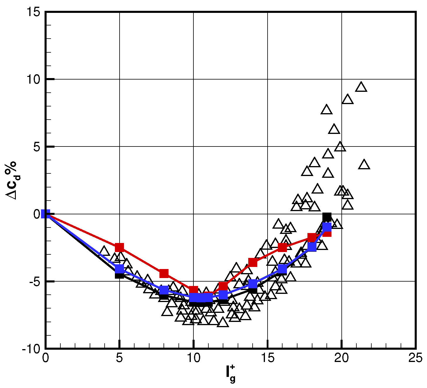
The performance of the two models in terms of drag reduction prediction are quite similar. Flat plate computations were performed on a grid with 640 cells in the streamwise direction and 256 cells in the normalwise direction, and 512 cells were distributed along the flat plate. In Figure 1 and Figure 2, the computed drag reduction applying Equations (6)–(9) is compared with the experiments and a DNS by García-Mayoral and Jiménez [33]. In particular, in Figure 2, the improvement obtained by adopting the new formulae is evident. Equation (9) can be easily adapted for the drag reduction prediction of a specific riblet shape. In Figure 3, the computed drag reduction in the case of blade riblets is compared with the experiments of Bechert et al. [7] showing a very good agreement.
Even if both models reproduce the drag reduction curve well, the -based model is simpler to apply to the drag increase regime, while the slip length model should have some kind of adaptation to obtain a drag increase. On the other hand, the slip length model is not linked to a turbulence model and can be adopted in an LES or DNS solver. A limitation of the -based model is that the values of needed to achieve a drag reduction of 6–8% are very large, and this may lead to lack of accuracy. Indeed, a different solver found a strong dependency of the drag reduction on grid until was reached. This is not surprising because the large values of at the wall imply strong gradients near the wall; thus, if the number of grid points inside the boundary layer is not sufficient, the gradient computation may be inaccurate. In Figure 4, a grid dependency study in the case of the flat plate flow is shown. The finest grid had 640 cells in the streamwise direction and 256 cells in the normalwise direction, 512 cells were distributed along the flat plate; the coarser grids were obtained by halving the number of grid cells. The coarser grid had ; it is evident that the slip length model was almost grid independent, while the -based model converged at the finest mesh size. However, it has been found that this effect is less evident in 3D simulation cases. It is also clear that this aspect limits the amount of drag reduction that can be predicted by the -based model, differently from the slip length model that can theoretically predict any percentage of drag reduction.
It is well known that the drag reduction due to the riblets depends on the Reynolds number; in [35], a theoretical analysis showed that there was an evident decay of riblet performance with the Reynolds number; however, the reduction in performance decreased with the Reynolds number. For instance, the decrease in drag reduction from the Reynolds number to was less than . Equation (8) has an explicit dependence on the Reynolds number, while in Equation (9), the dependence on the Reynolds number is implicit through riblet spacing s. The results of the flat plate computations reported in Figure 5 show that Equation (9) better reproduced the theoretical Reynolds number dependence.
3. Effect of Riblets on Form Drag and Shock Wave
It has been shown by experiments and theoretical analysis that the physical mechanism responsible for the drag reduction by riblets is local, and that the riblets act on friction drag. However, some experiments investigating the flow over a flat plate under an adverse pressure gradient showed an increased effectiveness of riblets [36], a result also confirmed by Large Eddy Simulations [37]. The increasing efficiency of riblets in airfoil flows has been measured in other experiments, where an additional drag reduction while increasing the angle of attack was found, implying an effect of the pressure distribution on riblet performance. A variation in the displacement thickness in the DNS computation of two different drag reduction techniques was reported in Stroh et al. [38]. The slip length concept was also applied in a DNS by Banchetti et al. [39] who analyzed the drag reduction over a curved wall, applied by streamwise-traveling waves of spanwise velocity. In this case, the authors also found a pressure drag reduction that improved the drag reduction performance. Very recently, Mollicone et al. [40] showed how superhydrophobic surfaces reduced form drag in bluff bodies. In [22], this effect was analyzed in detail, applying the slip length model previously described in a RANS solver. In [35], a more reliable analysis was carried out employing a resolved LES, which confirmed the results. The analyses provided a possible explanation for the increased performance of riblets in pressure gradient flows. It has been shown that riblets induce small but significant modifications of the pressure distribution, which tends towards the inviscid; this effect leads to a form drag reduction in addition to the well known friction drag reduction. Indeed, the log-law is not influenced by the pressure gradient; however, the boundary layer developed with the modified has a secondary influence on the outer inviscid flow and on the pressure distribution in particular, as is well known by Prandtl’s boundary layer theory. In Figure 6, the LES computation results show the effect of riblets on the pressure coefficient distribution along three different airfoils; it is evident that the pressure recovery at the trailing edge and the expansion peak are influenced by the riblets. A quantitative analysis with the help of the classical matched asymptotic expansion technique shows that the riblets reduce the displacement thickness of the boundary layer. The reduced thickness of the equivalent body leads to the form drag reduction. In Figure 7, the effect of the riblets on the displacement thickness is shown.
The significant influence of riblets on the location and strength of the shock waves was first observed in [16], where the -based model was applied to a transonic wing body configuration in the NASA Common Research Model (CRM). In Figure 8, the effect of the riblets on the shock wave of a wing section is shown. The effect of the riblets on the shock wave position and strength is evident. A deeper analysis of a typical transonic test case, the RAE 2822 case 9, showed that the riblets may induce a separation. In Figure 9, the pressure coefficient and skin friction coefficient show how the shock wave was stronger and moved downstream with the riblets installed also causing a shock-induced separation. A very recent DNS computation [41] confirmed the effect of the reduced skin friction on the shock wave strength and position due to a drag reduction device.
In the next sections, the effect of riblets on the form drag and shock wave of a full aircraft configuration will be shown.
4. Modeling the Riblet Effect on Aircraft Configuration
The boundary condition (6) was applied to full aircraft configurations in [16,17,18], showing how this model was able to analyze in detail riblet performance on practical aeronautical configurations. In particular, a transonic wing body configuration (NASA CRM) subject of the fifth AIAA CFD drag prediction workshop (DPW5) and two different wing body configurations designed to have a wide Natural Laminar Flow (NLF) along the wing were analyzed. In the case of the NASA CRM transonic configuration, the effect of the partial riblet installation was analyzed. The medium grid of DPW5 was used providing over the aircraft surface. In Figure 10, the lift drag polar curves with riblets installed on the wing, on the fuselage, and on both the wing and fuselage are shown. The analysis helps to evaluate the cost–benefit of riblet installation on single parts of the aircraft.
In the case of the NLF wing body, the effect of the riblets together with the NLF technology was considered. In Figure 11, the wing body configuration is shown with the pressure coefficient distribution on the body and the module of x-vorticity in the wake.
A structured mesh with 40 millions cells at the finest level was used. A grid convergence analysis while reducing the mesh size was first performed; in Figure 12, the computed polar curves for the three grid levels ( is the finest) shows that the medium grid (), with 20 millions cells, returned good accuracy, and it was used for the following calculations.
In Figure 13, the lift drag polar curves in the case of an NLF wing body with and without riblets are shown. The NLF conditions were obtained by imposing the transition line on the wing using data provided by the designers; the production terms of the turbulence model were set to zero in the laminar zone [42]. It is interesting to note that also in the case of NLF, riblet installation in the turbulent zones returned a significant additional drag reduction; indeed, in terms of drag reduction in cruise condition (), 29 drag counts were computed with NLF only against 40 drag counts with NLF and riblets. It must be remarked that the riblets were installed both on the wing and fuselage with constant . With this choice, the model could evaluate, as a result of the numerical simulation, the optimal riblet height distribution over the aircraft surface (Figure 14).
A drag breakdown by far-field methods [43,44] allowed the analysis of the effects of the riblets on the form drag and on the shock wave. In Figure 15 and Figure 16, the viscous drag breakdown showed that the reduction in form drag contributed to the total drag reduction, and that the decrease in the total drag reduction with the angle of attack was certainly due to the increase in induced drag on which the riblets did not act but also to the decrease in form drag reduction.
The strong increase in the form drag at a 4 degree of angle of attack was due also to the presence of a shock wave not present at the previous angles of attack. The analysis of the shock wave with and without riblets provides interesting details. In Figure 17, the shock wave zone is shown (the supersonic zone is in red). It can be noted that the supersonic zone in the case of NLF control and without NLF control with riblets was slightly wider with respect to the case without NLF and riblets (no flow control). The computed wave drag in the case of NLF control (21 drag counts) was substantially the same as that computed in the case of the fully turbulent flow with riblets (22 drag counts). This result shows that the effect of riblets on the shock wave was similar to the effect due to the NLF control and must be considered in the aircraft design phase.
5. Conclusions
Two models for riblet simulation were analyzed, and two new formulae for the slip length model were proposed. The new formulae returned a better characterization of riblet performance; in particular, the equation that linked the slip length to the riblet spacing ratio to better accounted for the Reynolds number dependence of the riblets’ performance. The comparison between the -based and slip length models showed a greater adaptability of the slip length model. The comparison with the experiments confirmed that both models reproduce the riblets’ performance in term of friction drag reduction in the whole range of well. The application of these models to complex flows allows a deep analysis of additional riblet effects, which had not been considered in previous experiments and theoretical analysis, such as the effect on the form drag and shock wave. It was shown that the application of riblets on the fuselage could be useful, and that riblets provide additional drag reduction when applied to the NLF configuration. The present analysis shows that, even if the drag reduction is modeled rather than effectively captured, these methods are very useful in providing insights into some unexpected effects of riblets.
Funding
This research received no external funding.
Conflicts of Interest
The author declares no conflict of interest.
References
- Spalart, P.R.; McLean, J.D. Drag reduction: Enticing turbulence, and then an industry. Philos. Trans. R. Soc. A 2011, 369, 1556–1569. [Google Scholar] [CrossRef] [Green Version]
- Martin, S.; Bhushan, B. Modeling and optimization of shark-inspired riblet geometries for low drag applications. J. Colloid Interface Sci. 2016, 474, 206–215. [Google Scholar] [CrossRef] [PubMed]
- Zhang, Y.; Chen, H.; Fu, S.; Dong, W. Numerical study of an airfoil with riblets installed based on large eddy simulation. Aerosp. Sci. Technol. 2018, 78, 661–670. [Google Scholar] [CrossRef]
- Choi, H.; Moin, P.; Kim, J. Direct Numerical Simulation of Turbulent Flow over Riblets. J. Fluid Mech. 1993, 255, 503–539. [Google Scholar] [CrossRef]
- El-Samni, O.; Chun, H.; Yoon, H. Drag reduction of turbulent flow over thin rectangular riblets. Int. J. Eng. Sci. 2007, 45, 436–454. [Google Scholar] [CrossRef]
- Walsh, M.J. Drag Characteristics of V-groove and Transverse Curvature Riblets. Prog. Astronaut. Aeronaut. 1980, 72, 168–184. [Google Scholar]
- Bechert, D.; Bruse, M.; Hage, W.; van der Hoeven, J.; Hoppe, G. Experiments on Drag-reducing Surfaces and their Optimization with an Adjustable Geometry. JFM 1997, 338, 59–87. [Google Scholar] [CrossRef]
- Choi, K. Near-wall structure of a turbulent boundary layer with riblets. J. Fluid Mech. 1989, 208, 417–458. [Google Scholar] [CrossRef]
- Lee, S.J.; Jang, Y. Control of Flow around a NACA 0012 Airfoil with a Micro-Riblet Film. J. Fluids Struct. 2005, 20, 659–672. [Google Scholar] [CrossRef]
- Hou, J.; Hokmabad, B.; Ghaemi, S. Three-dimensional measurement of turbulent flow over a riblet surface. Exp. Therm. Fluid Sci. 2017, 85, 229–239. [Google Scholar] [CrossRef]
- Luchini, P.; Manzo, F.; Pozzi, A. Resistance of Grooved Surface to Parallel Flow and Cross-flow. J. Fluid Mech. 1991, 228, 87–109. [Google Scholar] [CrossRef]
- Aupoix, B.; Pailhas, G.; Houdeville, R. Towards a General Strategy to Model Riblet Effects. AIAA J. 2012, 50, 708–716. [Google Scholar] [CrossRef]
- Koepplin, V.; Herbst, F.; Seume, J.R. Correlation-based riblet model for turbomachinery applications. J. Turbomach. 2017, 139. [Google Scholar] [CrossRef]
- Mele, B.; Tognaccini, R. Numerical simulation of riblets on airfoils and wings. In Proceedings of the 50th AIAA Aerospace Sciences Meeting including the New Horizons Forum and Aerospace Exposition, AIAA 2012-0861, Nashville, TN, USA, 9–12 January 2012. [Google Scholar] [CrossRef]
- Jiménez, J. Turbulent Flows over Rough Walls. Annu. Rev. Fluid Mech. 2004, 36, 173–196. [Google Scholar] [CrossRef]
- Mele, B.; Tognaccini, R.; Catalano, P. Performance assessment of a transonic wing-body configuration with riblets installed. J. Aircr. 2016, 53, 129–140. [Google Scholar] [CrossRef] [Green Version]
- Mele, B.; Russo, L.; Tognaccini, R. Drag bookkeeping on an aircraft with riblets and NLF control. Aerosp. Sci. Technol. 2020, 98, 105714. [Google Scholar] [CrossRef]
- Catalano, P.; de Rosa, D.; Mele, B.; Tognaccini, R.; Moens, F. Performance Improvements of a Regional Aircraft by Riblets and Natural Laminar Flow. J. Aircr. 2020, 57, 29–40. [Google Scholar] [CrossRef]
- Jiahe, L.; Yanming, L.; Jiang, W. Evaluation method of riblets effects and application on a missile surface. Aerosp. Sci. Technol. 2019, 95, 105418. [Google Scholar]
- Ran, W.; Zare, A.; Jovanovic, M. Model-based design of riblets for turbulent drag reduction. J. Fluid Mech. 2020, 906, 1–37. [Google Scholar] [CrossRef]
- Wang, L.; Wang, C.; Wang, S.; Sun, G.; You, B.; Hu, Y. A novel ANN-Based boundary strategy for modeling micro/nanopatterns on airfoil with improved aerodynamic performances. Aerosp. Sci. Technol. 2022, 121, 107347. [Google Scholar] [CrossRef]
- Mele, B.; Tognaccini, R. Slip length based boundary condition for modeling drag reduction devices. AIAA J. 2018, 56, 3478–3490. [Google Scholar] [CrossRef]
- Min, T.; Kim, J. Effects of hydrophobic surface on skin-friction drag. Phys. Fluids 2004, 16, L55. [Google Scholar] [CrossRef]
- Rastegari, A.; Akhavan, R. The common mechanism of turbulent skin-friction drag reduction with superhydrophobic longitudinal microgrooves and riblets. J. Fluid Mech. 2018, 838, 68–104. [Google Scholar] [CrossRef]
- Alinovi, E.; Bottaro, A. Apparent slip and drag reduction for the flow over superhydrophobic and lubricant-impregnated surfaces. Phys. Rev. Fluids 2018, 3, 124002. [Google Scholar] [CrossRef]
- Bottaro, A.; Naqvi, S. Effective boundary conditions at a rough wall: A high-order homogenization approach. Meccanica 2020, 55, 1781–1800. [Google Scholar] [CrossRef]
- Chang, J.; Jung, T.; Choi, H.; Kim, J. Predictions of the effective slip length and drag reduction with a lubricated micro-groove surface in a turbulent channel flow. J. Fluid Mech. 2019, 874, 797–820. [Google Scholar] [CrossRef]
- Zhang, Z.; Zhang, N.; Cai, C.; Kang, K. A General Model for the Riblet Simulation in Turbulent Flows. Int. J. Comput. Fluid Dyn. 2020, 34, 333–345. [Google Scholar] [CrossRef]
- Luchini, P. Linearized no-slip boundary conditions at a rough surface. J. Fluid Mech. 2013, 737, 349–367. [Google Scholar] [CrossRef] [Green Version]
- Wilcox, D.C. Turbulence Modeling for CFD-II Edition; DCW Industries: San Bernardino, CA, USA, 1998. [Google Scholar]
- Menter, F.R.; Egorov, Y. Two-Equation Eddy-Viscosity Turbulence Models for Engineering Applications. Flow Turbul. Combust. 2010, 85, 113–138. [Google Scholar] [CrossRef]
- Hirsch, C. The Numerical Computation of Internal and External Flows, Volumes 1, 2; John Wiley & Sons: Hoboken, NJ, USA, 1990. [Google Scholar]
- García-Mayoral, R.; Jiménez, J. Hydrodynamic Stability and Breakdown of the Viscous Regime over Riblets. J. Fluid Mech. 2011, 678, 317–347. [Google Scholar] [CrossRef]
- Saffman, P. A Model for Inhomogeneous Turbulent Flow. Proc. R. Soc. Lond. A 1970, 317, 417–433. [Google Scholar] [CrossRef]
- Mele, B.; Tognaccini, R.; Catalano, P.; de Rosa, D. Effect of body shape on riblets performance. Phys. Rev. Fluids 2020, 5, 124609. [Google Scholar] [CrossRef]
- Debisschop, J.; Nieuwstadt, F. Turbulent Boundary Layer in an Adverse Pressure Gradient: Effectiveness of Riblets. AIAA J. 1996, 34, 932–937. [Google Scholar] [CrossRef]
- Boomsma, A.; Sotiropoulos, F. Riblet drag reduction in mild adverse pressure gradient: A numerical investigation. Int. J. Heat Fluid Flow 2015, 56, 251–260. [Google Scholar] [CrossRef]
- Stroh, A.; Hasegawa, Y.; Schlatter, P.; Frohnapfel, B. Global effect of local skin friction drag reduction in spatially developing turbulent boundary layer. J. Fluid Mech. 2016, 805, 303–321. [Google Scholar] [CrossRef] [Green Version]
- Banchetti, J.; Luchini, P.; Quadrio, M. Turbulent Drag Reduction Over Curved Walls. J. Fluid Mech. 2020, 896, A10. [Google Scholar] [CrossRef]
- Mollicone, J.; Battista, F.; Gualtieri, P.; Casciola, C. Superhydrophobic surfaces to reduce form drag in turbulent separated flows. AIP Adv. 2022, 12, 075003. [Google Scholar] [CrossRef]
- Quadrio, M.; Chiarini, A.; Banchetti, J.; Gatti, D.; Memmolo, A.; Pirozzoli, S. Drag reduction on a transonic airfoil. J. Fluid Mech. 2022, 942, R2. [Google Scholar] [CrossRef]
- Catalano, P.; Mele, B.; Tognaccini, R. On the implementation of a turbulence model for low Reynolds number flows. Comput. Fluids 2015, 109, 67–71. [Google Scholar] [CrossRef]
- Paparone, L.; Tognaccini, R. Computational Fluid Dynamics-based drag prediction and decomposition. AIAA J. 2003, 41, 1647–1657. [Google Scholar] [CrossRef] [Green Version]
- Lanzetta, M.; Mele, B.; Tognaccini, R. Advances in aerodynamic drag extraction by far field methods. J. Aircr. 2015, 52, 1873–1886. [Google Scholar] [CrossRef]

Figure 2.
Computed drag reduction vs. . Red: Equation from [22], blue: Equation (8), black: Equation (9) ∆: experiment [7].


Figure 6.
LES averaged pressure coefficients. (a): NACA 0015, , ; (b): NACA 0012, , ; (c): EPPLER 387, , . ![Fluids 07 00249 i001]() : riblets off,
: riblets off, ![Fluids 07 00249 i002]() : riblets on.
: riblets on.
 : riblets off,
  : riblets on.
Figure 6.
LES averaged pressure coefficients. (a): NACA 0015, , ; (b): NACA 0012, , ; (c): EPPLER 387, , . ![Fluids 07 00249 i001]() : riblets off,
: riblets off, ![Fluids 07 00249 i002]() : riblets on.
: riblets on.
: riblets off, : riblets on.
Figure 7.
Effect of riblets on the displacement thickness on the airfoil suction side [35]. (a): NACA 0015, , ; (b): NACA 0012, , ; (c): EPPLER 387, , . ![Fluids 07 00249 i001]() : riblets off,
: riblets off, ![Fluids 07 00249 i002]() : riblets on.
: riblets on.
: riblets off, : riblets on.
Figure 7.
Effect of riblets on the displacement thickness on the airfoil suction side [35]. (a): NACA 0015, , ; (b): NACA 0012, , ; (c): EPPLER 387, , . ![Fluids 07 00249 i001]() : riblets off,
: riblets off, ![Fluids 07 00249 i002]() : riblets on.
: riblets on.
: riblets off, : riblets on.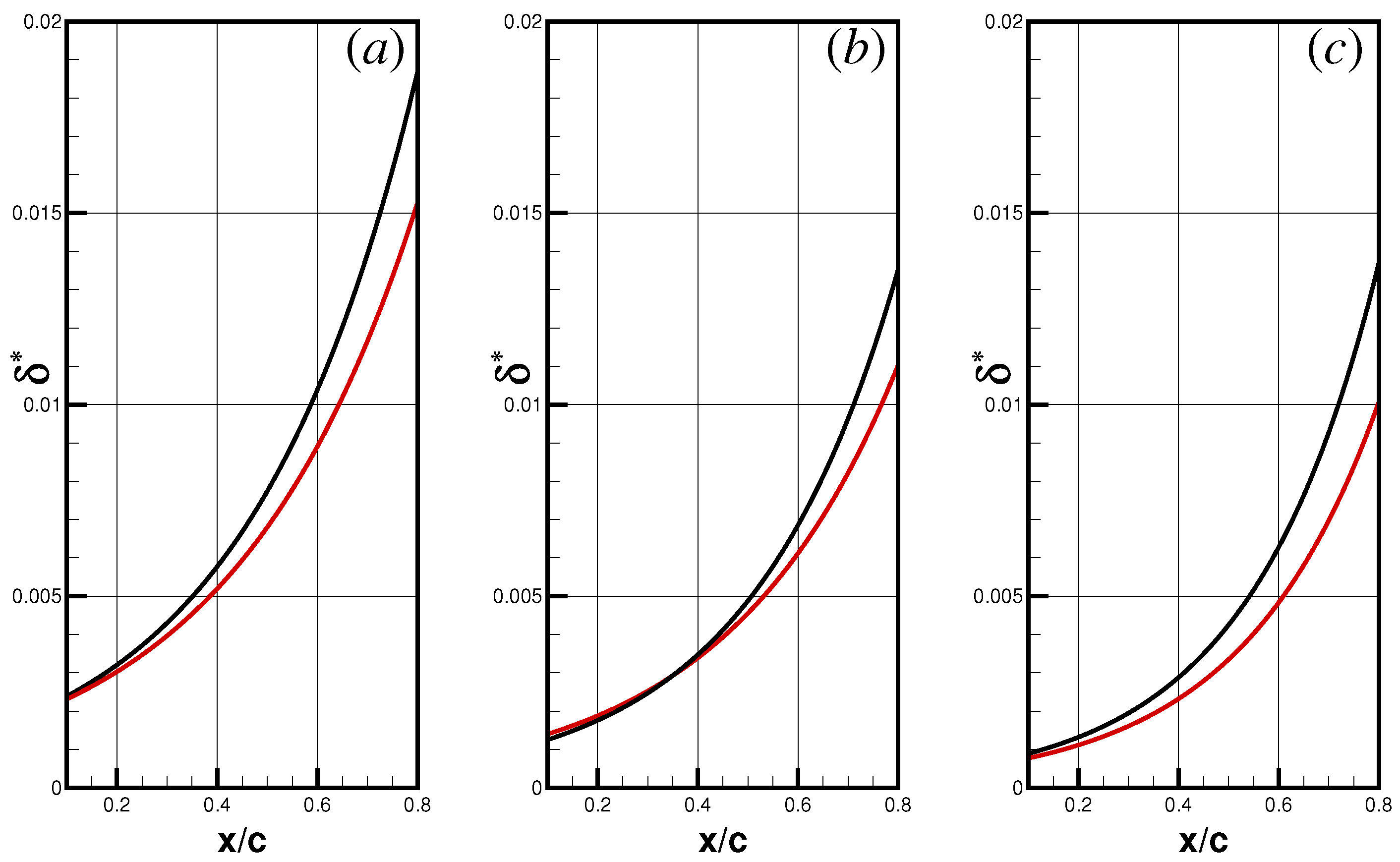
Figure 8.
NASA CRM wing body configuration: , , , . Effect of riblets on shock wave [16].
Figure 8.
NASA CRM wing body configuration: , , , . Effect of riblets on shock wave [16].
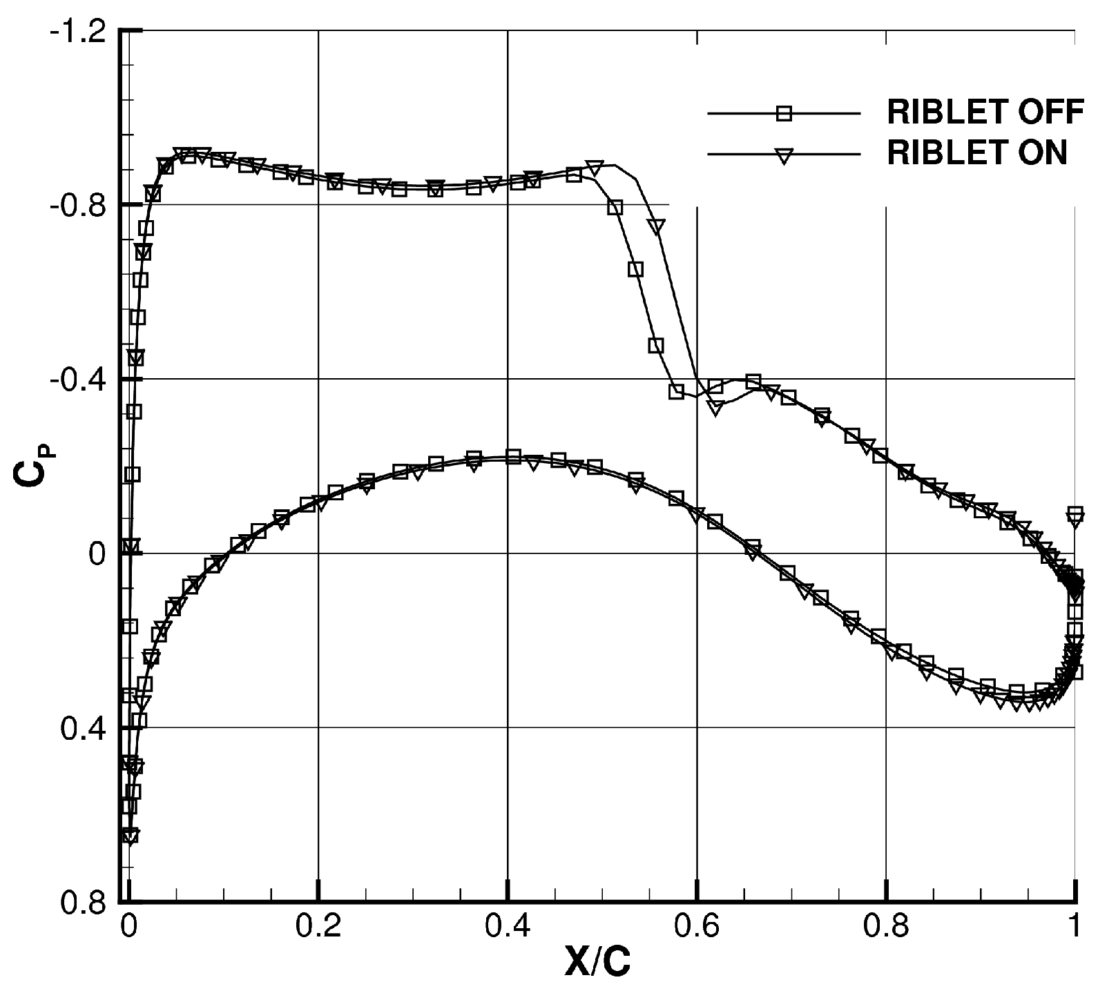
Figure 9.
RAE 2822 airfoil: , , . (a) Pressure coefficient; (b) skin friction coefficient [16].
Figure 9.
RAE 2822 airfoil: , , . (a) Pressure coefficient; (b) skin friction coefficient [16].
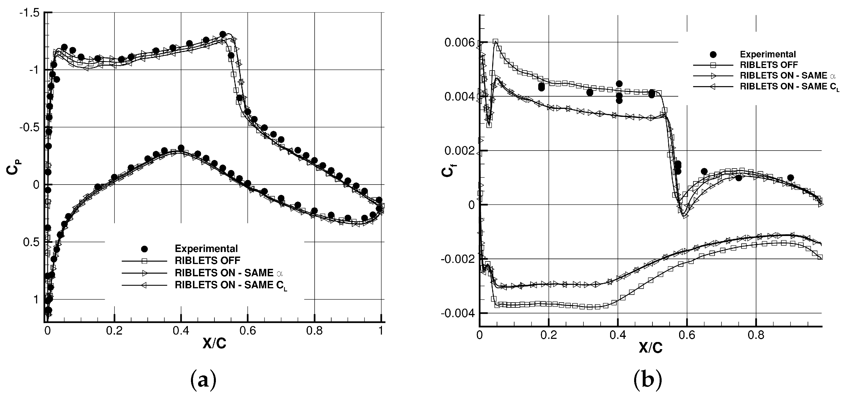
Figure 10.
NASA CRM wing body configuration: , . Lift drag polar curves [16].
Figure 10.
NASA CRM wing body configuration: , . Lift drag polar curves [16].
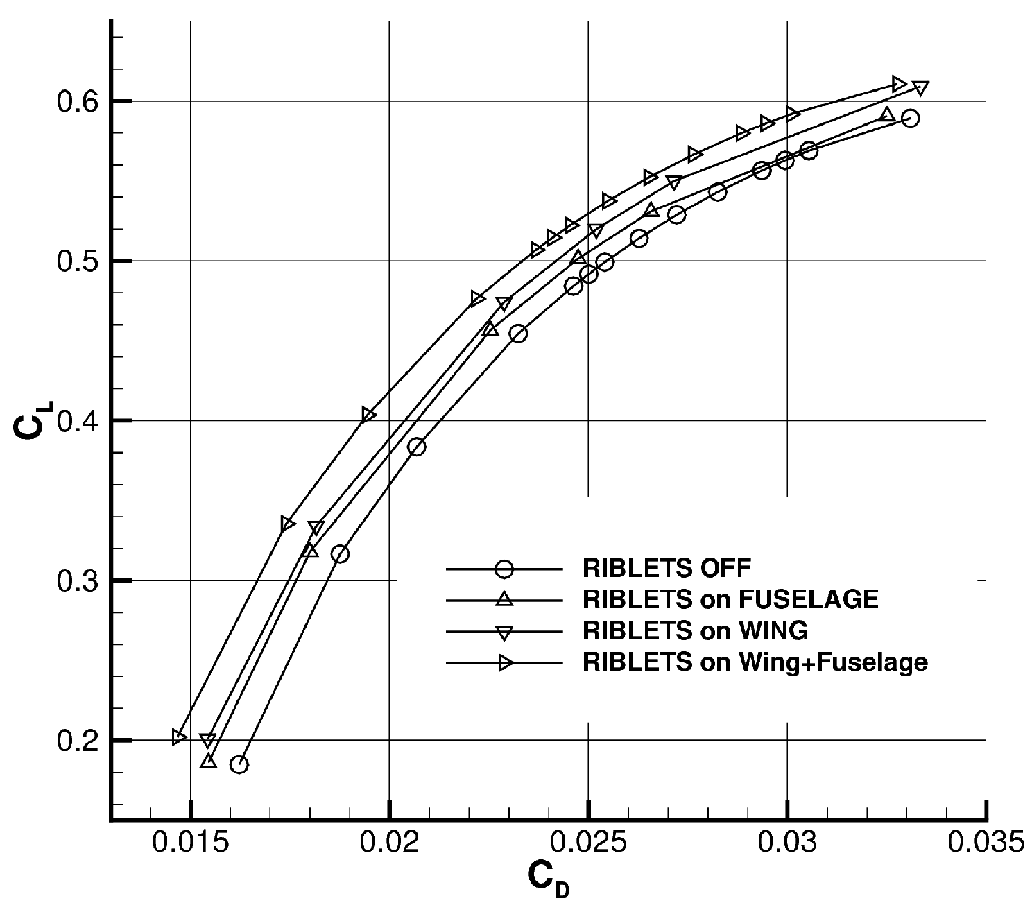
Figure 11.
Wing body: , , . Pressure coefficient distribution and x-vorticity module in the wake [35].
Figure 11.
Wing body: , , . Pressure coefficient distribution and x-vorticity module in the wake [35].
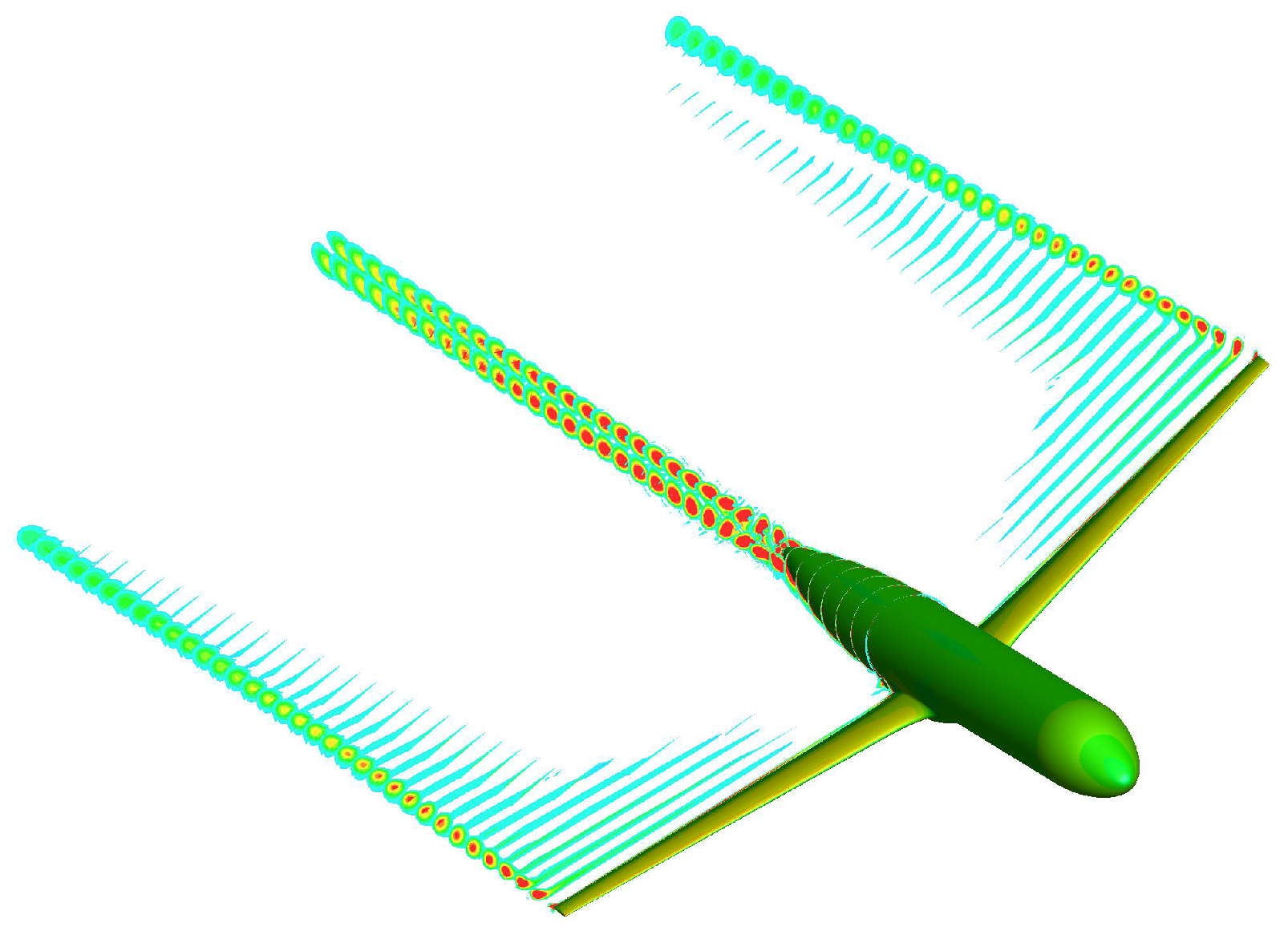
Figure 12.
NLF wing body configuration: , . Lift-drag polar curves obtained on three grid levels [35].
Figure 12.
NLF wing body configuration: , . Lift-drag polar curves obtained on three grid levels [35].
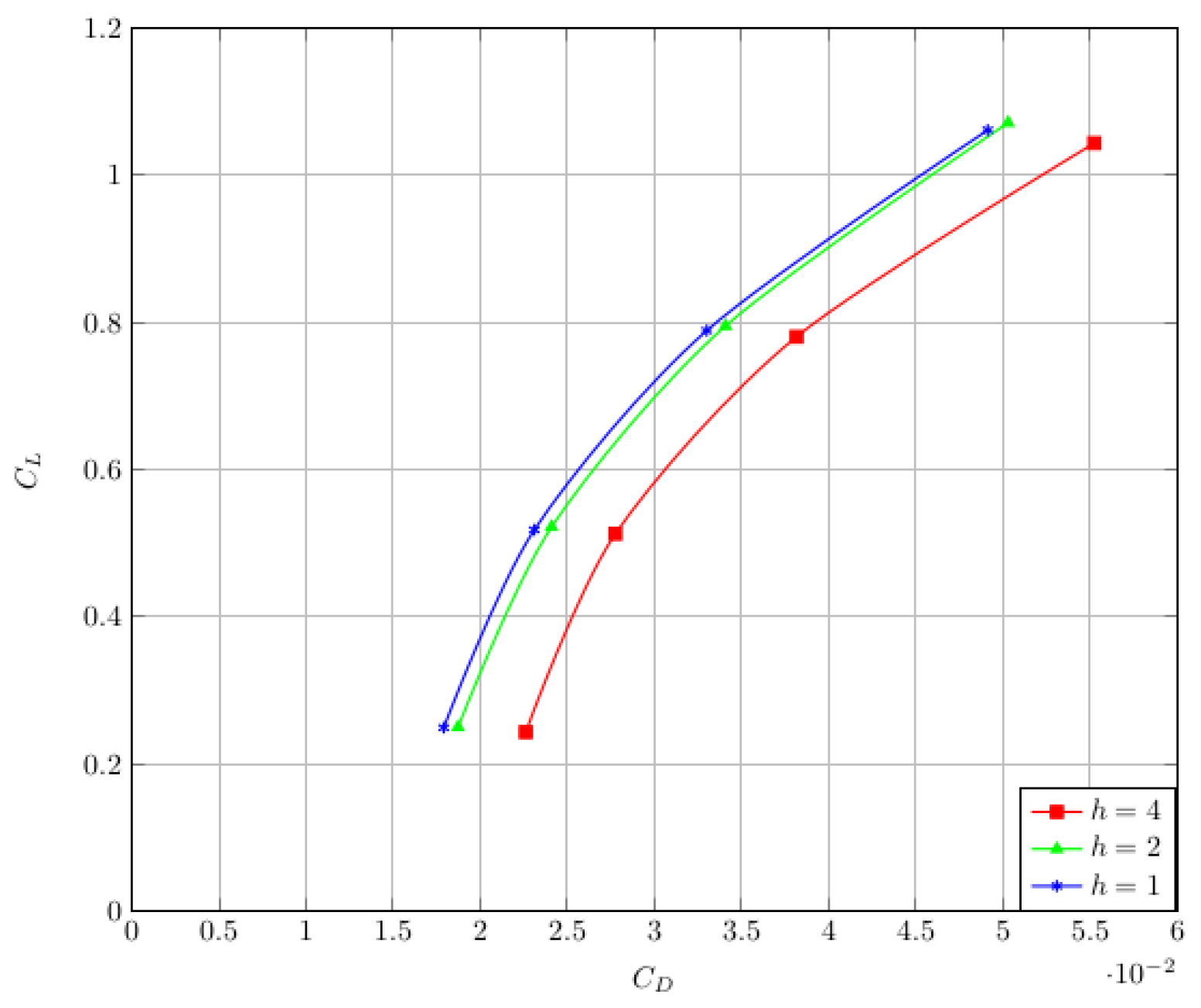
Figure 13.
NLF wing body configuration: , . Lift drag polar curves with and without riblets [35].
Figure 13.
NLF wing body configuration: , . Lift drag polar curves with and without riblets [35].

Figure 14.
NLF wing body: , , . Computed optimal riblet height distribution (symmetric sawtooth riblets). (a) Upper skin, (b) lower skin [35].
Figure 14.
NLF wing body: , , . Computed optimal riblet height distribution (symmetric sawtooth riblets). (a) Upper skin, (b) lower skin [35].

Figure 15.
NLF wing body, , . Viscous drag breakdown with NLF and riblets [35].
Figure 15.
NLF wing body, , . Viscous drag breakdown with NLF and riblets [35].
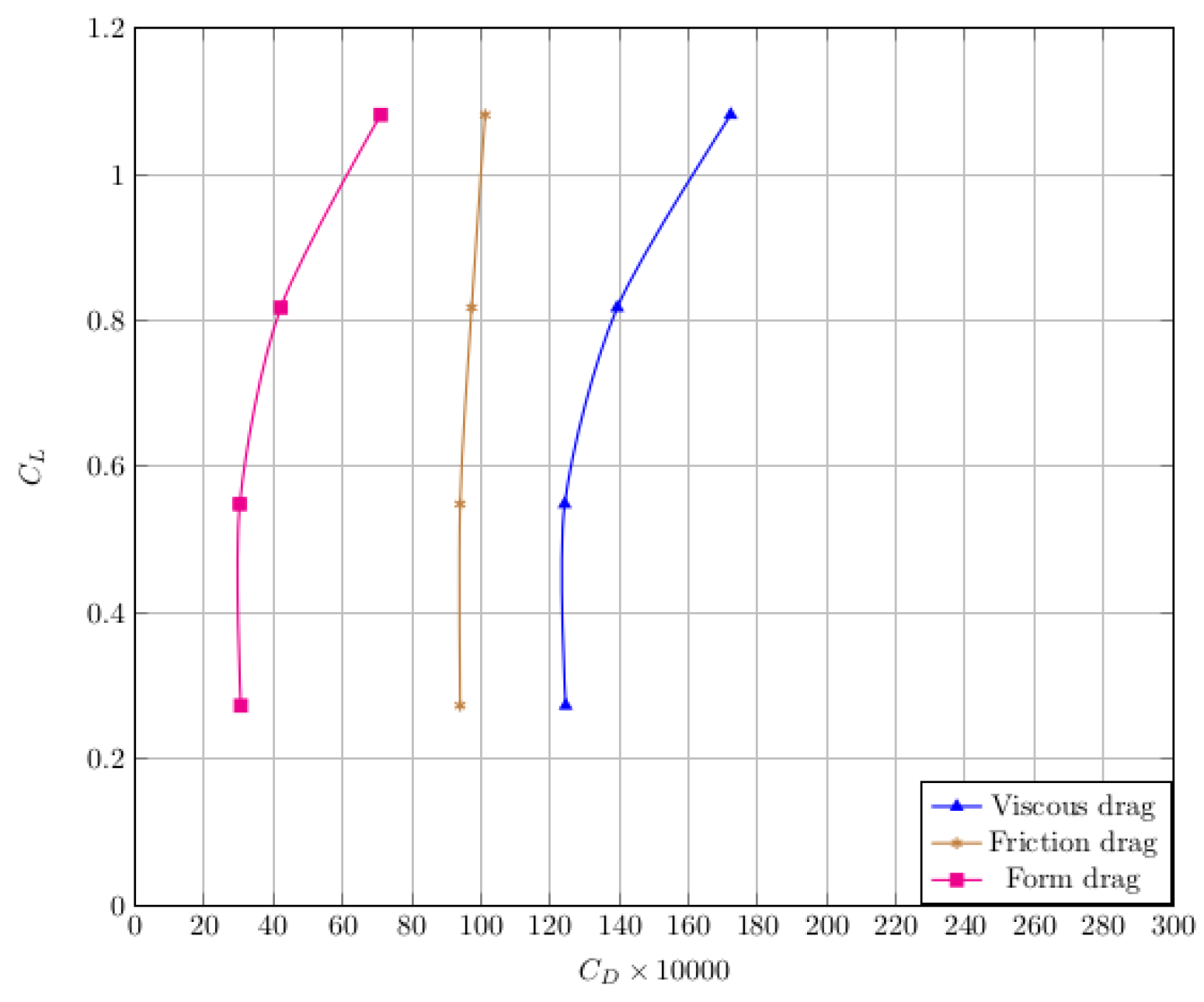
Figure 16.
NLF wing body, , . Drag reduction due to riblets vs. angle of attack [35].
Figure 16.
NLF wing body, , . Drag reduction due to riblets vs. angle of attack [35].
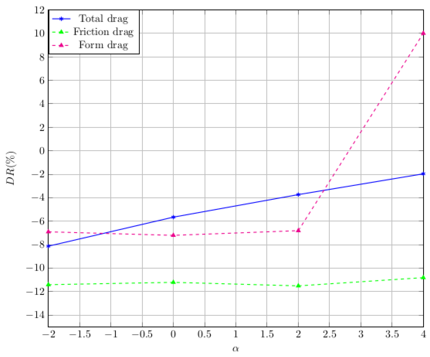
Figure 17.
Wing section of NLF wing body: , , . Visualization of the shock wave at wing section (supersonic zone in red). Top: NLF without riblets, middle: turbulent without riblets (no flow control), bottom: turbulent with riblets [35].
Figure 17.
Wing section of NLF wing body: , , . Visualization of the shock wave at wing section (supersonic zone in red). Top: NLF without riblets, middle: turbulent without riblets (no flow control), bottom: turbulent with riblets [35].

Publisher’s Note: MDPI stays neutral with regard to jurisdictional claims in published maps and institutional affiliations. |
© 2022 by the author. Licensee MDPI, Basel, Switzerland. This article is an open access article distributed under the terms and conditions of the Creative Commons Attribution (CC BY) license (https://creativecommons.org/licenses/by/4.0/).
Share and Cite
MDPI and ACS Style
Mele, B. Riblet Drag Reduction Modeling and Simulation. Fluids 2022, 7, 249. https://doi.org/10.3390/fluids7070249
AMA Style
Mele B. Riblet Drag Reduction Modeling and Simulation. Fluids. 2022; 7(7):249. https://doi.org/10.3390/fluids7070249
Chicago/Turabian StyleMele, Benedetto. 2022. "Riblet Drag Reduction Modeling and Simulation" Fluids 7, no. 7: 249. https://doi.org/10.3390/fluids7070249