
A Mathematical Model of Blood Loss during Renal Resection


1
Department of Biomedical Engineering, University of Strathclyde, Glasgow G4 0NW, UK
2
Centre for Precision Manufacturing—Department of Design Manufacturing & Engineering Management, University of Strathclyde, Glasgow G1 1XJ, UK
3
Department of Surgery, University of Cambridge, Cambridge CB2 0QQ, UK
*
Authors to whom correspondence should be addressed.
Fluids 2023, 8(12), 316; https://doi.org/10.3390/fluids8120316
Submission received: 10 November 2023
/
Revised: 1 December 2023
/
Accepted: 7 December 2023
/
Published: 10 December 2023
(This article belongs to the Section Mathematical and Computational Fluid Mechanics)
Abstract
:In 2021, approximately 51% of patients diagnosed with kidney tumors underwent surgical resections. One possible way to reduce complications from surgery is to minimise the associated blood loss, which, in the case of partial nephrectomy, is caused by the inadequate repair of branching arteries within the kidney cut during the tumor resection. The kidney vasculature is particularly complicated in nature, consisting of various interconnecting blood vessels and numerous bifurcation, trifurcation, tetrafurcation, and pentafurcation points. In this study, we present a mathematical lumped-parameter model of a whole kidney, assuming a non-Newtonian Carreau fluid, as a first approximation of estimating the blood loss arising from the cutting of single or multiple vessels. It shows that severing one or more blood vessels from the kidney vasculature results in a redistribution of the blood flow rates and pressures to the unaltered section of the kidney. The model can account for the change in the total impedance of the vascular network and considers a variety of multiple cuts. Calculating the blood loss for numerous combinations of arterial cuts allows us to identify the appropriate surgical protocols required to minimise blood loss during partial nephrectomy as well as enhance our understanding of perfusion and account for the possibility of cellular necrosis. This model may help renal surgeons during partial organ resection in assessing whether the remaining vascularisation is sufficient to support organ viability.
1. Introduction
Surgery is the treatment most likely to cure patients [1]. Data from 2004 to 2014 [2] suggest that there was a 27% increase in surgery, with over 10 million operations being performed [3]. In 2020, due to COVID-19, over 1.5 million surgical procedures were cancelled in England and Wales, representing, approximately, a 35% reduction [4]. Due to COVID-19, the waiting lists for cancer surgery grew substantially, possibly leading to more deaths. Approximately 51% of patients diagnosed with kidney tumors underwent surgical resections in 2021 [5]. The economic cost of surgery in the UK was approximately GBP 55 billion between 2009 and 2014 (approximately GBP 10.9 billion per annum) which amounts to 9.4% of the total NHS budget (GBP 117 billion, 2013–2014) [6]. Complications, such as bleeding during surgery, are an important risk to patients and put surgeons under constant pressure [7,8,9].
An example of an operation with a high bleeding risk is partial nephrectomy for the treatment of kidney tumors, due to cutting into the organ to excise the tumor before repairing it with sutures. Jaramillo et al. [9] highlight the necessity of developing more accurate methods to both estimate and measure blood loss and emphasise the limitations and inaccuracies of direct measurements. Clinical findings by Rosiello et al. [10] have shown that excessive blood loss puts a patient at risk of chronic kidney disease. Anatomically, the renal vasculature is particularly complex in structure and morphology, consisting of many blood vessels connected via multiple bifurcation, trifurcation, tetrafurcation, and pentafurcation points. The kidney has been successfully imaged by Puelles et al. [11] via optical projection tomography and Schutter et al. [12] via MRI, while Nordsletten et al. [13] proposed an automated segmentation technique for reconstruction from μCT images. A comprehensive understanding of blood flow within the kidney vasculature can enhance the efficacy of renal surgery and the precision of targeted localised drug delivery, such as the use of drug-loaded ultrasound contrast agent microbubbles alongside high-frequency ultrasound [14,15]. A typical healthy human kidney has blood flow rates of 600 mL/min [16], with both kidneys requiring roughly 20% of an average adult’s cardiovascular blood output. In a partial nephrectomy, the main renal artery of the kidney is usually clamped to excise the tumor and repair the kidney with sutures; therefore, an estimation of the possible blood loss percentage during renal surgery is of high importance for the surgeon. There are several studies that highlight a link between general surgery and chronic kidney disease [17,18,19,20,21].
Several existing works have contributed to the understanding of renal haemodynamics and blood flow autoregulation [22,23,24,25,26,27,28,29,30,31,32,33,34,35,36,37], as well as stenosis in human or animal kidney models. For example, Sgouralis and Layton [38], Postnov et al. [39], Cury et al. [40], and Deng and Tsubota [41,42] offered key insights into healthy renal haemodynamics using various numerical modelling approaches. Specifically, Postnov et al. [39] used a probability-based topological approach to develop a mathematical model of a kidney arterial network. Cury et al. [40] developed a computational model of the kidney arterial structure. Mathematical approximations for renal blood flow autoregulation were developed by Holstein-Rathlon and Marsh [43] and Sgouralis et al. [44]. Important contributions to the appreciation of renal stenosis were made by Hao et al. [45] via mathematical modelling. Basri et al. [46] developed a computational model to simulate the blood flow behavior in the abdominal aorta. There are a large number of other previous works focusing on the computational and mathematical modelling of various arterial networks [47,48,49,50,51,52,53,54,55]. Furthermore, several numerical approaches were previously tested in a wide range of arterial geometries [56,57,58,59,60,61,62,63]. Clinical research in the field of renal blood loss was conducted in recent years by Rosiello et al. [10]. However, none of these studies have considered the cutting of blood vessels as a result of surgery and its impact on the haemodynamics of the remaining kidney vasculature.
The novelty of this work lies in the near-real-time estimation of blood loss for single-, double-, and cross-vessel cuts for a complex extended renal vasculature. The presented simplified mathematical lumped-parameter model calculates, fast and reliably, the percentage of blood loss arising as an immediate effect of severed vessels during the partial nephrectomy of an asymmetric whole-kidney vascular network and prior to autoregulation recovery. This tool can be translated into the clinic and be personalised for specific patients. It can assist renal surgeons in evaluating the sufficiency of the remaining vascularisation to support organ viability during partial nephrectomy, thus allowing the best decision to be made for each individual patient. Furthermore, this study can offer a theoretical framework for assessing the adequacy of vascularisation in functional tissue engineering, drug development, and surgical planning applications.
The remainder of this article consists of a Methods section explaining the mathematical model, a Results section presenting calculations both schematically and in a tabular form, and a Discussion section, which considers the implications of the results and their potential impact on renal surgery. The limitations of the presented model and future work are also discussed.
2. Materials and Methods
In the following sections, we present a mathematical lumped-parameter model of the renal vasculature and an estimation of blood loss during partial nephrectomy. First, we describe the complex arterial network of a single kidney with 25 vascular nodes (Section 2.1, Figure 1); then, we discuss the numerical approximations made in this study (Section 2.2); in Section 2.3, we conduct a sensitivity analysis on a parent–daughter bifurcation to investigate the effects of the fluid model assumption; in Section 2.4, we provide details on model verification and validation; and, lastly, we explain the modelling of vessel cuts (Section 2.5).
2.1. Generating the Renal Vasculature
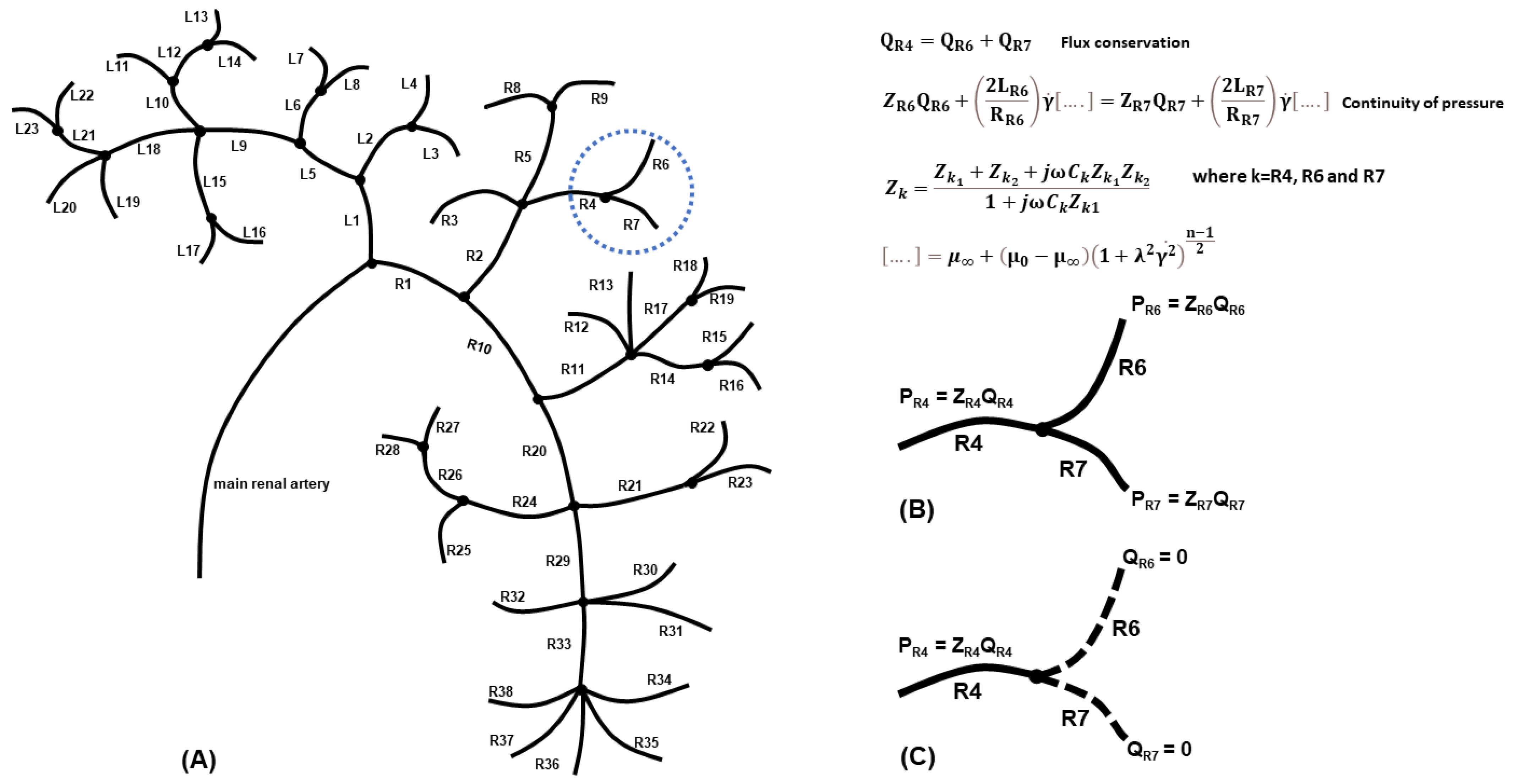
The optical projection tomography image procured by Puelles et al. [11] was our template for generating the geometry of a complex whole-kidney vascular network (Figure 1A). The asymmetric network consisted of 25 vascular nodes (including bifurcations, trifurcations, tetrafurcations, and pentafurcations, portrayed in Figure 1A as black circles) and 61 individual blood vessels (represented as line segments), organised in left and right branches according to the first bifurcation node of the main renal artery to the two primary daughter vessels, L1 and R1. The labelling of the vessels, respectively, on the left and right sides, started at the first node and continued following the vessel segments downstream towards the periphery. Hence, the whole-kidney network was comprised of 10 vascular nodes and 23 blood vessels (L1–L23) on the left side and 14 nodes and 38 vessels on the right side (R1–R38), in addition to the first node. The main daughter vessels’ radii (L1, R1) were calculated using Murray’s law [64], while the remaining vessel radii (L2–L23, R2–R38) were given values previously used by Cury et al. [40]. We could not apply the splitting method [65] in this work because the daughter/sub-daughter blood flux ratios for each individual branching node were unknown. Since the blood vessels were of a similar order of magnitude in length, for the purposes of simplicity, all blood vessels were assumed equal in length, like in the model of Cury et al. [40]. We also assumed that the vessels were cylindrical, with a constant cross-section (i.e., neglecting arterial tapering), and that the angle and 3D orientation were negligible, based on a previous study showing that the blood flow rate in a 1D model was not influenced by the angular orientation of each node [66].
2.2. Numerical Approximations
Several assumptions were made to model the flow in the vascular network of Figure 1A. (a) The flow was considered laminar and steady, governed by the flow equations for the conservation of flux and the continuity of pressure at each branching node. Taking as an example the bifurcation of vessel R4 to vessels R6 and R7 (Figure 1B), then, for each node, we solved a system of linear equations, such as
where Qk (here k = R4, R6, R7) is the vessel flux, ΔPk (here k = R6, R7) is the pressure gradient, and Pk is the pressure obtained from Ohm’s Law Pk = ZkQk, with Zk being the vessel impedance.
(b) The blood was assumed as an incompressible non-Newtonian fluid, following the Carreau fluid model [67], which accounts for the shear thinning effects. The Carreau model is given by the equation.
where µ0 and µ∞ represent the viscosities at the respective physical boundaries, and n is a non-dimensional number obtained empirically. The terms λ and represent the relaxation term and the shear strain rate, respectively. The shear strain rate for a typical unblocked artery is = 600 s−1, the relaxation time is λ = 3.313 s, µ0 = 0.056 Pas, µ∞ = 0.00345 Pas, and n = 0.3568 [67]. Applying the conservation of flux and the continuity of pressure at the example bifurcation point to vessels R6 and R7 (Figure 1B) results in a system of equations with
Using the conservation of flux Equation (1) and Equation (4) and rearranging yields
(c) Blood pulsation was not included since the flow behavior in small vessels can be approximated using the quasi-steady solution [68]. (d) The backflow associated with the pulse wave propagation within the vasculature was assumed small enough to be negligible. (e) The inlet blood flow rate at the main renal artery was taken equal to 600 mL/min [16]. (f) A physiological value of haematocrit was considered [69]. (g) The blood vessel walls were rigid and, for simplicity, due to the complexity and scale of the kidney vasculature, the non-linear viscoelastic characteristics of the vessel walls were negated. (h) We assumed that the simulated vessel cuts resulted in zero blood flow and, therefore, zero blood pressure. The outlet blood vessels that still connected to the vascular network had a constant pressure, given by Ohm’s Law (Figure 1C). (i) The impedance Zk of each blood vessel of the vasculature of Figure 1A (k = L1,…L23, R1,…R38) was determined using the three-element Windkessel model [50], comprised of a resistor Zk1 in parallel with a capacitor Ck, and both in series with another resistor Zk2. The capacitor represents the compliance of a blood vessel, given by
where ∆Vk is the difference in volume. The pressure Pk can be expressed as a function of the time t and the angular frequency ω, where P0 is the amplitude of the pressure, such that
Using Equations (6) and (7), the vessel flux, Qk, is given by
where j2 = −1, ω = 2πf, and f is the frequency. The impedance associated with the compliance, represented by ZCk, is written as
Using Equation (9) and applying basic circuit theory, we take
The modulus of Equation (10) provides the magnitude of the total impedance of each blood vessel (where k = L1, … L23, R1, … R38).
2.3. Effect of the Fluid Model Assumption on a Single-Node Asymmetric Bifurcation
In order to investigate the effect of the fluid model assumed on the calculated blood flux and pressure for each blood vessel in the complex kidney vasculature, we conducted a sensitivity analysis on a simple asymmetric parent–daughter bifurcation with a single vascular node (Figure S1 of Supplementary Material). For that, we used the Hagen–Poiseuille model with haematocrit, without and with backflow (Section S1.1, Section S1.2, respectively), a power law fluid model (Section S1.3) and the Carreau model (Section S1.4), which accounts for the non-Newtonian shear thinning behaviour of blood [67,70]. The radii, lengths, and impedances values used in this bifurcation are physiologically correct (Table S1), characteristic of a healthy kidney [40,71,72,73]. The physical parameters for the Carreau and the power law models are from Bessonov et al. [67] and Sochi [70], respectively.
The data from this sensitivity analysis illustrate that the effects of backflow (Qreflection) were so small as to be negligible, being approximately 1.4% of the total flux. There was little difference between the flow rates for the Hagen–Poiseuille fluid model with a constant viscosity, the power law, and the Carreau model. It is worth noting that the Carreau model is dependent on the shear strain rate, which influences the viscosity of blood, with higher shear strain rates resulting in a lower blood viscosity. Therefore, we primarily focused on the Carreau model without backflow when calculating the blood fluxes and blood losses that arise from the kidney vasculature in Figure 1A. Focusing on the Carreau model rather than the Newtonian model offers more flexibility since it allows us to account for shear thinning effects and varying shear rates.
2.4. Modelling Vessel Cuts
Since there were 61 individual blood vessels in the network in Figure 1A, there were potentially an equal number of vessels which could be cut and thousands of potential multiple-vessel cuts. Each cut has a unique, distinct set of equations that describe the conservation of flux and the continuity of pressure at each of the respective nodes. The schematic of Figure 1C represents an example of two severed blood vessels (R6 and R7) resulting in zero blood flow and zero blood pressure. The outlet blood vessel (R4) that still connected to the vascular network had a constant pressure, given by Ohm’s Law. To model the 61 single cuts, we had to construct an equivalent number of different sets of algorithms to determine the blood loss, blood flow, and blood pressure within the altered vascular network. Each unique set of equations consisted of numerous linear equations with unknown fluxes and pressures, which we determined numerically via the symbolic computing platform Mathematica© (v. 13.0) [74]. Developing all 61 separate and distinct sets of algorithms means that the presented blood loss model can account for the change in the total impedance of the vascular network system arising due to the severing and extraction of a particular blood vessel.
Since there were potentially thousands of possible combinations of cutting two or more vessels, in this study, we focused on the most significant multiple cuts, placing emphasis on the internal primary vessels within the kidney vasculature model. This was because the primary internal vessels within the vascular network exhibited the greatest blood flow rates due to their smaller impedances and larger radii and would, therefore, highlight the greatest blood losses and largest differences in blood flow rates and blood pressures. The severing of multiple vessels resulted in a new set of linear equations that accounted for the total change in impedance within the network. These were also solved numerically via Mathematica© to determine the blood losses from each of the severed vessels as well as to evaluate the blood flow and pressures in the remaining unsevered vessels. We were able to validate and confirm computationally that the blood flux at each bifurcation/trifurcation/tetrafurcation and pentafurcation node was always conserved.
2.5. Model Validation and Verification
Validation of our methodological modelling approach was conducted through comparing our calculations with the experimental findings of Zhao and Lieber [75] and Shroter and Sudlow [76] for a Y junction in the bifurcation plane, using the same physical parameters. Differences of 3.4% and 3.6% were found, respectively, for each study, demonstrating the suitability of our lumped-parameter mathematical model to predict experimental results. We further validated our model in the entire network of Figure 1A against the work of Jaramillo et al. [9], who studied one hundred patients undergoing urological surgery, measuring mass blood loss and blood volume loss under controlled conditions. Jaramillo et al. [9] highlighted the inaccuracy and unreliability of direct blood volume loss measurements and used three formulae in their study in order to provide the most accurate estimation of blood volume loss. A typically healthy patient had a mean blood volume loss of 3.64% (mean 198.2 mL based on a cardiac output of 5448 mL) using the Lόpez-Picado formula [77], which has shown agreement with directly measured blood loss, while we have calculated a blood volume loss of 2.46%, as a result of cutting the QR2 and QR10 blood vessels.
We also validated our model on both Y- and T-junction geometries based on those studied by Boumpouli et al. [56] for the pulmonary arteries, using the same physical dimensions and flow conditions. The mathematical model’s predictions were in good agreement with the flow rates and pressures found by Boumpouli et al. [56], who used a well-validated open source CFD code (OpenFOAM) for their flow analysis, with a difference of 1.1% and 1.6%, respectively, for the Y and T junction. This verifies the minimal influence of both varying branching angles and the inclusion of time evolution in the modelling process.
Using a simple Y bifurcation model (Figure S1A), we further explored the parameter space for the daughter vessel radius, the branch length, the haematocrit, the shear rate, and the impedance of the branching vessel (Tables S1 and S2; see Supplementary Material for the full range of parameter values examined). Changing the radius RL1 from 2.5 × 10⁻³ m to 1 × 10⁻³ m altered the daughter flux QL1 by 0.3%, whereas varying the length LL1 from 4 × 10⁻² m to 5 × 10⁻³ m changed the flux QL1 by 0.2%, indicating that both the length and radii have very little effect on the flux calculation. Similarly, altering the haematocrit from 0.40 to 0.55 changed QL1 by 0.05%. Changing the shear rate from 600 s−1 to 10,000 s−1 altered QL1 by 1.3%, suggesting that the model has a very small dependency on viscosity. We also explored the parameter space for the impedance of a daughter vessel by changing ZL1 from 3.3 × 10⁹ kgm−4s−1 to 4 × 10⁹ kgm−4s−1, which represents a 21.2% change, and found that the flux QL1 changed by 9.6%, implying that the single-node Y bifurcation model is more susceptible to small variations in the impedance since it has only two outputs. However, testing the effect of the impedance on the entire network of Figure 1A, using the same value percentage change, resulted in only 0.9% difference in QL1. This is because of the scale and structure of the complex vascular network studied consisted of multiple parallel branches (61 vessels and 25 vascular nodes), which makes it much less dependent on the impedance of the primary daughter vessel.
As discussed by Black et al. [62], the impedance and other Windkessel parameters may indeed require an iterative calibration when applied to specific patients, which is a challenging problem on its own for the small renal vessels. Future advances in high-resolution 4D flow MRI with improved velocity-to-noise levels may allow more detailed in vivo patient-specific flow measurements of the renal vasculature that can facilitate accurate calibration of the Windkessel parameters.
To allow transparency and reproducibility for the presented model, we have added the in-house Mathematica® scripts focussing on the healthy kidney, a cross-sectional cut to vessels QL18 and QR33, and a kidney resection at QL1 to the open source database of the University of Strathclyde (https://doi.org/10.15129/78fb70eb-0e8d-4a11-9d6d-97b050266743, made available on 29 November 2023).
3. Results
We present, first, the flow rate and pressure distributions in a healthy (uncut) asymmetric whole-kidney vascular network (Section 3.1) and, subsequently, the possible blood loss arising from various cases of partial nephrectomy (Section 3.2, Section 3.3 and Section 3.4).
3.1. Modelling the Healthy (Uncut) Kidney Vascular Network
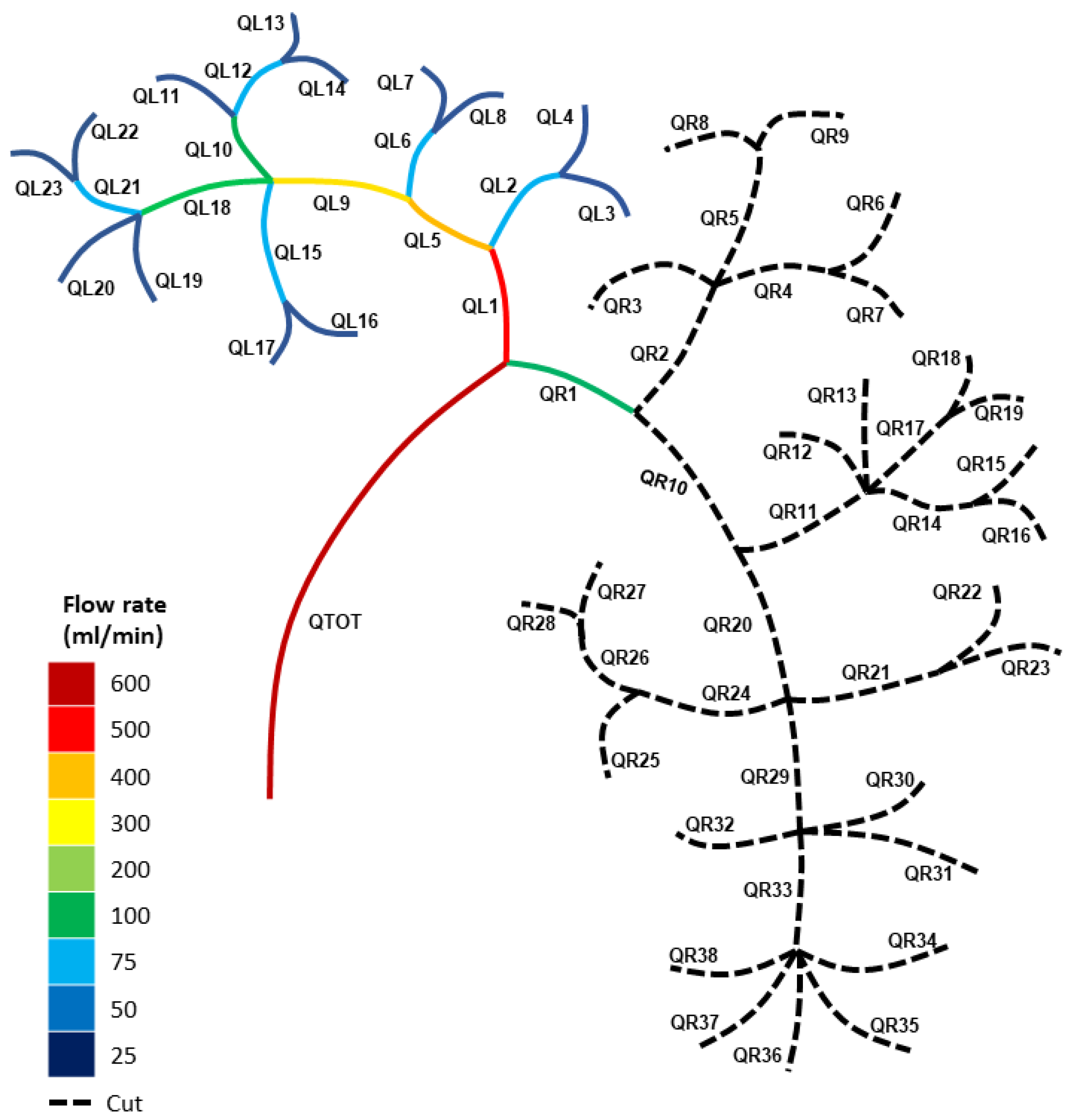
Before we consider modelling the blood loss from both single- and double-vessel cuts, we modelled the blood flow in a typical healthy vascular network. Using the Carreau fluid model denoted by Equation (3), alongside the conservation of flux and the continuity of pressure at each bifurcation/trifurcation/tetrafurcation and pentafurcation node (Equations (1) and (4)), we calculated the blood fluxes through the healthy (uncut) vasculature represented by Figure 1A, using the physical data from Table 1 and Table 2. The calculations for each individual vessel are displayed in Figure 2. Figure 2 presents the flow distribution in mL/min (1 m3s−1 = 6 × 10⁷ mL/min). Table 3 provides a detailed account of the blood flux and the blood pressure for a healthy (uncut) kidney using the Carreau model.
Figure 2 highlights the asymmetry in the kidney vasculature, with the major left and right primary branch blood fluxes being QL1 = 213 mL/min and QR1 = 387 mL/min, respectively. This indicates that the right section of the healthy kidney had a lower total impedance than the left section due to its primary branch, QR1, possessing a higher blood flow rate. Blood flows along the path of least resistance, which is due to multiple paths usually arising from various parallel branches. Hence, the more parallel branches and alternative paths in the vascular network, the more possible routes there were for the blood to flow. The result of Figure 2 highlights how the right section of the kidney had more paths and parallel branches compared to the left section.
3.2. Modelling the Blood Loss for Single Cuts in the Kidney Vasculature
We calculated the blood loss and blood fluxes for all possible individual single cuts to the vasculature represented by Figure 1A but, for purposes of conciseness, we only consider here the blood losses for the severing of a number of major and minor branches of the network. The calculations were performed, as for the healthy kidney, using the Carreau fluid model for each bifurcation node via Equations like (1), (3), and (4), in conjunction with the physical data from Table 1. Note that we have expressed each blood loss as a percentage of the total amount of blood capacity in the human body (cardiac output), which was assumed to be 5000 mL/min [13].
Figure 3 shows the blood fluxes in the altered kidney network for a single-vessel cut after the node at QR1. Table 4 highlights how the blood loss for the major vessels QL1 and QR1 was significantly smaller than the blood flow rates through the healthy (uncut) vascular network, where QL1 = 213 mL/min and QR1 = 387 mL/min, respectively. This is due to the redistribution of blood flow within the vascular network because of the cutting of a single blood vessel, since it alters the total impedance of the system (blood flowing to the sections of the network with a lower impedance).
3.3. Modelling the Blood Loss for Double Cuts in the Kidney Vasculature
We computed the blood loss and blood fluxes for numerous double cuts to the vascular network of Figure 1A but, for conciseness, we present the blood losses from severing a small sample of the branches of the vasculature. Like in the healthy and single-cut cases, the computations were based on Equations like (1), (3), and (4) for each bifurcation node and Table 1. Table 5 provides the blood loss for double cuts to several major vessels in the vascular network using the Carreau fluid model. We can compare the blood loss rate from double cuts (Table 5) with that from single cuts given in Table 4. In general, the combined blood loss rate associated with double cuts was larger than that for a single cut if major vessels were severed rather than minor ones. For example, the total blood loss rate for the double cuts after the nodes at QL10 and QL18 was 1.2% of the total blood flow rate (cardiac output), whereas the single cut after the node at QL18 was 0.77%.
We further examine how severing blood vessels can alter the total impedance of the system and redistribute the blood flow within the vascular network by comparing double cuts that were restricted to either the left or right section of the kidney.
For the cuts after the nodes QL2 and QL5 (Figure 4A), the blood flux was significantly smaller for the primary left branch (QL1 = 80 mL/min) and higher for the right branch (QR1 = 520 mL/min), compared to the healthy (uncut) blood fluxes of QL1 = 213 mL/min and QR1 = 387 mL/min. Severing numerous vessels from the left section of the vascular network resulted in the blood flow being redistributed, with blood fluxes increasing in the uncut section of the network and decreasing in the altered (cut) left section. This implies that the altered left section’s total impedance had increased due to the extraction of various blood vessels and, thus, potential pathways for the blood to flow along.
We then considered severing the nodes after branches QL15 and QL21. Figure 4B illustrates the blood fluxes for the altered kidney vascular network. For these cuts, the blood fluxes through the key primary left and right branches were QL1 = 194 mL/min and QR1 = 406 mL/min in contrast to the blood fluxes of QL1 = 80 mL/min and QR1 = 520 mL/min for the severed nodes cut after QL2 and QL5. The significant difference in blood fluxes for both QL1 and QR1 for these two different partial renal resection cases can be explained in terms of the change in the total impedance of the respective vascular networks. Severing the nodes after branches QL15 and QL21 resulted in fewer blood vessels being cut compared to severing nodes after QL2 and QL5, thus providing more vessels for the blood to flow through. The provision of more pathways due to the presence of more blood vessels infers that the total impedance of the system is reduced. Our model highlights that the severing and extraction of blood vessels from either the left or right section of the kidney vascular network redistributed the blood flow to the uncut/unaltered section of the kidney. It is also important to note that the more blood vessels were cut, the greater the change or difference in blood fluxes compared to the healthy vascular network.
For the right section of the kidney vascular network, we saw a similar effect. We considered cutting the nodes after branches QR2 and QR10. Figure 5A illustrates the blood flux for the altered kidney vascular network as a result of vessel severing.
For these cuts (QR2 and QR10), the blood fluxes for the key primary left and right branches were smaller (QL1 = 477 mL/min) and higher (QR1 = 123 mL/min), respectively, compared to those for the healthy (uncut) kidney vasculature (QL1 = 213 mL/min and QR1 = 387 mL/min). Note that a similar effect was found when cutting blood vessels on the right section of the network to that seen when altering the left section of the vascular network. Hence, cutting more blood vessels resulted in a greater total impedance for the altered section of the vasculature, thus lowering the altered section’s blood fluxes. Once again, a redistribution of blood flux was observed, with the larger blood fluxes occurring in the uncut section of the vascular network, which, in the case of Figure 5A, was the left partition of the vascular network.
Figure 5B considers a case of cross-cutting in both the left and right sides of the vasculature (after nodes QL18 and QR33, respectively). It shows how the blood fluxes redistributed for cross-cutting within the network, with blood flowing to the region of the kidney which had the greater number of pathways and, therefore, a lower impedance.
Figure 6 illustrates the percentage of total blood loss (expressed in terms of the cardiac output, CO) against the total number of vessels severed for the various scenarios presented in Table 4 and Table 5. It is noted that the plot of Figure 6 is not exhaustive of all possible vessel cuts; thus, the data sample is constrained to the single and double cuts presented here. Nonetheless, the plot shows that as the number of severed vessels increase during a partial nephrectomy, there is an increase in the total blood loss, as one would expect. Linear regression analysis on this data sample gives:
where is the total number of severed vessels, and total blood loss (mL/min) = % Total blood loss CO.
3.4. Blood Pressures for Multiple Cuts in the Kidney Vascular Network
Altering the vascular network not only redistributed the blood flux but also affected the blood pressure within each vessel of the system. Here, we considered how the blood pressure in each vessel was affected by the cutting of various blood vessels in the kidney vascular network.
The uncut, healthy kidney vasculature shown in Figure 7A, based on the Carreau fluid model, had blood pressures of PL1 = 44.4 mmHg and PR1 = 80.9 mmHg for the major primary blood vessels, whilst the altered vascular network with cuts after the nodes PL2 and PL5 (Figure 7B) had considerably smaller (PL1 = 16.6 mmHg) and higher (PR1 = 108.7 mmHg) blood pressures, respectively. Cutting multiple blood vessels influenced the pressures in the network due to the change in blood fluxes within the system. The cut left section of the vascular network saw a reduction in blood fluxes and a significant reduction in the various pressures for the vessels in this region due to an increase in the impedance of the altered left section of the network.
Figure 7C, with cuts after the nodes PL15 and PL21, had blood pressures of PL1 = 40.6 mmHg and PR1 = 84.7 mmHg, respectively, which are relatively like those for the healthy (uncut) network (Figure 7A), thus highlighting the redistribution of blood pressures due to the change in total impedance of the altered left section of the vascular network. A similar effect was observed when blood vessels were severed from the right section of the vascular network.
Figure 7D illustrates how cross-cutting influences the redistribution of blood pressures within each blood vessel in the network. The influence of cross-cutting on the network is dependent on the location of the cuts and the number of blood vessels that are severed. Figure 7D has a small number of minor blood vessels that have been cut in both regions of the network and, therefore, shows a very small redistribution of blood pressure.
4. Discussion
We developed a mathematical lumped-parameter model, using the Carreau fluid approximation and the three-element Windkessel model, that can estimate the rate of blood loss from a severed vessel or vessels in a complex kidney vasculature. The novelty of this model lies in the near-real-time calculation of blood loss in single-, double-, and cross-vessel cuts in a complex kidney vascular network without the application of surgical clamping, which is the worst-case scenario clinically. It can also calculate the blood fluxes and pressures of all the uncut blood vessels within the network. Our model accounted for the change in the total impedance of the vasculature for single- or multiple-vessel cuts. This methodological approach, despite being a first-order approximation, has a significant major advantage over recent state-of-the-art models [49,78] in that it is not computationally expensive in terms of either computer processing time or memory, yet still captures the key physics of blood modelling for a complex vascular network in a fast processing time of approximately 30 s.
The results of this work showed that vessel severing yielded a redistribution of blood fluxes and pressures from the altered (cut) section of the network to the uncut section. This is because the severing of a single or more pathways inhibited the flow of blood and, thus, increased the impedance of the altered section of the vasculature. This resulted in an increased impedance in the altered section and a larger blood flux in the uncut side due to its lower impedance. This redistribution of blood fluxes and the change in the total impedance of the system subsequently influenced the blood pressures in the individual vessels within the network, with higher pressures in the regions of the network where the blood fluxes were larger. Rosiello et al. [10] report that there is an increase in the probability of a patient developing chronic kidney disease if they experience a total blood loss above 500 mL. Our model showed that a single cut, such as cutting QR1, resulted in a blood loss rate of 89.27 mL/min, whilst performing a double cut on both QR2 and QR10 together resulted in a total blood loss rate of 123.01 mL/min. The threshold predicted by Rosiello et al. [10] is achievable from potentially either a single or a double cut if the bleeding is not stopped within a time frame of approximately 5 min. Kalantarinia et al. [79] have measured a mean arterial blood pressure of 80 mmHg for a healthy human kidney using enhanced ultrasound contrast agents. Prior to any vessel cutting, our mathematical model of the healthy kidney has also calculated a blood pressure of 80 mmHg for the major renal artery PR1.
4.1. Clinical Relevance
The time required for the estimation of blood loss with this model was approximately 30 s for an experienced user of a specialised symbolic computing platform (Mathematica©). The benefits of these near-real-time calculations include not only a reliable measurement of blood loss but also a vessel-by-vessel evaluation of the transient haemodynamic changes immediately following the surgical severing of blood vessels and prior to the recovery of autoregulation, which are difficult to assess in vivo. This is highly relevant to the surgical times of a partial nephrectomy and the times required for autoregulation recovery [80].
Despite its simplification and limitations, the presented mathematical model can optimise and improve the efficacy of renal surgery by identifying the appropriate pre-surgical protocols to help minimise blood loss. We suggest that information on the expected blood loss rate will guide the surgeon as to whether off-clamp partial nephrectomy is safe. Furthermore, it might be helpful to identify the key areas of the vasculature where tissue necrosis is a possibility due to blood flow deprivation arising via renal surgery [81]. The key medical parameters that we used in this study are of the correct order of magnitude to the small number of known, experimentally verified parameters from a couple of studies [69,71,73]. In practical terms, this model could be translated into the clinic as an easy-to-use executable tool. It could be further personalised for specific patients, in conjunction with 4D flow MRI measurements for calibration of the Windkessel parameters [47,62], and/or adjusted based on artificial intelligence or machine learning algorithms that are trained on multiple renal surgery patient data.
This work is further aligned with the development of a virtual-reality-based simulation with haptic feedback (for example, the one discussed in Miyata et al. [82]) that can be used clinically by surgeons in real-time renal surgical training and planning to minimise blood loss. Such a system requires a model that will calculate, fast and reliably, the percentage of blood loss from severed vessels, and the presented lumped-parameter model is a first attempt in that direction. This model can aid renal surgeons during partial organ resection in assessing whether the remaining vascularisation is sufficient to support organ viability.
4.2. Limitations
The mathematical model presented is a first approximation to estimate the blood loss from renal resection and has some key assumptions. First, a key limitation is the assumption of steady, non-pulsating flow. However, the presented results are expected to adequately capture the nature of the flow since it is well established that the blood pressure pulse attenuates towards the periphery and particularly in the smallest vessels, where the pulse is smoother compared to central arteries [83]. Nonetheless, we aim to include pulsatile flow in future models to increase the modelling accuracy.
Another limitation is the assumption of the Windkessel parameters from the literature (Table 1 and Table 2, [71,73]). Because the calibration of these parameters to specific patients is not easy with the available medical imaging modalities, the use of approximate values is somewhat unavoidable. Since our results used the same inlet and initial boundary conditions, including the impedance and other Windkessel parameter assumptions, it is expected that any error would be systematic rather than random. High-resolution 4D flow MRI could help in calibrating and, thus, personalising these parameters [47,62]. In addition, expressing the blood loss as a percentage of the cardiac output and/or the flow rates is anticipated to give the same relative changes. The comparable sensitivity analysis conducted (see Supplementary Material) highlights that the impedance changes in a primary daughter vessel had a small influence on the blood flux rates of the healthy vascular network in Figure 1A.
Further, we assumed that the lengths of the blood vessels in the network were all equal [40], and that the daughter branch radii were related via Murray’s Law [64], with the remaining sub-daughter radii being allocated physical values of the correct order of magnitude for the kidney vasculature [40]. Since the sensitivity analysis indicated a negligible effect of these parameters on the flux estimation, we do not anticipate that more precise data will significantly alter the findings in relation to the blood flow and pressure redistribution arising from cutting various blood vessels in the network. Finally, our model did not consider the viscoelastic characteristics of arterial blood vessels and assumed that the walls were rigid in nature [83]. We made this assumption primarily due to the sheer complexity and scale of the vasculature in Figure 1A. One area of future research will be to include the effects of viscoelasticity in our model [55,78].
Last, the Windkessel impedance model is simpler than other 1D approaches [84] involving the solution of coupled partial differential equations for the mass and linear momentum equations and, subsequently, a non-linear momentum flux equation using a root-finding technique at each bifurcation node. However, these approaches are more computationally expensive and time-intensive and could be more difficult to be translated clinically.
4.3. Future Work
We intend to extend our work from a lumped-parameter approach to a 1D time-evolving model and, ultimately, a 3D computational model that accounts for the geometry and the viscoelasticity of the blood vessels based on clinical data obtained via medical imaging. Developing a time-dependent model will allow us to account for the pulsation of blood and the regulation and autoregulation of blood vessels during the bleeding process. We further plan to extend our current model to account for coagulation and calculate blood loss over a period of a few minutes [85,86,87]. These models can then be validated against 3D-printed experimental physical models.
The presented lumped-parameter model can also be extended to consider a two-kidney system alongside a primary arterial output branch that connects both kidneys and allows blood to flow to the rest of the human body. The main motivation for doing this is to investigate how cutting blood vessels in one kidney influences the flow of blood and the redistribution of blood pressure between the healthy and the altered kidneys as well as the arterial output to the human body.
Since rheological factors of blood are patient-specific, we intend to enhance our future modelling by considering multiparametric blood models [88] instead of the Carreau fluid model. To further enhance clinical translation, we intend to personalise the model by accounting for patient-specific data with the use of 4D flow MRI for parameter calibration and dispersion amongst patients.
5. Conclusions
We present a mathematical lumped-parameter model that can estimate in near-real time, for the first time, according to our knowledge, the blood loss arising from single-, double-, and cross-vessel cuts for a complex extended renal vasculature. This model efficiently estimates the blood flow and pressure maps for numerous cases of the altered vasculature. The study also accounts for the transient change in the total impedance of the vascular network immediately following the severing of various blood vessels during partial nephrectomy and prior to autoregulation recovery. The work highlights that cutting blood vessels from the vascular network results in a redistribution of blood flow rates and pressures to the unaltered region of the kidney. Determining the blood loss for multiple possible arterial cuts will allow renal surgeons to plan the appropriate surgical approach required to minimise blood loss as well as enhance their understanding of perfusion, thus allowing them to account for the possibility of cellular necrosis in the kidneys.
Supplementary Materials
The following supporting information can be downloaded at: https://www.mdpi.com/article/10.3390/fluids8120316/s1. Figure S1: A single-node parent-daughter bifurcation (A) without backflow and (B) with backflow. P* denotes the pressure at the bifurcation node; Table S1: Physical parameters for the various fluid models examined in the single-node bifurcation of Figure S1; Table S2: Individual impedances and compliances for the three element Windkessel model for the single-node bifurcation cases of Figure S1; Table S3: Daughter fluxes for the sensitivity analysis for the various asymmetric single-node parent-daughter bifurcation models; Table S4: Sensitivity analysis for the radius rL1 using the data from Tables S1 & S2; Table S5: Sensitivity analysis for the length LL1 using the data from Tables S1 & S2; Table S6: Sensitivity analysis for the shear rate, , using the data from Tables S1 & S2; Table S7: Sensitivity analysis for the hematocrit using the data from Tables S1 & S2; Table S8: Sensitivity analysis for the impedance ZL1 using the data from Tables S1 & S2.
Author Contributions
J.C. and A.K.: formal analysis, methodology, software, writing—original draft, investigation, validation, data curation, writing—review and editing, visualisation. A.K.: supervision, writing—review. G.D.S.: writing—review and editing on clinical relevance. A.K., X.L. and W.S.: conceptualisation, review, funding acquisition, project administration. All authors contributed to the article and approved the submitted version. All authors have read and agreed to the published version of the manuscript.
Funding
The authors gratefully acknowledge the financial support given by EPSRC, Transformative Healthcare Technologies Awards Ref EP/W004860/1 and EP/X033686/1. GDS is supported by The Mark Foundation for Cancer Research, the Cancer Research UK Cambridge Centre [C9685/A25177 and CTRQQR-2021\100012], and NIHR Cambridge Biomedical Research Centre (NIHR203312). The views expressed are those of the author and not necessarily those of the NIHR or the Department of Health and Social Care.
Data Availability Statement
All data underpinning this publication are openly available from the University of Strathclyde KnowledgeBase at https://doi.org/10.15129/78fb70eb-0e8d-4a11-9d6d-97b050266743, made available on 29 November 2023.
Ethics Statement: No ethical approval was required, as the study did not involve patients.
Conflicts of Interest
The authors declare that the research was conducted in the absence of any commercial or financial relationships that could be construed as a potential conflict of interest. GDS has received educational grants from Pfizer, AstraZeneca, and Intuitive Surgical; consultancy fees from Pfizer, Merck, EUSA Pharma, and CMR Surgical; travel expenses from Pfizer, and speaker fees from Pfizer.
References
- Stewart, G.D.; Klatte, T.; Cosmai, L.; Bex, A.; Lamb, B.W.; Moch, H.; Sala, E.; Siva, S.; Porta, C.; Gallieni, M. The multispeciality approach to the management of localised kidney cancer. Lancet 2022, 400, 525–534. [Google Scholar] [CrossRef] [PubMed]
- Royal College of Surgeons of England. Surgery and the NHS in Numbers. Available online: https://www.rcseng.ac.uk/news-and-events/media-centre/media-background-briefings-and-statistics/surgery-and-the-nhs-in-numbers/ (accessed on 20 March 2023).
- NHS; Providers. NHS-Activity and Performance. Available online: http://nhsproviders.org (accessed on 20 March 2023).
- Dobbs, T.D.; Gibson, J.A.G.; Fowler, A.J.; Abbott, T.E.; Shahid, T.; Torabi, F.; Griffiths, R.; Lyons, R.A.; Pearse, R.M.; Whitaker, I.S. Surgical activity in England and Wales during the COVID-19 pandemic: A nationwide observational cohort study. Br. J. Anaesth. 2021, 127, 196–204. [Google Scholar] [CrossRef]
- NDRS. COVID-19 Rapid Cancer Registration and Treatment Data. 2022. Available online: https://digital.nhs.uk/ndrs/data (accessed on 20 March 2023).
- Abbott, T.E.F.; Fowler, A.J.; Dobbs, T.D.; Harrison, E.M.; Gillies, M.A.; Pearse, R.M. Frequency of surgical treatment and related hospital procedures in the UK: A national ecological study using hospital episode statistics. Br. J. Anaesth. 2017, 119, 249–257. [Google Scholar] [CrossRef] [PubMed]
- Garnett, S.; Ahmed, S.; Sawyer, S. Laparoscopic Nephrectomoy; Department of Urology, Hailsham Urology Ward Eastbourne District General Hospital (UHS), Ed.; NHS: Sussex, UK, 2023. [Google Scholar]
- Hassouna, H.A.; Manikandan, R. Hemostasis in laparoscopic renal surgery. Indian J. Urol. 2012, 28, 3–8. [Google Scholar]
- Jaramillo, S.; Muntane, M.M.; Gambus, P.L.; Capitan, D.; Navarro-Ripoll, R.; Blasi, A. Perioperative blood loss: Estimation of blood volume loss or haemoglobin mass loss? Blood Transfus. 2020, 18, 20–29. [Google Scholar] [PubMed]
- Rosiello, G.; Larcher, A.; Fallara, G.; Basile, G.; Cignoli, D.; Colandrea, G.; Re, C.; Trevisani, F.; Karakiewicz, P.I.; Salonia, A.; et al. The impact of intraoperative bleeding on the risk of chronic kidney disease after nephron-sparing surgery. World J. Urol. 2021, 39, 2553–2558. [Google Scholar] [CrossRef]
- Puelles, V.G.; Combes, A.N.; Bertram, J.F. Clearly imaging and quantifying the kidney in 3D. Kidney Int. 2021, 100, 780–786. [Google Scholar] [CrossRef]
- Schutter, R.; Lantinga, V.A.; Hamelink, T.L.; Pool, M.B.F.; Varsseveld, O.C.v.; Potze, J.H.; Hillebrands, J.L.; Heuvel, M.C.v.d.; Dierckx, R.A.J.O.; Leuvenink, H.G.D.; et al. Magnetic resonance imaging assessment of renal flow distribution patterns during ex vivo normothermic machine perfusion in porcine and human kidneys. Transpl. Int. 2021, 34, 1643–1655. [Google Scholar] [CrossRef]
- Nordsletten, D.A.; Blackett, S.; Bentley, M.D.; Ritman, E.L.; Smith, N.P. Structural morphology of renal vasculature. Am. Physiol. Soc. 2006, 291, 296–309. [Google Scholar] [CrossRef]
- Cowley, J.; McGinty, S. A mathematical model of sonoporation using a liquid-crystalline shelled microbubble. Ultrasonics 2019, 96, 214–219. [Google Scholar] [CrossRef]
- Cowley, J.; Mulholland, A.J.; Gachagan, A. The Rayleigh-Plesset equation for a liquid-crystalline shelled microbubble. Int. J. Mod. Eng. Res. IJMER 2020, 10, 25–35. [Google Scholar]
- Lok, C.E.; Huber, T.S.; Lee, T.; Shenoy, S.; Yevzlin, A.S.; Abreo, K.; Allon, M.; Asif, A.; Astor, B.C.; Glickman, M.H.; et al. Kdoqi clinical practice guideline for vascular access: 2019 update. Am. J. Kidney Dis. 2020, 75, S1–S164. [Google Scholar] [CrossRef]
- Bivet, F. Nonuse of RIFLE classification urine output criteria: Biases for acute kidney injury biomarkers performance assessment? Crit. Care Med. 2012, 40, 1692–1693. [Google Scholar] [CrossRef]
- Cupples, W.A.; Braam, B. Assessment of renal autoregulation. Am. J. Physiol. Ren. Physiol. 2007, 292, 1105–1123. [Google Scholar] [CrossRef]
- Kanji, H.D.; Schulze, C.J.; Hervas-Malo, M. Difference between pre-operative and cardiopulmonary bypass mean arterial pressure is independently associated with early cardiac surgery-associated acute kidney injury. J. Cardiothorac. Surg. 2010, 5, 71. [Google Scholar] [CrossRef]
- Robert, A.M.; Kramer, R.S.; Dacey, L.I. Cardiac surgery-associated acute kidney injury: A comparison of two consensus criteria. Ann. Thorac Surg. 2010, 90, 1939–1943. [Google Scholar] [CrossRef]
- Weir, M.R.; Aronson, S.; Avery, E.G. Acute kidney injury following cardiac surgery: Role of perioperative blood pressure control. Am. J. Nephrol. 2011, 33, 438–452. [Google Scholar] [CrossRef]
- Cupples, W.; Loutzenhiser, R. Dynamic autoregulation in the in vitro perfused hydronephrotic rat kidney. Am. J. Physiol.—Ren. Physiol. 1998, 275, 126–130. [Google Scholar] [CrossRef]
- Holstein-Rathlou, N.; Wagner, A.; Marsh, D. Tubloglomerular feedback dynamics and renal blood flow autoregulation in rats. Am. J. Physiol.—Ren. Physiol. 1991, 260, 53–68. [Google Scholar] [CrossRef] [PubMed]
- Just, A. Mechanisms of renal blood flow autoregulation: Dynamics and contributions. Am. J. Physiol.—Regul. Integr. Comp. Physiol. 2007, 292, R1–R17. [Google Scholar] [CrossRef]
- Just, A.; Arendshorst, W.J. Dynamics and contribution of mechanisms mediating renal blood flow autoregulation. Am. J. Physiol.—Regul. Integr. Comp. Physiol. 2003, 285, 619–631. [Google Scholar] [CrossRef]
- Loutzenhiser, R.; Bidani, A.; Chilton, L. Renal myogenic response: Kinetic attributes and physiological role. Circ. Res. 2002, 90, 1316–1324. [Google Scholar] [CrossRef]
- Loutzenhiser, R.; Griffin, K.; Williamson, G.; Bidani, A. Renal autoregulation: New perspectives regarding the protective and regulatory roles of the underlying mechanisms. Am. J. Physiol.—Regul. Integr. Comput. Physiol. 2006, 290, 1156–1167. [Google Scholar] [CrossRef]
- Lush, D.J.; Fray, J.C. Steady-state autoregulation of renal blood flow: A myogenic model. Am. J. Physiol.—Regul. Integr. Comput. Physiol. 1984, 247, 89–99. [Google Scholar] [CrossRef]
- Marsh, D.; Sosnovtseva, O.; Chon, K.; Holstein-Rathlou, N. Nonlinear interactions in renal blood blow regulation. Am. J. Physiol.—Regul. Integr. Comp. Physiol. 2005, 288, 1143–1159. [Google Scholar] [CrossRef]
- Marsh, D.; Sosnovtseva, O.; Mosekilde, E.; Holstein-Rathlou, N. Vascular coupling induces synchronization, quasiperiodicity, and chaos in a nephron tree. Chaos 2007, 17, 015114. [Google Scholar] [CrossRef]
- Marsh, D.; Sosnovtseva, O.; Pavlov, A.; Yip, K.; Holstein-Rathlou, N. Frequency encoding in renal blood blow regulation. Am. J. Physiol.—Regul. Integr. Comp. Physiol. 2005, 288, 1160–1167. [Google Scholar] [CrossRef]
- Moore, L. Tubuloglomerular feedback and SNGFR autoregulation in the rat. Am. J. Physiol.—Ren. Physiol. 1984, 247, 267–276. [Google Scholar] [CrossRef]
- Oien, A.H.; Aukland, K. A mathematical-analysis of the myogenic hypothesis with special reference to auto-regulation of renal blood-flow. Circ. Res. 1983, 52, 241–252. [Google Scholar] [CrossRef] [PubMed]
- Persson, P. Renal blood flow autoregulation in blood pressure control. Curr. Opin. Nephrol. Hypertens. 2002, 11, 67–72. [Google Scholar] [CrossRef]
- Pires, S.L.S.; Julien, C.; Chapuis, B.; Sassard, J.; Barres, C. Spontaneous renal blood flow autoregulation curves in conscious sinoaortic baroreceptor-denervated rats. Am. J. Physiol.—Ren. Physiol. 2002, 282, 51–58. [Google Scholar] [CrossRef] [PubMed]
- Racasan, S.; Joles, J.; Boer, P.; Koomans, H.; Braam, B. NO dependency of RBF and autoregulation in the spontaneously hypertensive rat. Am. J. Physiol.—Ren. Physiol. 2003, 285, 105–112. [Google Scholar] [CrossRef] [PubMed]
- Turkstra, E.; Braam, B.; Koomans, H. Impaired renal blood flow autoregulation in twokidney, one-clip hypertensive rats is caused by enhanced activity of nitric oxide. J. Am. Soc. Nephrol. 2000, 11, 847–855. [Google Scholar] [CrossRef] [PubMed]
- Sgouralis, I.; Layton, A.T. Mathematical modeling of renal hemodynamics in physiology and pathophysiology. Math. Biosci. 2015, 264, 8–20. [Google Scholar] [CrossRef] [PubMed]
- Postnov, D.D.; Marsh, D.J.; Postnov, D.E.; Braunstein, T.H.; Holstein-Rathlou, N.H.; Martens, E.A.; Sosnovtseva, O. Modeling of Kidney Hemodynamics: Probability-Based Topology of an Arterial Network. PLoS Comput. Biol. 2016, 12, e1004922. [Google Scholar] [CrossRef] [PubMed]
- Cury, L.F.M.; Talou, G.M.; Younes-Ibrahim, M.; Blanco, P.J. Parallel generation of extensive vascular networks with application to an archetypal human kidney model. R. Soc. Open Sci. 2021, 8, 210973. [Google Scholar] [CrossRef] [PubMed]
- Deng, W.; Tsubota, K.I. Numerical simulation of the vascular structure dependence of blood flow in the kidney. Med. Eng. Phys. 2022, 104, 103809. [Google Scholar] [CrossRef]
- Deng, W.; Tsubota, K.I. Numerical Modeling and Simulation of Blood Flow in a Rat Kidney: Coupling of the Myogenic Response and the Vascular Structure. Processes 2022, 10, 1005. [Google Scholar] [CrossRef]
- Holstein-Rathlon, N.H.; Marsh, D.J. A dynamic model of renal blood flow autoregulation. Bull. Math. Biol. 1994, 56, 411–429. [Google Scholar] [CrossRef]
- Sgouralis, I.; Evans, R.G.; Layton, A.T. Renal medullary and urinary oxygen tension during cardiopulmonary bypass in the rat. Math. Med. Biol. 2017, 34, 313–333. [Google Scholar] [CrossRef]
- Hao, W.; Rovin, B.H.; Friedman, A. Mathematical model of renal interstitial fibrosis. Proc. Natl. Acad. Sci. USA 2014, 111, 14193–14198. [Google Scholar] [CrossRef] [PubMed]
- Basri, A.A.; Khader, S.M.A.; Johny, C.; Raghuvir, P.B.; Zuber, M.; Ahmad, Z.; Ahmad, K.A. Effect of Single and Double Stenosed on Renal Arteries of Abdominal Aorta: A Computational Fluid Dynamics. CFD Lett. 2020, 12, 87–97. [Google Scholar]
- Black, S.M.; Maclean, C.; Hall-Barrientos, P.; Ritos, K.; Kazakidi, A. Reconstruction and Validation of Arterial Geometries from 4D Flow-MRI Images: A Novel Approach. Cardiovasc. Eng. Technol. 2023, 14, 655–676. [Google Scholar] [CrossRef] [PubMed]
- Boumpouli, M.; Sauvage, E.L.; Capelli, C.; Schievano, S.; Kazakidi, A. Characterization of Flow Dynamics in the Pulmonary Bifurcation of Patients with Repaired Tetralogy of Fallot: A Computational Approach. Front. Cardiovasc. Med. 2021, 8, 703717. [Google Scholar] [CrossRef] [PubMed]
- Grinberg, L.; Cheever, E.; Anor, T.; Madsen, J.R.; Karniadakis, G.E. Modeling blood flow circulation in intracranial arterial networks: A comparative 3D/1D simulation study. Ann. Biomed. Eng. 2011, 39, 297–309. [Google Scholar] [CrossRef]
- Grinberg, L.; Karniadakis, G.E. Outflow boundary conditions for arterial networks with multiple outlets. Ann. Biomech. Eng. 2008, 36, 1496–1514. [Google Scholar] [CrossRef] [PubMed]
- Hyde-Linaker, G.; Barientos, P.H.; Stoumpos, S.; Kingsmore, D.B.; Kazakidi, A. Patient-specific computational haemodynamics associated with the surgical creation of an arteriovenous fistula. Med. Eng. Phys. 2022, 105, 103814. [Google Scholar] [CrossRef]
- Johnston, L.; Allen, R.; Hall-Barrientos, P.; Mason, A.; Kazakidi, A. Hemodynamic Abnormalities in the Aorta of Turner Syndrome Girls. Front. Cardiovasc. Med. 2021, 8, 670841. [Google Scholar] [CrossRef]
- Kamiya, A.; Togawa, T. Optimal branching structure of the vascular tree. Bull. Math. Biophys. 1972, 34, 431–438. [Google Scholar] [CrossRef]
- Kazakidi, A.; Sherwin, S.J.; Weinberg, P.D. Effect of Reynolds number and flow division on patterns of haemodynamic wall shear stress near branch points in the descending thoracic aorta. J. R. Soc. Interface 2009, 6, 539–548. [Google Scholar] [CrossRef]
- Watanabe, S.M.; Blanco, P.J.; Feijóo, R.A. Mathematica Model of Blood Flow in an Anatomically Detailed Arterial Network of the Arm. ESAIM Math. Model. Numer. Anal. 2013, 47, 961–985. [Google Scholar] [CrossRef]
- Boumpouli, M.; Danton, M.H.D.; Gourlay, T.; Kazakidi, A. Blood flow simulations in the pulmonary bifurcation in relation to adult patients with repaired tetralogy of Fallot. Med. Eng. Phys. 2020, 85, 123–138. [Google Scholar] [CrossRef]
- Van Doormaal, M.A.; Kazakidi, A.; Wylezinska, M.; Hunt, A.; Tremoleda, J.L.; Protti, A.; Bohraus, Y.; Gsell, W.; Weinberg, P.D.; Ethier, C.R. Haemodynamics in the mouse aortic arch computed from MRI-derived velocities at the aortic root. J. R. Soc. Interface 2012, 9, 2834–2844. [Google Scholar] [CrossRef]
- Johnston, L.; Boumpouli, M.; Kazakidi, A. Hemodynamics in the Aorta and Pulmonary Arteries of Congenital Heart Disease Patients: A Mini Review. J. Cardiol. Cardiovasc. Sci. 2021, 5, 1–5. [Google Scholar] [CrossRef]
- Kazakidi, A.; Plata, A.M.; Sherwin, S.J.; Weinberg, P.D. Effect of reverse flow on the pattern of wall shear stress near arterial branches. J. R. Soc. Interface 2011, 8, 1594–1603. [Google Scholar] [CrossRef]
- Pedley, T.J.; Schroter, R.C.; Sudlow, M.F. Flow and pressure drop in systems of repeatedly branching tubes. J. Fluid Mech. 1971, 46, 365–383. [Google Scholar] [CrossRef]
- Shi, Y.; Lawford, P.; Hose, R. Review of Zero-D and 1-D models of blood flow in the cardiovascular system. BioMedical Eng. Online 2011, 10, 219. [Google Scholar] [CrossRef]
- Black, S.M.; Maclean, C.; Barrientos, P.H.; Ritos, K.; McQueen, A.; Kazakidi, A. Calibration of patient-specific boundary conditions for coupled CFD models of the aorta derived from 4D Flow-MRI. Front. Bioeng. Biotechnol. 2023, 11, 1178483. [Google Scholar] [CrossRef]
- Johnston, L.; Allen, R.; Mason, A.; Kazakidi, A. Morphological characterisation of pediatric Turner syndrome aortae: Insights from a small cohort study. Med. Eng. Phys. 2023, 120, 104045. [Google Scholar] [CrossRef]
- Sherman, T.F. On connecting large vessels to small. The meaning of Murray’s law. J. Gen. Physiol. 1981, 78, 431–453. [Google Scholar] [CrossRef]
- Chnafa, C.; Brina, O.; Pereira, V.M.; Steinman, D.A. Better Than Nothing: A Rational Approach for Minimizing the Impact of Outflow Strategy on Cerebrovascular Simulations. AJNR. Am. J. Neuroradiol. 2018, 39, 337–343. [Google Scholar] [CrossRef]
- Yang, J.; Pak, Y.E.; Lee, T.-R. Predicting bifurcation angle effect on blood flow in the microvasculature. Microvasc. Res. 2016, 108, 22–28. [Google Scholar] [CrossRef] [PubMed]
- Bessonov, N.; Sequeira, A.; Simakov, S.; Vassilevskii, Y.; Volpert, V. Methods of blood flow modelling. Math. Model. Nat. Phenom. 2016, 11, 1–25. [Google Scholar] [CrossRef]
- Aroesty, J.; Gross, J.F. The mathematics of pulsatile flow in small vessels I. Casson theory. Microvasc. Res. 1972, 4, 1–12. [Google Scholar] [CrossRef] [PubMed]
- Stark, H.; Schuster, S. Comparison of various approaches to calculating the hematocrit in vertebrates. J. Appl. Physiol. 2012, 113, 355–367. [Google Scholar] [CrossRef]
- Sochi, T. Analytical solutions for the flow of Carreau and Cross fluids in circular pipes and thin slits. Rheol. Acta 2015, 54, 745–756. [Google Scholar] [CrossRef]
- Abu-Naser, M.; Williamson, G.A.; Bidani, A.K.; Griffin, K.A. Vascular resistance estimation in real hemodynamics using a time-varying Windkessel model. In Proceedings of the IEEE International Conference on Acoustics, Speech, and Signal Processing, Philadelphia, PA, USA, 23 March 2005; Volume 5, pp. 641–644. [Google Scholar]
- Collard, D.; Brussel, P.M.v.; Velde, L.v.d.; Wijntjens, G.W.M.; Westerhof, B.E.; Karemaker, J.M.; Piek, J.J.; Reekers, J.A.; Vogt, L.; Winter, R.J.D.; et al. Estimation of Intraglomerular Pressure Using Invasive Renal Arterial Pressure and Flow Velocity Measurements in Humans. J. Am. Soc. Nephrol. JASN 2020, 31, 1905–1914. [Google Scholar] [CrossRef]
- Hsu, T.L.; Hsiu, H.; Chao, P.T.; Li, S.P.; Wang, W.K.; Wang, Y.Y.L. Three-block electrical model of renal impedance. IOP Physiol. Meas. 2005, 26, 387–399. [Google Scholar] [CrossRef] [PubMed]
- Mathematica, Version 13.0; Wolfram Research Inc.: Champaign, IL, USA, 2022.
- Zhao, Y.; Lieber, B. Steady inspiratory flow in a model symmetric bifurcation. J. Biomech. Eng. 1994, 116, 488–496. [Google Scholar] [CrossRef]
- Schroter, R.C.; Sudlow, M.F. Flow patterns in models of the human bronchial airways. Respir. Physiol. 1969, 7, 341–355. [Google Scholar] [CrossRef]
- López-Picado, A.; Albinarrate, A.; Barrachina, B. Determination of perioperative blood loss: Accuracy or approximation? Anesth. Analg. 2017, 125, 280–286. [Google Scholar] [CrossRef] [PubMed]
- Piccioli, F.; Bertaglia, G.; Valiani, A.; Caleffi, V. Modeling blood flow in networks of viscoelastic vessels with the 1-D augmented fluid–structure interaction system. J. Comput. Phys. 2022, 464, 111364. [Google Scholar] [CrossRef]
- Kalantarinia, K.; Belcik, J.T.; Patrie, J.T.; Wei, K. Real-time measurement of renal blood flow in healthy subjects using contrast-enhanced ultrasound. Am. J. Physiol. Ren. Physiol. 2009, 297, 1129–1134. [Google Scholar] [CrossRef]
- Young, L.S.; Regan, M.C.; Sweeney, P.; Barry, K.M.; Ryan, M.P.; Fitzpatrick, J.M. Changes in regional renal blood flow after unilateral nephrectomy using the techniques of autoradiography and microautoradiography. J. Urol. 1998, 160, 926–931. [Google Scholar] [CrossRef]
- Warren, D.R.; Partridge, M. The role of necrosis, acute hypoxia and chronic hypoxia in F18–FMISO PET image contrast: A computational modelling study. Phys. Med. Biol. 2016, 61, 8596–8624. [Google Scholar] [CrossRef] [PubMed]
- Miyata, H.; Abe, T.; Hotta, K.; Higuchi, M.; Osawa, T.; Matsumoto, R.; Kikuchi, H.; Kurashima, Y.; Murai, S.; Shinohara, N. Validity assessment of the laparoscopic radical nephrectomy module of the LapVision virtual reality simulator. Surg. Open Sci. 2020, 2, 51–56. [Google Scholar] [CrossRef] [PubMed]
- Salotto, A.G.; Muscarella, L.F.; Melbin, J.; Li, J.K.J.; Noordergraaf, A. Pressure pulse transmission into vasculare beds. Microvasc. Res. 1986, 32, 152–163. [Google Scholar] [CrossRef]
- Wang, X. 1D Modelling of Blood Flow in Networks. Ph.D. Thesis, University of Pierre and Marie Curie, Paris, France, 2014. [Google Scholar]
- Andreeva, A.A.; Anand, M.; Lobanov, A.I.; Nikolaev, A.V.; Panteleev, M.A.; Susree, M. Mathematical modelling of platelet rich plasma clotting. Pointwise unified model. Russ. J. Numer. Anal. Math. Model. 2018, 33, 265–276. [Google Scholar] [CrossRef]
- Galochkina, T.; Marion, M.; Volpert, V. Initiation of reaction-diffusion waves of blood coagulation. Phys. D 2018, 376, 160–170. [Google Scholar] [CrossRef]
- Ratto, N.; Bouchnita, A.; Chelle, P.; Marion, M.; Panteleev, M.; Nechipurenko, D.; Tardy-Poncet, B.; Volpert, V. Patient-specific modelling of blood coagulation. Bull. Math. Biol. 2021, 83, 2243. [Google Scholar] [CrossRef]
- Hund, S.J.; Kameneva, M.V.; Antaki, J.F. A quasi-mechanistic mathematical representation for blood viscosity. Fluids 2017, 2, 10. [Google Scholar] [CrossRef]
Figure 1.
(A) Schematic of the single-kidney vasculature used in our mathematical model (based on the image procured by Puelles et al. [8]). (B) An example of applying the proposed model in the bifurcation of vessel R4 to vessels R6 and R7 (uncut), where the flux conservation (Equation (1)) and the continuity of pressure at the bifurcation node (Equation (2)) are used. The impedance Zk of each blood vessel was determined using the three-element Windkessel model. (C) A schematic representing two severed blood vessels resulting in zero blood flow and zero blood pressure. The outlet blood vessels that still connected to the vascular network had a constant pressure, given by Ohm’s Law.

Figure 2.
Blood flow rates for the healthy (uncut) kidney vasculature using the Carreau fluid model.
Figure 2.
Blood flow rates for the healthy (uncut) kidney vasculature using the Carreau fluid model.

Figure 3.
Blood flow rate distribution for a single cut after QR1 in the kidney vasculature.

Figure 4.
Blood fluxes for the kidney vascular network with cuts after (A) QL2 and QL5 and (B) QL15 and QL21 for a Carreau fluid model.
Figure 4.
Blood fluxes for the kidney vascular network with cuts after (A) QL2 and QL5 and (B) QL15 and QL21 for a Carreau fluid model.

Figure 5.
Schematic for the blood fluxes for the kidney vascular network with cuts after (A) QR2 and QR10 and (B) QR33 and QL18.
Figure 5.
Schematic for the blood fluxes for the kidney vascular network with cuts after (A) QR2 and QR10 and (B) QR33 and QL18.

Figure 6.
Plot of the % total blood loss against the total number of severed vessels for the various cutting scenarios presented in Table 4 and Table 5. The dotted line indicates linear regression analysis on the presented data sample (Equation (11)).

Figure 7.
Blood pressure distribution for (A) the healthy (uncut) kidney, (B) the altered kidney vascular network with cuts after the nodes of PL2 and PL5, (C) the modified vasculature with severing vessels after the nodes PL15 and PL21, and (D) the altered network with cuts after the nodes PR33 and PL18.


Table 1.
Physical parameters for the kidney vascular network model in Figure 1, based on the image obtained by Puelles et al. [8].
| Physical Parameter | Value |
|---|---|
| RTOT = RL1 = RR1 | 2.7 × 10⁻³ m |
| RL5 = RL9 = RL18 | 2.5 × 10⁻³ m |
| RR10 = RR20 = RR29 = RR33 | 2.5 × 10⁻³ m |
| The remaining radii, R | 1.6 × 10⁻³ m |
| All lengths, L | 4 × 10⁻² m |
| 600 s−1 | |
| λ | 3.313 s |
| 0.056 Pas | |
| 0.00345 Pas | |
| n | 0.3568 |
| f | 10 Hz |
| ZTOT = ZL1 = ZL5 = ZL9 = ZL18 | 1.649 × 10⁹ kgm−4s−1 |
| ZR1 = ZR10 = ZR20 = ZR29 = ZR33 | 1.649 × 10⁹ kgm−4s−1 |
| All remaining impedances, Z | 3.185 × 10⁹ kgm−4s−1 |
| QTOT | 600 mLmin−1 (10−5 m3s−1) |
Table 2.
Individual vessel impedances and compliances for the three-element Windkessel model used.
| Branch | Z1 (kgm−4s−1) | Z2 (kgm−4s−1) | C (kg−1m4s2) | |Z| (kgm−4s−1) |
|---|---|---|---|---|
| QTOT = QL1 = QL5 = QL9 = QL18 | 1.180 × 10⁹ | 4.830 × 10⁸ | 1.840 × 10⁻¹² | 1.649 × 10⁹ |
| QR1 = QR10 = QR20 = QR29 = QR33 | 1.180 × 10⁹ | 4.830 × 10⁸ | 1.840 × 10⁻¹² | 1.649 × 10⁹ |
| All remaining vessels | 6.136 × 10⁹ | 2.512 × 10⁹ | 9.568 × 10⁻¹² | 3.316 × 10⁹ |
Table 3.
Blood flux and pressure values for a healthy (uncut) kidney vasculature using the Carreau fluid model. Note that the blood flux rates in our Mathematica codes were expressed in m3s−1; however, here, the results are converted to ml/min (1 m3s−1 = 6 × 10⁷ mL/min), which is more commonly used in the literature.
| Branch. | Blood Flux (mL/min) | Blood Pressure (mmHg) | Branch | Blood Flux (mL/min) | Blood Pressure (mmHg) |
|---|---|---|---|---|---|
| QL1 | 212.68 | 44.42 | QL2 | 37.86 | 15.27 |
| QL3 | 18.93 | 7.64 | QL4 | 18.93 | 7.64 |
| QL5 | 174.82 | 36.52 | QL6 | 35.08 | 14.15 |
| QL7 | 17.54 | 7.08 | QL8 | 17.54 | 7.08 |
| QL9 | 139.75 | 29.19 | QL10 | 44.08 | 17.78 |
| QL11 | 16.15 | 6.51 | QL12 | 27.93 | 11.27 |
| QL13 | 13.97 | 5.63 | QL14 | 13.97 | 5.63 |
| QL15 | 32.29 | 13.03 | QL16 | 16.15 | 6.51 |
| QL17 | 16.15 | 6.51 | QL18 | 63.38 | 13.24 |
| QL19 | 16.94 | 6.83 | QL20 | 16.94 | 6.83 |
| QL21 | 29.51 | 11.90 | QL22 | 14.75 | 5.95 |
| QL23 | 14.75 | 5.95 | |||
| QR1 | 387.32 | 80.90 | QR2 | 85.93 | 34.67 |
| QR3 | 18.93 | 7.64 | QR4 | 33.50 | 13.51 |
| QR5 | 33.50 | 13.51 | QR6 | 16.75 | 6.76 |
| QR7 | 16.75 | 6.76 | QR8 | 16.75 | 6.76 |
| QR9 | 16.75 | 6.76 | QR10 | 301.40 | 62.95 |
| QR11 | 96.50 | 38.93 | QR12 | 17.54 | 7.08 |
| QR13 | 17.54 | 7.08 | QR14 | 30.71 | 12.39 |
| QR15 | 15.36 | 6.20 | QR16 | 15.36 | 6.20 |
| QR17 | 30.71 | 12.39 | QR18 | 15.36 | 6.20 |
| QR19 | 15.36 | 6.20 | QR20 | 204.90 | 42.80 |
| QR21 | 32.29 | 13.03 | QR22 | 16.15 | 6.51 |
| QR23 | 16.15 | 6.51 | QR24 | 44.08 | 17.78 |
| QR25 | 16.15 | 6.51 | QR26 | 27.93 | 11.27 |
| QR27 | 13.97 | 5.63 | QR28 | 13.97 | 5.63 |
| QR29 | 128.53 | 26.85 | QR30 | 16.94 | 6.83 |
| QR31 | 16.94 | 6.83 | QR32 | 16.94 | 6.83 |
| QR33 | 77.72 | 16.23 | QR34 | 15.54 | 6.27 |
| QR35 | 15.54 | 6.27 | QR36 | 15.54 | 6.27 |
| QR37 | 15.54 | 6.27 | QR38 | 15.54 | 6.27 |
Table 4.
Blood loss for a single cut of several major and minor vessels in the vasculature using our mathematical model.
Table 4.
Blood loss for a single cut of several major and minor vessels in the vasculature using our mathematical model.
| Branch Cut | Blood Loss (mL/min) | % Blood Loss for the Human Body |
|---|---|---|
| QL1 | 57.48 | 1.15 |
| QL5 | 51.46 | 1.03 |
| QL9 | 46.07 | 0.92 |
| QL18 | 38.38 | 0.77 |
| QR1 | 89.27 | 1.79 |
| QR10 | 67.41 | 1.35 |
| QR20 | 51.92 | 1.04 |
| QR29 | 42.64 | 0.85 |
| QL3 | 18.93 | 0.38 |
| QL7 | 17.54 | 0.35 |
| QL13 | 13.97 | 0.28 |
| QL23 | 14.75 | 0.30 |
| QR9 | 16.75 | 0.34 |
| QR28 | 13.97 | 0.28 |
| QR32 | 16.94 | 0.34 |
| QR38 | 15.54 | 0.31 |
Table 5.
Blood loss for double cuts of several major vessels in the vasculature using the proposed model.
Table 5.
Blood loss for double cuts of several major vessels in the vasculature using the proposed model.
| Branch Cuts | Blood Loss (mL/min) | % Blood Loss | Blood Loss (mL/min) | % Blood Loss | % Total Blood Loss |
|---|---|---|---|---|---|
| QL2 and QL5 | QL2 = 26.65 | QL2 = 0.53 | QL5 = 53.00 | QL5 = 1.06 | QL2 & QL5 = 1.59 |
| QL10 and QL18 | QL10 = 19.91 | QL10 = 0.40 | QL18 = 39.99 | QL18 = 0.80 | QL10 & QL18 = 1.20 |
| QL15 and QL21 | QL15 = 19.09 | QL15 = 0.38 | QL21 = 17.69 | QL21 = 0.35 | QL15 & QL21 = 0.73 |
| QR2 and QR10 | QR2 = 41.44 | QR2 = 0.83 | QR10 = 81.57 | QR10 = 1.63 | QR2 & QR10 = 2.46 |
| QR11 and QR20 | QR11 = 31.28 | QR11 = 0.63 | QR20 = 61.95 | QR20 = 1.24 | QR11 & QR20 = 1.87 |
| QR17 and QR29 | QR17 = 21.04 | QR17 = 0.42 | QR29 = 43.68 | QR29 = 0.87 | QR17 & QR29 = 1.29 |
| QR24 and QR29 | QR24 = 22.38 | QR24 = 0.45 | QR29 = 44.76 | QR29 = 0.90 | QR24 & QR29 = 1.35 |
| QL18 and QR33 | QL18 = 41.16 | QL18 = 0.82 | QR33 = 38.48 | QR33 = 0.77 | QL18 & QR33 = 1.59 |
Disclaimer/Publisher’s Note: The statements, opinions and data contained in all publications are solely those of the individual author(s) and contributor(s) and not of MDPI and/or the editor(s). MDPI and/or the editor(s) disclaim responsibility for any injury to people or property resulting from any ideas, methods, instructions or products referred to in the content. |
© 2023 by the authors. Licensee MDPI, Basel, Switzerland. This article is an open access article distributed under the terms and conditions of the Creative Commons Attribution (CC BY) license (https://creativecommons.org/licenses/by/4.0/).
Share and Cite
MDPI and ACS Style
Cowley, J.; Luo, X.; Stewart, G.D.; Shu, W.; Kazakidi, A. A Mathematical Model of Blood Loss during Renal Resection. Fluids 2023, 8, 316. https://doi.org/10.3390/fluids8120316
AMA Style
Cowley J, Luo X, Stewart GD, Shu W, Kazakidi A. A Mathematical Model of Blood Loss during Renal Resection. Fluids. 2023; 8(12):316. https://doi.org/10.3390/fluids8120316
Chicago/Turabian StyleCowley, James, Xichun Luo, Grant D. Stewart, Wenmiao Shu, and Asimina Kazakidi. 2023. "A Mathematical Model of Blood Loss during Renal Resection" Fluids 8, no. 12: 316. https://doi.org/10.3390/fluids8120316