Hydraulic Flushing of Sediment in Reservoirs: Best Practices of Numerical Modeling

Abstract

This article provides a comprehensive review and best practices for numerically simulating hydraulic flushing for reservoir sediment management. Three sediment flushing types are discussed: drawdown flushing, pressure flushing, and turbidity current venting. The need for reservoir sediment management and the current practices are reviewed. Different hydraulic drawdown types are described in terms of the basic physical processes involved as well as the empirical/analytical assessment tools that may be used. The primary focus has been on the numerical modeling of various hydraulic flushing options. Three model categories are reviewed: one-dimensional (1D), two-dimensional (2D) depth-averaged or layer-averaged, and three-dimensional (3D) computational fluid dynamics (CFD) models. General guidelines are provided on how to select a proper model given the characteristics of the reservoir and the flushing method, as well as specific guidelines for modeling. Case studies are also presented to illustrate the guidelines.

1. Introduction

Reservoirs have been built on natural rivers to provide various benefits such as hydropower, flood protection, water supply, recreation, and navigation. They increase water surface level upstream and reduce flow velocities, leading to undesirable consequences upstream, downstream, and within the reservoir [1]. One consequence is reservoir sedimentation—a large amount of inflowing sediment is blocked by the dam, causing deposition within the reservoir and the starvation of sediment supply downstream. Reservoir sedimentation in general reduces the reservoir capacity [2], increases the risk of water intake plugging [3], and alters ecology negatively [4]. It was estimated that reservoir sedimentation has led to an annual worldwide storage loss of 0.5 to 1% relative to the initial design capacity [5,6,7,8,9]. Reservoir sustainability, therefore, has been becoming a prominent topic in the last decade—it calls for actions to either remove sediment out of a reservoir or to pass it through or around it to maintain reservoir capacity at a constant in the long term. Failure to manage reservoir sediment today can be consequential in the future: dams may eventually lose their benefits and need to be decommissioned—a substantial cost to future generations.

As an example, most U.S. dams are approaching the age of 100 years—the typical design lifespan allocated for reservoir sedimentation. The 100-year outlet level is being reached and even exceeded at some reservoirs, impacting water delivery or leading to the loss of reservoir functions. Some of the examples at the U.S. Bureau of Reclamation (USBR) include the Paonia Reservoir in Colorado, Buffalo Bill Dam in Wyoming, Black Canyon Dam in Idaho, Elephant Butte Reservoir and Summer Reservoir in New Mexico, Arrowrock Reservoir in Idaho, and Horseshoe Dam in Arizona [10,11]. Seven additional examples were discussed in the U.S. Army Corp of Engineers study [12].

Reservoir sustainability may be partially or fully achieved by adopting proper sediment management measures. Among them are upstream watershed management, sediment bypass, hydraulic flushing, and mechanical dredging [13]. Upstream watershed management involves land-use practices to reduce sediment delivery to the reservoir; sediment bypass diverts sediment through upstream tunnels to the downstream before it reaches the dam; and hydraulic flushing is to flush (or sluice) sediment within and near the dam to the downstream through increased water flows [13,14]. Various types of dredging may also be used, such as the mechanical, hydraulic, and hydro-suction means.

This article focuses primarily on hydraulic flushing as it is the most commonly adopted method, economically attractive, and technically effective in managing sedimentation [13,15]. See [16,17] for reviews on the topic; additionally, hydraulic flushing examples were discussed in [13,17,18,19,20], among others. In this article, the term “flushing” is defined as the removal of deposited sediment, while “routing” is the process of keeping sediment moving through the reservoir. The term hydraulic flushing refers broadly to both flushing and routing using the flowing water. This article is further limited to the numerical modeling aspect of hydraulic flushing. There exists a large body of literature related to the laboratory and field studies of hydraulic flushing [5,16,21,22,23]. Numerical modeling has also been carried out. However, there are no general guidelines available for the modeling of sediment flushing. A recent review [24] concluded that “existing codes can successfully simulate sediment management, but because each code has limitations, they require seasoned judgment in their choice, application, and interpretation”.

In the following, a comprehensive review is presented, and the best-practice guidelines are then provided on the topic of numerically modeling hydraulic flushing. Case studies are also used to illustrate various guidelines, as well as their performance in practical usage.

2. Literature Review: Empirical/Analytical Analyses

2.1. Hydro Flushing Types

Three types of hydraulic flushing are considered: drawdown flushing, pressure flushing, and turbidity current venting. Drawdown flushing is carried out by lowering the reservoir pool elevation, partially or fully, through releasing waters out of the reservoir. Pressure flushing refers to the process by which sediment is moved by opening the low-level outlets while keeping the reservoir water at a constant level well above the outlets. Finally, turbidity current venting refers to sediment routing that vents out the suspended fine sediments while they are moving towards the dam during a large storm event. The three types are illustrated in Figure 1, Figure 2 and Figure 3.

An eroded flushing channel is usually generated for a typical drawdown flushing operation; it constitutes a major portion of the deposited sediment removed (Figure 1). For pressure flushing, however, the eroded area is usually limited to a scour cone near the outlet (Figure 2) and the sediment volume flushed is much smaller than the drawdown flushing. A comparison of the two was discussed in [13,25]. For the turbidity current as in Figure 3, the dense sediment flows into a less turbid reservoir and plunges when certain conditions are met. Once plunged, the turbidity current usually attaches to the bed and moves as an undercurrent propagating down the reservoir slope.

Figure 2. Sketch of a typical scour cone developed in pressure flushing (created by authors [26]).

Figure 2. Sketch of a typical scour cone developed in pressure flushing (created by authors [26]).

Figure 3. Sketch of a turbid undercurrent movement for a typical turbidity current venting event (created by authors [27]).

Figure 3. Sketch of a turbid undercurrent movement for a typical turbidity current venting event (created by authors [27]).

2.2. Drawdown Flushing

Drawdown flushing is operated by lowering the reservoir pool elevation to create an increased flow velocity, resulting in the erosion of sediment deposit from the reservoir. This technique has been widely used and is most effective among the three hydraulic types (particularly so for narrow reservoirs). However, drawdown flushing may require a large volume of water released out of the dam; sometimes, it may require the entire reservoir to be emptied [16] which may not be feasible for some reservoirs. When poorly managed, sediment from the upstream delta may move towards deeper portion of the reservoir and then be deposited, rather than be flushed out of the dam [23]. Therefore, drawdown operation needs to be studied carefully.

Previous studies have established the following general favorable conditions for carrying out drawdown flushing [5,21]:

• Steep longitudinal slope;
• Narrow valleys with steep banks;
• High flow velocity to mobilize and transport sediment;
• Low-level gates large enough to pass flows;
• Strongly seasonal flow patterns.

Specific guidelines were also proposed to achieve flushing success at a particular reservoir. For example, [23] presented three factors to consider: total capacity of the reservoir (CAP), mean annual runoff to the reservoir (MAR), and mean annual sediment inflow to the reservoir (MAS). Low ratios of CAP/MAR (<0.1) and CAP/MAS (<30) were recommended to ensure the success of drawdown flushing. Other criteria were also recommended. For example, [28] suggested that the CAP/MAR ratio be less than 1/50, [29] recommended the CAP/MAR ratio be less than 1/25, while [21] concluded that the CAP/MAR ratio should not exceed 4%.

The efficiency of drawdown flushing depends on many factors that are listed below:

• Reservoir geometry: width, depth, and area-capacity table.
• Reservoir sediment: size and gradation.
• Incoming flow: annual flow and flow hydrograph.
• Incoming sediment: rate (or concentration), size, and gradation.
• Outlets: location, invert elevation, and opening size.
• Reservoir operation: rules, gate-opening-duration constraints, and downstream gravel-bed channel constraints.

It is noted that only a narrow width similar to the natural channel width will be eroded, not the entire reservoir width, when drawdown flushing is applied to a reservoir much wider than the original river width. Such an example is shown in Figure 4 at the Paonia Reservoir, Colorado.

The concept of sustainable reservoir capacity—which is the storage volume that may be sustained by hydraulic flushing in a long term—is useful and has been discussed since [16]. If a reservoir is narrower than the width of a self-formed channel produced by the drawdown flushing, the reservoir is sustainable as all incoming sediment may be hydraulically flushed. If the flushing channel width is much narrower than the reservoir width, the sustainable reservoir capacity will be much smaller than the design storage. An estimate of the sustainable reservoir capacity is possible by using empirical/analytical analyses by first estimating the long-term bed profile and bank-side slope. The long-term channel profile may be computed from the initial bed profile and the difference between the dam outlet and initial bed elevation at the dam. The channel bank-side slope may be computed from the dry sediment density. The flushing channel width may be estimated using empirical relations such as the one recommended by Atkinson [16]: $B=12.8Q_f^{0.5}$ (B is the width in meter and Q_f is the flushing discharge in m³/s). This relation is applicable when the reservoir sediment has reached near the dam. It is cautioned that the flushing channel width may have high variability. Randle et al. [14], for example, found that the channel width varied significantly both spatially and temporally. The channel might be narrower where it comes into contact with cohesive sediment and wider where it contacts coarser non-cohesive sediment. The channel in the upstream half of the reservoir can become highly braided and change course daily in the process of reworking the non-cohesive delta sediment.

Four sediment transport stages are generally involved in a drawdown flush:

• When the low-level outlets are first opened, a high velocity flow is generated and fine deposits are entrained close to the outlets, resulting in a short period of high sediment concentration outflow. This stage is similar to pressure flushing.
• After local deposits are removed, the velocity is not sufficiently high to move the remaining sediment. This stage is similar to the final stage of pressure flushing.
• As the reservoir level is lowered further, the sediment deposit at the reservoir upstream is entrained. At this stage, the entrained upstream sediments move towards the downstream and eventually out of the dam; in the process, coarse ones may redeposit in the reservoir.
• In the final stage, when the water level is at its lowest level, previous reservoir deposits may be resuspended and transported out of the dam.

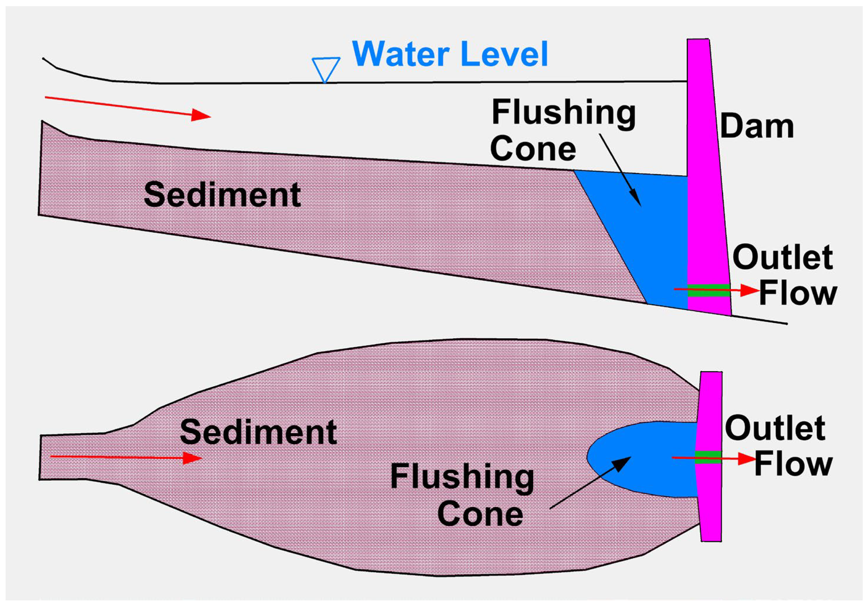
2.3. Pressure Flushing

Pressure flushing has been widely used for reservoirs where water storage is important and the inflowing sediment rate is relatively small. A key benefit of the pressure flushing is that much less water is released. Sediment removal, however, is usually limited to the vicinity of the outlets [30,31], as illustrated in Figure 2. Pressure flushing is often used to clean sediment and debris near water intake outlets. In general, the pressure flushing schedule adopted—the timing, duration, and release rate—may impact significantly the flushing process.

Our current practice of pressure flushing is mostly empirical. The flushing design is based mostly on empirical relations, as reviewed in [32]. Upstream of a gate in an unbounded reservoir, potential flow analytical solutions were derived by [33]. They proposed that the maximum velocity ($u_{max}$) upstream of the gap where the flow depth was much greater than the gap diameter ($D$) might be computed by:

$$\frac{u_{max}}{U_0}=1-{\left[1+0.25{\left(D/x\right)}^2\right]}^{-0.5}$$

In the near gap zone of x/D < 2, where $x$ is the distance along the centerline from the gap, $D$ is the gap diameter, and $U_0$ is the average velocity within the gap. The maximum velocity is proportional to $x^{-2}$ for $x/D$ greater than 2. The analysis demonstrated that the flow velocity decreased rapidly upstream of the gap and, therefore, the effect of the gap on erosion was limited to a relatively small area upstream of the gap.

Powell and Khan [34,35] studied the flow field upstream of a bounded gap with both fixed and mobile beds. They analyzed a circular gap and the flow field was found to be similar to the unbounded gap. A similar generalized equation was derived as:

$$\frac{u_{max}}{U_0}=1-{\left[1+a{\left(D/x\right)}^b\right]}^{-c}$$

The $a$, $b$, and $c$ values were found to be 0.332, 1.679, and 0.515 for the fixed bed, and 0.145, 1.493, and 0.913 for the mobile bed.

A conceptual sketch of the scour cone upstream of a gap is shown in Figure 5. The scoured area is assumed to form at depth $D_s$ below the gap invert. There is a flat area projecting from the wall and then the scoured cone projects upstream at a constant angle $\theta$.

Fathi-Moghadam et al. [36] performed a series of physical modelling studies on non-cohesive sediment scouring under pressure flushing upstream of circular gaps. The equations developed were based upon laboratory data and did not incorporate field data. It is difficult to scale both the geotechnical processes and the fluid processes simultaneously, and laboratory relationships are not generally applicable to field situations.

More empirical equations have been developed by, e.g., [34,35,37,38,39]. Refer also to [32] for a more detailed review. It is sufficient to comment that the empirical equations are useful in designing and evaluating expected scour in pressure flushing, but the following limitations need to be taken into consideration:

• The empirical equations may not apply outside of the range of parameters used in their development.
• They do not describe all the characteristics of the scour hole.
• They apply only for simple geometric conditions. Other structures added may alter the scour significantly.
• The sediment size and cohesive properties were not scaled from the field to the laboratory. The non-dimensional parameters related to the sediment size may be quite different in the laboratory and in the field.

2.4. Turbidity Current Venting

Turbidity current may be formed if the incoming sediment is fine but the concentration is high. This is the result of sediment-laden flow plunging beneath clear water in the reservoir. Once plunged, the turbidity current usually moves along the reservoir bed towards the dam as an undercurrent (Figure 3). Such a bottom-moving turbidity current may be vented out of reservoir if there are low-level outlets opened at the right time. While the turbidity current is being vented, the reservoir deposits on the bed may also be entrained and removed out of the reservoir. Venting can be an effective sediment management technique that has been studied extensively [11].

Empirical and analytical analyses have been carried out and much information is available for understanding the turbidity current characteristics such as the plunging criteria, mixing rate, and entrainment from the upper clear water layer. The need to analyze and predict the turbidity current has also prompted the development of empirical/analytical tools. Representative works were documented by [40,41]. A large amount of information contained in [40] was used to develop an empirical tool DCURL at USBR [42].

The plunging point is an important parameter that might be determined empirically. In a narrow reservoir, the plunging flow will form a line across the width. When a sediment-laden flow discharges into a wide reach, the turbid water may extend into the reservoir as an irregular tongue-like current which may shift from one side of the impoundment to the other. The location of the plunge point may be determined by the balance between the inflow momentum, the pressure gradient across the interface separating the river and reservoir waters, and the resisting force. The location is also influenced by morphological factors (bed slope, bed friction, and cross-sectional area). It can move several kilometers in a few hours in response to the dynamic flows due to a storm or the hydropower operation. For example, the water depth at the plunge point may be estimated using the densimetric Froude number at the plunging point as [5]:

$$F_p=\frac{V_i}{\sqrt{g^{\prime }{h}_p}}; g^{\prime }=\frac{{\rho }_i-{\rho }_a}{{\rho }_a}g$$

where $V_i$ is the depth-averaged velocity of the incoming flow, $h_p$ is the depth at the plunging point, and ${\rho }_a$ and ${\rho }_i$ are the densities of the ambient and the incoming waters, respectively. Both laboratory and field data showed that $F_p$ had a value of about 0.78, although other values were also reported [5]. Different values of $F_p$ were mostly associated with the different assumed cross-section geometries. See [43] for a summary of the various $F_p$ values.

Entrainment and mixing of the ambient clear water into the incoming turbid water occurred both in the plunging zone and after the turbidity undercurrent formed. The entrainment processes into the undercurrent are well suited to laboratory studies and have been carried out for simple cases such as [43,44]. Entrainment and mixing within the plunging zone have received less attention, although up to 80% of the total entrainment might occur in this zone [40]. Initial mixing at the plunging point is complex and empirical equations have been derived and discussed (e.g., [40,43,45]). Later, Fleenor [46] developed a new method to compute the initial entrainment, which varied from 30 to 300 percentage of the initial inflow. The study described the process of initial entrainment in the plunging zone, parameterized mixing, and developed and validated a computer tool that fully accounted for the initial mixing over a range of flows and conditions expected in natural water bodies.

Entrainment after the plunging zone has been analyzed extensively. One-dimensional density underflows are governed by equations similar to the backwater equations of an open channel flow. Detailed mathematical derivations and treatments are available in the literature such as [47]. Analytical solutions to the simplified equations are often used by the empirical/analytical tools. In such models, the entrainment rate for the underflow appeared in the volume conservation law, as follows [40]:

$$\frac{𝜕A}{𝜕t}+\frac{𝜕V_{b0}A}{𝜕x}=E{V}_{b0}B$$

where A is the cross-sectional area, B is the channel width, $V_{b0}$ is the revised velocity downstream of the plunging point, and E is the entrainment rate. A number of entrainment relations were developed and used. For example, Ashida and Egashira [48] used the following expression:

$$E=0.0015R_i^{-1}; R_i=\frac{{\rho }_i-{\rho }_a}{{\rho }_a}\frac{g{h}_{b0}}{V_{b0}^2}$$

where $h_{b0}$ is the water depth at the plunging point. See [49] for other alternatives.

$$E=0.5{\eta }^3{C}_k{C}_b^{1.5}{R}_i^{-1}$$

3. Literature Review: Numerical Models

Numerical models which solve the partial differential equations (PDE) of the basic conservation laws have been widely used in hydraulic flushing studies, as the empirical/analytical methods have limitations. The model complexity varies widely, ranging across 1D, 2D, and 3D. A literature review is provided below concerning these models, as a comprehensive review has not been carried out, although limited reviews are available [24,50].

3.1. One-Dimensional Numerical Models

One-dimensional numerical models require the computing resources and are thus widely used for long-term simulations. However, care needs to be taken as 1D models have their own limitations; for example, they are primarily for run-of-the-river or narrow reservoirs where flow is highly channelized and transverse mixing is well accomplished [50]. Previous 1D modeling studies are reviewed below.

Morris and Hu [51] used the 1D HEC-6 to simulate sediment flushing in the Loíza Reservoir in Puerto Rico. The numerical study indicated that the conversion of the reservoir from the continuous high-pool operation to the low-pool operation during flood periods had the potential to reduce the sediment trap efficiency by 65%.

Chang et al. [52] used a 1D FLUVIAL-12 model to evaluate the feasibility and effectiveness of drawdown flushing during a flood. A series of reservoirs were examined on the North Fork Feather River in Northern California. The numerical modeling demonstrated that that sediment could be flushed and the reservoir capacity could be maintained by adopting an extended drawdown flushing operation. It was further shown that the reservoir drawdown operation and reservoir operation could be controlled such that no sand would be deposited on the gravel bed downstream of the reservoirs for fish habitat benefits.

Liu et al. [53] reported a 1D numerical modeling to simulate the 2001 sediment flushing operation at two reservoirs in a series—the Dashidaira and Unazuki reservoirs on the Kurobe River in Japan. The model computed the bed evolution, suspended sediment concentration, and the sediment volume flushed from or deposited in the two reservoirs.

Ahn et al. [54] applied the 1D GSTAR4 to simulate sediment flushing in the Xiaolangdi Reservoir on the Yellow River, China, as well as in the Lewis and Clark Lake on the Missouri River, USA. Useful results were reported.

Guertault et al. [55] applied the 1D Mage-AdisTS to simulate the 2012 sediment flushing at the Genissiat Reservoir on the French Upper Rhone River. During the flushing, water and sediment were released at different levels to maintain the average downstream concentration below 5 g/L throughout the operation. Flushing outlets were located at three different levels and varied gate opening schedules were used to achieve the desired result. The model reproduced the sediment concentration at the three vertical outlets well.

Boyd and Gibson [56] used the 1D HEC-RAS model to simulate the 2014 flushing of the Spencer Dam reservoir, about 40 miles upstream of the confluence of the Niobrara River and the Missouri River. The reservoir has been flushed twice annually, spring and fall, for the last 60 years for sediment management. The numerical model was calibrated using the measured data. It was reported that the model underpredicted the delta scour by about 50% and over-predicted the peak downstream sediment concentration. The authors attributed the mismatch to the channel widening process that was not captured by the model. The same 1D model was also applied to the hydraulic flushing studies in other reservoirs, such as those reported in [57].

Brignoli [58] applied the SRH-1D model to simulate the controlled sediment flush at Isolato and Madesimo Reservoirs in Italy. The Madesimo Dam is on the Scalcoggia River, a tributary of Liro River, and about 1.4 km upstream of the confluence of Scalcoggia and Liro rivers. Isolato Dam is about 1.4 km upstream of the same confluence in the Liro River. The numerical model was used to predict the sediment impact downstream of the two dams and at the confluence. A satisfactory agreement between the computed and observed depositional patterns was obtained.

Huang et al. [11] updated the SRH-1D model to evaluate the sediment flushing operation at the Paonia Reservoir on the Muddy Creek, Colorado. A flushing plan was designed to lower the reservoir pool in early spring and flush the sediment during the spring runoff. Model modifications included the input of the user-defined reservoir operation rules. The model was first calibrated using 3 years of field data under the existing condition, and was then applied to predict the sediment management effects under different reservoir operation plans. The goal was to maximize the sediment flushing while maintaining the reservoir fill of water from the spring snowmelt. The timing of when sluicing was stopped and the storage of water was begun was based on the forecasted spring snow melt volume. The modeling showed that the reservoir trap efficiency depended strongly on the exceedance percentage of the inflow volume forecasted. For 2016, for example, the trap efficiency was 20% with the 90% exceedance, but 3% (net erosion) when the exceedance was 10%.

3.2. Two-Dimensional Numerical Models

Two-dimensional depth-averaged numerical models provide a more detailed representation of the reservoir hydraulic characteristics which might be missed in cross-sectionally averaged 1D models. Two-dimensional models are more general than the 1D ones in that they are applicable to both narrow and wide reservoirs and whether sediment deposition and resuspension vary or not across the channel.

Olsen [59] reported a 2D numerical model for sediment flush studies. The numerical model SSIIM solved the 2D depth-averaged equations for the flow and the 3D convection–diffusion equation for the sediment concentration. The mesh was made adaptive in the vertical direction and changed according to the water and bed levels. The numerical model was evaluated by comparing with the physical model data obtained for the Kali Gandaki Hydropower Reservoir in Nepal. Later, the 3D version of SSIIM was also reported [60].

Dewals et al. [61] used the WOLF 2D model to simulate sediment flush in an unknown reservoir in India. The 2D modeling was based on the multi-block rectangular mesh. The model predicted that only a narrow channel was generated by the flushing that was unable to be extended to the broad part of the reservoir width. The results demonstrated the ability of the model to simulate the sediment entrainment well during flushing; no measured data, however, were available to validate the numerical results.

Boeriu et al. [62] reported case studies using the 2D version of Delft3D for reservoir drawdown studies. Erosion was calculated differently for cohesive and non-cohesive beds, and the bed level was computed using the Exner equation. Case studies were reported in an unnamed reservoir in Sri Lanka where multiple days, 5 to 10, of drawdown flushing were simulated. Modeling was also performed at the Koga reservoir in Ethiopia with a 35-day drawdown. No measured field data, however, were available to validate the model results.

Chen and Tsai [63] developed a 2D model to simulate the sediment flushing efficiency of the A-Gong-Dian Reservoir in southern Taiwan. The reservoir was wide and the dam length was 2.4 km. The reservoir received waters from both Joushui River and Wanglai River. The flushing efficiency simulated by emptying the reservoir was found to match that based on the laboratory physical modeling study. The numerical modeling predicted the erosion upstream of the outlet on the Joushui river side and the deposition on the Wanglai river side. Based on the study, relocation of the outlet was proposed towards the Wanglai river side to improve the flushing efficiency.

Iqbal et al. [64] used the 2D BASEMENT model to simulate the sediment flushing processes. The model was based on the finite volume technique to solve the 2D shallow water equations on an unstructured triangular mesh. The transition from subcritical to supercritical during the rapid sediment flushing process was handled by solving the Riemann problem at cell interfaces using the Godunov scheme. The model was used to simulate two sediment flushing cases: a 1:40 physical model of the reservoir at the Gulpur Hydropower Plant on the Poonch river in the Pakistan-administrated Kashmir and the laboratory flushing experiment of [65]. The model was found to reproduce the bed longitudinal and lateral erosions as well as the flushed sediment volume.

Chaudhary et al. [66] used MIKE21C to simulate reservoir flushing at a proposed reservoir on the Dibang River in East Asia. The reservoir will collect water from the Dri and Tangon Rivers. The 1D MIKE 11 was used to calculate the long-term sediment distribution in the reservoir, while MIKE21C was used to simulate sediment flush under a proposed drawdown plan. Reservoir flushing was carried out through the low-level spillway and the downstream water surface was from the flow rates over the spillway. The numerical model estimated the amount of sediment that would be flushed out under various flushing schemes.

Stillwater Sciences [67] reported the use of the SRH-2D model to simulate the sediment processes under the dam removal scenarios at the Matilija Dam within the Ventura River watershed in southern California. One-dimensional sediment transport modeling was conducted first to determine the downstream project impact within the Matilija Creek and Ventura River. Later, it was determined that 2D modeling was needed to provide more detailed data in areas having potential flood risks.

SRH-2D has also been adopted to study several reservoir drawdown scenarios in the A-Gong-Dian Reservoir, Taiwan [68]. The study examined and then determined the main factors that would influence the flushing efficiency. Recommendations were developed on how to increase the sediment flushing efficiency. Modeling studies confirmed the benefits by lowering the initial water level, creating narrower gorge-like geometry by partitioning and modifying the operation rules related to the flushing duration and the release rate.

3.3. Two-Dimensional Turbidity Current Model

Turbidity current modeling is complex and empirical models have been widely adopted. Most existing numerical models cannot be used to simulate turbidity current transport in reservoirs once the sediment has plunged to the bottom. A few advanced models, however, have been reported to overcome the limitations of the empirical/analytical tools and the existing 2D models; they range across 2D laterally averaged models, 2D layer-averaged models, and 3D models.

The 2D laterally averaged model has been widely used for stratified flows in reservoirs, particularly in the field of water quality modeling. For reservoirs, when the variation in key variables over the depth is more important than the lateral changes, 2D equations may be derived by integrating the 3D equations laterally across the reservoir to obtain the so-called laterally averaged equations. Wells and Gordon [69] have shown that such models may be adequate for some reservoirs.

The limitations of the laterally averaged 2D models, however, are similar to the 1D models: they are suitable primarily for relatively narrow reservoirs where the water surface level does not vary appreciably and there are no significant lateral inflows or outflows. A key advantage of the 2D models over the 1D ones is that the vertical stratification may be simulated directly. Laterally averaged models may be classified as with or without hydrostatic assumption. A widely used 2D, laterally averaged, hydrostatic, hydrodynamic, and water quality model is the so-called CE-QUAL-W2 [70]. This model assumes that vertical velocities are sufficiently small so that the vertical momentum equation may be reduced to the hydrostatic condition. The model has been widely adopted to simulate narrow reservoirs such as [71,72].

For wide or general reservoirs, layer-averaged 2D models are more appropriate for the turbidity current modeling. A complete set of layer-averaged governing equations was reported in [47]. Only a handful of 2D layer-averaged models have been reported that can deal with unsteady and non-conservative turbidity currents. One of these was the work of Bradford and Katopodes [73], who studied turbidity undercurrents in the deep-sea environment. A high-resolution, total-variation-diminishing, finite-volume numerical model was developed to capture the current front using the predictor–corrector time-stepping scheme. Mesh was used to represent the geometry suitable to deep sea applications. The model was verified by comparison with the experimental data of turbidity currents driven by uniform and non-uniform sediment. Groenenberg et al. [74] reported a 2D model that used a combination of the explicit fractional-step MacCormack scheme and a high-resolution shock-capturing technique. The model was based on a rectangular mesh and used a second-order finite-difference approximation. The model was verified using multiple laboratory cases; reasonable agreements with the measured data were reported.

A general 2D layer-averaged turbidity current model was developed by Lai et al. [75], and applications were reported in [76]. An extensive number of verification cases was documented which highlighted the applicability range of the model. Later, a case study will be presented and discussed using the model. We believe that the 2D layer-averaged model is a good compromise between the empirical/analytical models that are over-simplified and the 3D models that are still at the research stage and yet to become practical.

3.4. Three-Dimensional Numerical Models

Three-dimensional numerical models have also been reported in simulating reservoir drawdown flushing. Some models are limited to hydrostatic assumption, for which an extensive review was presented in [77]. In the following, only the non-hydrostatic 3D models are reviewed. We will use the term “3D CFD (computational fluid dynamics) models” to refer to this model category. Note that the full Navier–Stokes (NS) equations are solved with such models along with an appropriate turbulence model. Our experience suggested that only a 3D CFD model would be beneficial in obtaining more accurate results than the 2D layer-averaged models, at least for hydraulic flushing modeling studies.

Ghoreishi and Tabatabai [78] reported the use of a 3D CFD model to simulate the reservoir sediment flushing experiment carried out by [65]. The experiment was conducted in a rectangular flume which had dimensions of 50.0 m long, 2.44 m wide, and 1.52 m high, and the sediment was paved in a 9 m reach upstream of the dam. The numerical model predicted the channel erosion near the dam well; however, it did not reproduce the observed channel erosion further upstream longitudinally. The authors attributed the mismatch to the assumption of the rigid lid for the water surface. Temporally, the 3D model reproduced the erosion patten in the initial stage of the flushing well and showed differences in the later stages. Results indicated that the model performed well for the pressure flushing process, but less good for the later drawdown processes.

Haun and Olsen [79] applied the 3D SSIIM to predict reservoir sediment flushing processes. The model used the structured mesh in the horizontal plane and adaptive grid in the vertical direction. Only one vertical cell was adopted in the shallow area, while up to eleven cells were used in the deep area. The model was applied to simulate a physical model case conducted at the Kali Gandaki hydropower reservoir in Nepal. Later, Olsen and Haun [80] updated SSIIM to include the bank failure module to improve the prediction of channel widening processes during reservoir flushing. The model domain was divided into water, soil, and slide cells. The soil domain used a 2D horizontal mesh, while the water and slide domains were based on a 3D mesh. The bank failure algorithm was tested for the 2014 reservoir flushing event at the Bodendorf reservoir, Austria. The model was able to reproduce the number and magnitude of the slides well, although the locations were not always correct. The updated model worked well for thick sediment layers, but instabilities occurred for thin layers. SSIIM was also used in [81] to simulate the flushing efficiency of the Schwarzenbach Reservoir in the Black Forest, Germany, under both the partial and full drawdowns.

Esmaeili et al. [82] employed the SSIIM model to simulate the 2012 sediment flushing operation at the Dashidaira Reservoir in Japan. The sediment flushing operation was performed at the site through the bottom outlets annually in the early rainy season from 1991. The model was first calibrated by reducing the difference between the computed and measured total flushed-out sediment volume. The simulated reservoir bathymetry after flushing was compared with the measured data. The results showed that the 3D model simulated reasonably well the flushing channel evolutionary pattern. Modeling found that finer sediment was entrained and flushed out earlier than the coarser sediment. They later presented additional modeling studies using the same model by adding additional artificial discharges during the free-flow state [83], increasing the drawdown speed, and adding an auxiliary longitudinal channel.

Our review found that numerical modeling of the pressure flushing processes is rarely carried out. It is possibly because only 3D CFD modeling is adequate for the pressure flushing simulation. An attempt was reported by Ermilov et al. [84], who used the TELEMAC-MASCARET package to simulate the pressure flushing scenarios. Model results were compared with the physical model data. It was shown that 3D modeling was capable of simulating sudden sediment removal in a schematized reservoir under the pressure flushing operation. The model reproduced the typical scour cone shape upstream of the flushing gate; locally varying flow features were also captured. The simulated bed scouring changes were in good agreement with the results of the physical model study. It was also found that the 3D model results were sensitive to the numerical model parameters adopted.

Three-dimensional CFD modeling was also carried out by Lai and Greimann [32] to simulate the pressure flushing process at the Cherry Creek Reservoir, Denver, Colorado. The numerical model results were compared with the field data and good results were obtained. Further discussion of the case will be presented later in this article.

3.5. Nested Approach

It has been commented that the so-called Nested Approach has been adopted for the numerical modeling of hydraulic flushing and can be beneficial. Often, a comprehensive reservoir management/sustainability study may adopt the nested approach in which 1D, 2D, and 3D models are applied conjunctively. In this approach, 3D modeling is applied in a subset zone of the 2D model, and 2D modeling is a subset of the 1D model domain. Often, the coarser models provide the boundary conditions to the refined ones. The nested approach has the best potential to address an extensive list of study questions and may be adopted for large projects.

Castillo et al. [85] provided an example of the nested approach to understand the changes expected in the Paute River, Ecuador, after the Paute-Cardenillo Dam was constructed. Then, 1D, 2D, and 3D models were used together to answer various study questions related to the sediment transport and flushing consequences. The 1D model was used to estimate the long-term reservoir sedimentation; the 2D model was used to simulate the 72 h hydraulic flushing operation; and the 3D model was applied to investigate the sediment transport details when the bottom outlets were operated. The study demonstrated that different model simulations were needed to achieve appropriate resolutions in the prediction of the sedimentation and flushing operation. The reported computing times of all models by Castillo et al. [85] may shed light on the model performance. The 2D modeling of a 72-h period took about 24 h in computing time for the entire reservoir, while 3D modeling of the same period required above 1600 h. The run time for the 1D model was not reported; we estimate that a 1D model would require only an hour to run a 100-year simulation.

4. Guidelines

In this section, general and specific guidelines are presented based on years of experience in research, development, and application at USBR.

4.1. General Guidelines

General recommendations are first presented on how to select a 1D, 2D depth-averaged, or a 3D CFD model.

For 1D models, a key advantage is that a minimal amount of computing time is required so that a long-term modeling study may be conveniently carried out. A list of general guidelines is provided below for using the 1D model:

• Recommended for projects whose study questions require long-term simulations (e.g., >10 years); a 100-year modeling study has been routinely carried out.
• More appropriate for evaluating alternative operational options or design strategies when many simulations are needed.
• Study questions that may be answered by 1D models include: reservoir sedimentation and storage loss, long-term flushing efficiency for different flushing alternatives, reservoir sustainability impacts of reservoir operation, long-term sediment impact downstream of the reservoir, and quantification of the uncertainty of the model results, among others.
• One-dimensional modeling can often start from the pre-impoundment geometry and use the historical inflows and reservoir operations as the inputs for the model calibration. Measured longitudinal profiles and/or the reservoir sedimentation volumes at different times may often be used for the model calibration.
• Limitations of 1D modeling should be kept in mind, such as:

  ∘

  High uncertainty exists when the reservoir is wide and geometry is not a single channel. However, 1D model accuracy improves significantly with a narrowing reservoir channel. A reservoir is considered narrow when the width ratio of the largest reservoir cross section to the narrowest or drawdown section is less than 4 to 5.

  ∘

  The reliability of the 1D results increases with the pool level lowering depth. The highest accuracy is achieved when the flow during the flushing is of the run-of-the-river type.

For 2D depth-averaged models, the computing time may be much longer than 1D models. Therefore, the spatial extent and simulation time duration may be limited. Specific guidelines/comments are as follows:

• Spatial and time limitations: the longitudinal length along the river is not higher than, e.g., 20 km, and the simulation time is often limited to a single drawdown event or no more than a few years.
• Two-dimensional modeling is generally applicable to most reservoirs, and particularly recommended if the reservoir width is large (more than 4 to 5 times of the drawdown width) or if the assumption of a constant water level across the cross sections is not valid. Tow-dimensional modeling is highly recommended if the delta evolution will be simulated where the delta moves into lateral tributaries and margins.
• Two-dimensional modeling is needed where multiple gates are used for drawdown across the dam and when gates are operated differently.
• Potential limitations:

  ∘

  The flushing-induced channel erosion may be underpredicted significantly if the bed consists of cohesive materials, unless the cohesive properties are properly taken into consideration and the model is properly calibrated.

  ∘

  Channel erosion during drawdown may be under-predicted significantly if the erosion is mainly contributed by bank erosion or knickpoint process.

Three-dimensional CFD models refer to those which solve the Reynolds-Averaged Navier–Stokes (RANS) equations without the use of the hydrostatic assumption. General guidelines are provided below:

• Three-dimensional models are the most general and applicable to all types of hydraulic flushing.

  ∘

  In contrast, 1D and 2D models have restrictions due to the various model assumptions adopted. For example, 1D and 2D models are generally not applicable to pressure flushing, as velocity is assumed to be uniform throughout the pool depth with such models. For pressure flushing, 3D modeling is probably the only viable option.

• Few adjustable model parameters are needed for 3D CFD models, so model calibration is not critical, at least for the flow field processes. Please refer to [86] for a recent review of the 3D CFD models on sediment modeling. Three-dimensional CFD models, therefore, are highly recommended if the flow field, particularly in the vertical direction, is important to answer the study questions.

  ∘

  Model input parameters that may impact the model accuracy include mesh size, time step, and turbulence model.

• It is cautioned that most existing 3D CFD models adopted similar sediment theory and equations to the 2D depth-averaged models [75].

  ∘

  Therefore, any model errors associated with the sediment theory/equations would not be improved by using the 3D models.

• An important 3D model limitation: the runtime can be very high and days or even weeks have been reported in case studies. Therefore, both the spatial extent and time duration may need to be much reduced from the 2D models.
• Other general guidelines:

  ∘

  Model results may be sensitive to the mesh resolution; in general, a mesh sensitivity study should be carried out.

  ∘

  The selection of a turbulence model may not be critical in applications (though it has been reported to be significant in the literature, but mostly for theoretical studies), and may be treated as a secondary issue.

  ∘

  The accuracy of the scour and sediment predictions is additionally dictated by the empirical sediment equations adopted by the 3D model; therefore, sediment input parameters need to be carefully selected.

  ∘

  The bed sediment in front of the bottom gates is often cohesive for reservoir management applications; care should be taken to ensure that the model has cohesive bed modeling capability and that the cohesive erosion properties are adequately measured with known uncertainty ranges. Proper model parameter sensitivity studies may be important in obtaining statistically meaningful results.

4.2. Specific Guidelines

4.2.1. Drawdown Flushing Modeling

• One-dimensional or two-dimensional models are recommended for drawdown flushing simulation unless the pool water level is too high and the sediment processes are similar to pressure flushing.
• The reservoir narrowness should be used as a guide for the choice of 1D or 2D models (discussed previously). In theory, there is no width restriction with the 2D models.
• The reliability of 1D and 2D model results near the dam is influenced significantly by the amount of pool level lowering—the lower the pool level, higher the accuracy.
• Three-dimensional modeling may still be needed for the early stage of the drawdown flushing operation.

Two channel erosion processes should be recognized during drawdown: progressive and retrogressive. Progressive erosion is characterized by the emergence of an eroded channel at the upstream of the reservoir, and erosion moves downstream towards the dam and finally reaches the dam while the reservoir is being emptied. Channel formation is via fluvial processes of increased sediment-carrying capacity. Progressive erosion is often initiated when reservoir drawdown is achieved through low-level outlets and the drawdown rate is not rapid. This type is relatively easier to simulate than the retrogressive one. Retrogressive erosion is characterized by a zone of high slope and fast erosion that is moving upstream. The point of slope change has the highest erosion rate (commonly called the knickpoint). Retrogressive erosion may initiate in instances where sediment deposits are deep and near the dam and drawdown rate is rapid or an initial steep slope is created. This erosion type has been observed both in the laboratory and in the field [5]. Retrogressive erosion is much more difficult to simulate as knickpoint erosion may not be incorporated in most numerical models.

4.2.2. Turbidity Current Venting Modeling

• Empirical/analytical models may be used first at the beginning of a project to gain an overview of the turbidity current processes and obtain an estimate of general parameters such as the plunging point location and mixing characteristics. Not all turbid water would plunge to the reservoir bottom and form an undercurrent. Field observations and data may also be needed to gain an understanding of the turbidity current characteristics.
• Two-dimensional layer-averaged models are recommended for most projects as recent two-dimensional models are more general than the existing one-dimensional models and the computing time is becoming reasonable with the availability of fast modern-day PCs. In particular, turbidity current modeling is often event-based, so the simulation time is finite. If 1D models are used, ensure that the river resembles the run-of-the-river type.
• Three-dimensional CFD models may also be used and they are accurate. However, the runtime of most 3D models may be prohibitively long; 3D models are yet to become practical.

4.2.3. Pressure Flushing Modeling

• Only 3D CFD models may be appropriate for pressure flushing simulation. One-dimensional and two-dimensional models are not recommended unless the specific case study questions warrant their use.
• Only a portion of the reservoir pool near the pressure flushing bottom outlets needs to be simulated. Use of the entire reservoir is generally unnecessary and serves only to increase the computing runtime. The reason is that the scour cone is usually small and limited to the front part of the outlets. Away from the outlets, flow velocity is low and there is little sediment movement.

5. Case Studies

Case studies are provided in this section to shed light on the use and performance of the numerical models, as well as the use of the guidelines.

5.1. One-Dimensional Modeling at Paonia Reservoir, Colorado

SRH-1D model has been applied to several drawdown sediment flushing studies at USBR. Herein, the modeling at the Paonia reservoir, Colorado, was chosen to illustrate the selection, use, and performance of 1D modeling.

The Paonia Reservoir on the Muddy Creek is located about 27 km northeast of Paonia, Colorado. The reservoir has a surface area of 1.35 km², a total design capacity of 25.8 million-m³, and is considered narrow (4.8 km long and 0.3 km wide). Hydrology is characterized by spring snowmelt with summer thunderstorms. The estimated average annual sedimentation rate is about 0.125 million m³ per year; nearly 25% of the reservoir capacity has been lost. In 2010, the outlets were blocked by sediment and debris, leading to the start of a comprehensive study to design a sediment flushing plan to solve the sedimentation problem. Field drawdown flushing was exercised and able to pass sediment through the reservoir. However, it was insufficient to sustain the reservoir storage. In 2014, the dead pool of the reservoir was completely filled (Figure 6).

A numerical modeling study was initiated, using the SRH-1D model, to evaluate both the short-term and long-term plans [10,11]. Modeling provided answers about the reservoir sedimentation rate, trap efficiency, sediment release concentration, and other variables. One-dimensional modeling was adequate for the case, as the reservoir is relatively narrow and it was chosen as the study questions were related to the long-term effect of the flushing alternatives. The set of user-definable reservoir operation rules include (a) the minimum and maximum reservoir releases at different reservoir water levels, (b) timing to start reservoir filling according to the forecast incoming flows, (c) constraints on the releases imposed by the gate and spillway capacity, and (d) constrains on the ramping rate of the releases.

The model inputs included cross-sectional geometry, incoming flow and sediment rates, downstream water surface elevation or discharge, bed sediment size and gradation, flow roughness coefficient, sediment transport capacity equation, and other model-specific inputs. The model was first calibrated using the data collected in the time period of 11 June 2013 to 30 June 2015. The measured sediment load at the reservoir exit was used for the model calibration. It was found that the reservoir channel bed profile and the outflowing suspended concentration were predicted reasonably by the model. The calibrated model was then used for both the short-term and long-term simulations for model application predictions. The impact of various reservoir operational rules was evaluated.

5.2. Two-Dimensional Depth-Averaged Modeling of Drawdown Flushing on the Klamath River, Oregon

Two-dimensional modeling has been routinely carried out at USBR for numerous sediment transport projects. Herein, the study of the drawdown processes at the Copco-1 Reservoir on the Klamath River, Oregon is presented—a 2D modeling study of hydraulic drawdown flushing. The study was carried out as part of a much larger effort at USBR to support the Secretarial Determination on Klamath Dam Removal and Basin Restoration [87].

Four dams, JC Boyle, Copco-1, Copco-2, and Iron Gate on the Klamath River, were studied for possible decommissioning. Numerical modeling was carried out at the Copco-1 Reservoir to address two study questions: (a) channel erosion during drawdown, and (b) the estimate of suspended sediment concentration released to the downstream. The drawdown process was event-based (a relatively short time period) and the reservoir was relatively wide (erosion was expected to have lateral variation)—these two facts led to the selection of 2D modeling for answering the study questions. The modeling study was further used to aid in determining the strategies for revegetating the reservoir area and recovering a functional riparian corridor after dam decommissioning. The downstream sediment release would help to determine the proper timing, duration, and release rate of the drawdown design. Note that extensive 1D modeling was also carried out to answer other long-term questions, as documented in [87].

Copco-1 Dam, constructed in 1918, is 38.4 m high; the reservoir is 7.5 km long, and has 10.4 m average depth and 41.6 million-m³ storage capacity. The 2D modeling began with the selection of a model domain (entire reservoir selected) and the generation of a 2D mesh (10,504 mixed quadrilaterals and triangles)—they are shown Figure 7a. Measured bathymetric and terrain data were used as the initial reservoir terrain before the drawdown (Figure 7b). Main model inputs included (a) the Manning’s roughness coefficient of 0.03; (b) bed and subsurface layer sediment data (the top layer consisted of mostly silt and clay and the bottom layers of coarse gravel); and (c) the historical upstream flow rate and zero sediment rate (as the majority was wash load that simply passed through).

Initially, the reservoir was filled with water to an elevation of 793.4 m (inversion of the spillway). Drawdown was then initiated through water release at the low-level gates. The release rate was 0.914 m/day but varied according to the gate constraint. The modeling used seven sediment size classes, with one size representing the cohesive material smaller than 0.0625 mm in diameter. Three simulations were carried out, corresponding to three hydrological scenarios (Dry-Year, Average-Year, and Wet-Year). Each run started on 15 November and ended on 15 May of the following year, a duration of six months.

In the following, the model results corresponding to the Average-Year, named the baseline, are presented. The predicted reservoir water surface elevation and discharges into and out of the reservoir are displayed in Figure 8. It can be seen that the reservoir elevation was lowered to below 762 m within one month. However, only under the relatively dry year could the reservoir water level be maintained at such a low level. The reservoir would be filled with water quickly with the Wet-Year hydrology. The predicted sediment concentration released to the downstream from Copco-1 is shown in Figure 9 for the three hydrological scenarios. The predicted concentration did not differ substantially between the Dry-Year and Average-Year, as both flows were sufficient to mobilize the majority of the reservoir deposits. There was, however, a noticeable difference between the Wet-Year and the other two. This might be explained by the fact that the reservoir water level remained low for the Dry- and Medium-Year but not so for the Wet-Year. Low water elevation led to high flow velocity and sediment carrying capacity. With the Dry- and Medium-Year simulations, the predicted sediment concentration pulse had an average peak of about 6000 ppm (occasionally exceeding 7000 ppm) and a duration of about 1.5 months. With the Wet-Year, the average pulse peak was lowered to 4000 ppm (occasionally exceeding 6000 ppm). After 45 days of the drawdown, sediment concentration fell to a low level (about a few hundred ppm).

One of the study questions involved understanding erosion channel formation due to the drawdown. As discussed earlier, two channel erosion forms may occur: retrogressive and progressive. The numerical modeling of Copco-1 showed that the channel process belonged to the progressive type, as shown in Figure 10. Progressive erosion was expected to occur, given the assumed drawdown conditions according to the analyses in [88,89]. The reservoir pool level was near its lowest on 29 December, while 14 May was the end of the simulation. The pre-dam geomorphology of the reservoir area was delineated in [87] and is plotted in Figure 11. The predicted bed elevation and the net eroded depth are compared with the initial top bed layer thickness and bed elevation in Figure 12. It is seen that the model-predicted channel erosion pattern and thalweg agreed well with the pre-dam channel. The majority of the reservoir deposits within the pre-dam channel had eroded after 45 days of the drawdown, particularly for the upstream half of the reservoir (note that the results are inaccurate near the dam). Incision into the bottom bed layer was also predicted for the upstream half of the reservoir six months after the drawdown. In the upstream zone 1 and 2 areas, channel incision decreased with increasing flow into the reservoir (wet year). The trend, however, was reversed in zones 4 and 5, where incision increased with an increasing flow.

Deposition was predicted in the pre-dam floodplain area in the downstream half of the reservoir. It was particularly visible in the open area near the narrow canyon. These model results provided the data needed to make the decision on how revegetation and habitat restoration would be planned after dam decommissioning.

It has been commented that the deposition near the drawdown gate in zone 1 may be unrealistic given that (a) the model was depth-averaged but flow was highly 3D near the gate, and (b) the pressurized flow dominated near the gate. The inaccuracy of the erosion prediction near the gate, however, was expected to have negligible effect on the predicted erosion upstream.

5.3. Two-Dimensional Layer-Averaged Modeling of Turbidity Current at Shihmen Reservoir, Taiwan

A 2D model of turbidity current venting at Shihmen Reservoir, Taiwan, is presented to highlight the modeling process and model performance. Suspended sediment periodically moves into this reservoir in the form of a turbid undercurrent during large typhoons. Limited sediment venting capacity at the dam has led to the loss of reservoir capacity at a faster rate than the original design. The 2004 Typhoon Aere event is presented here as a case study, as the event was large and caused 11% loss of the reservoir storage capacity.

The 2D turbidity current model of [75] was used for the modeling and the results were compared with the 1-to-100 scale laboratory data. The numerical model covered the entire reservoir with about 15.5 km longitudinal length (Figure 13a), and a 2D mesh was developed consisting of 33,008 mesh cells. Initial reservoir bathymetry was derived from the measured data surveyed in 2003 (Figure 13b). At the reservoir inflow boundary, measured flow rate and suspended concentration were used as the boundary conditions. The median diameter of the turbidity current sediment was 5 μm. The simulation was carried out for the typhoon period of 02:00, 24 August to 21:00, 26 August 2004—a 67 h duration in the prototype.

Downstream boundary conditions were complex and demonstrated the need for 2D modeling. There were five outlets distributed along the dam and located at different depths. They included the spillway, the flood diversion tunnel, the powerhouse intake, the permanent river outlet, and the Shihmen intake. The spillway had an invert of 235 m, width of 107 m, and discharge capacity of 5800 m³/s at the prototype scale. The flood diversion tunnel had an invert of 220 m, height of 8 m and a full-capacity discharge of 1800 m³/s. The powerhouse outlet vented the highest amount of sediment, as it was located at the lowest depth. It had an invert of 171 m, a height of 5 m and a full-capacity discharge of 380 m³/s. The permanent channel outlet was relatively small and less important in sediment venting. It had the same invert as the powerhouse but a full capacity of 30 m³/s. The Shihmen intake was also small in its venting capacity; it had an invert of 193.6 m, height of 2.4 m, and full capacity of 13 m³/s. The key model input was the drag coefficient; a value of 0.055 was adopted (calibrated). The initial reservoir was assumed to be clear (i.e., zero suspended sediment concentration without the undercurrent); the turbidity current then entered the model domain and moved towards the dam.

The predicted arrival times of the turbidity current at various cross-sections along the reservoir are compared with the measured data in Figure 14. Good agreement was obtained. The percentage error was less than 14% at all measured cross-sections. The numerical model predicted that it would take 0.925 h for the front of the current to reach the powerhouse from the upstream boundary (9.25 h in the prototype), which was comparable to 0.930 h of the physical model. The turbidity current front was predicted to move at a nearly constant speed of 0.0450 m/s; it was compared with the measured speed of 0.0448 m/s (0.448 m/s in the prototype). The results showed that the numerical model was capable of predicting the current movement through the reservoir well. Such predictions were important as they could help inform how the outlets might be operated to optimize the sediment venting.

Of particular interest was the total amount of sediment that might be vented out of the available outlets; this would produce the venting efficiency important for determining the reservoir storage loss and its sustained life. The sediment volumes delivered into and vented out of the reservoir through all outlets are compared in

Table 1. Summary of total sediment volumes moved into and out of the reservoir during the Typhoon Aere event from both the numerical and physical models.

	Numerical Model	Physical Model
Total sediment volume into reservoir (million-m3)	10.93	10.97
Volume through Power House (million-m3)	3.31 (30.3%)	3.18 (29.0%)
Volume through Spillway (million-m3)	1.72 (15.7%)	1.02 (9.30%)
Volume through Flood Diversion (million-m3)	0.754 (6.9%)	0.420 (3.92%)
Volume through Permanent Channel (million-m3)	0.265 (2.42%)	0.259 (2.36%)
Volume through Shihmen Intake (million-m3)	0.0569 (0.52%)	0.0593 (0.54%)

between the numerical and physical models. It was shown that the total sediment volume vented out of the reservoir was 55.9% and 45.1%, respectively, for the numerical model and physical model. The higher venting efficiency predicted by the numerical model was due primarily to the higher predicted sediment through the spillway and the diversion tunnel—the two higher-level outlets whose venting ability depended heavily on the vertical distribution of the turbidity current, which was not predicted by the 2D model and obtained through an empirical relation.

A sensitivity study was also carried out with several model input parameters. It was found that the drag coefficient and erosional rate were important, while the entrainment rate was not. The drag coefficient impacted the current front speed significantly but had negligible effect on the outlet sediment rates. For example, the times needed for the current front to reach the powerhouse outlet were 8.20, 9.25, and 10.03 h, respectively, with drag coefficients of 0.035, 0.055, and 0.075. The erosional rate coefficient was important for predicting the erosion and deposition characteristics during the venting event as well as the current movement speed. An increased erosional rate coefficient led to increased sediment volume out of the reservoir and faster current movement speed.

5.4. Three-Dimensional CFD Modeling of Pressure Flushing at Cherry Creek Reservoir, Colorado

A 3D CFD modeling study is presented for pressure flushing at the Cherry Creek Reservoir, Denver, Colorado. Three-dimensional modeling is often required for pressure flushing, as the above guidelines recommended.

A small horizontal domain near the outlets was chosen for the 3D modeling according to the guidelines discussed above and shown in Figure 15a. The far field flows, indeed, were found to be small and insignificant for the present modeling, based on the results of an entire reservoir simulation (results not shown here). The flushing outlets were located within an intake tower whose dimensions are marked in Figure 15b and Figure 16. The outlet gate geometry needed to be represented as accurately as possible for adequate 3D modeling (see Figure 16). As can be seen, the five bottom gates were used for pressure flushing; they were extended out in the numerical model so that water release amounts might be implemented properly by the numerical model. The 3D mesh had a horizontal size of 9855 mixed quadrilateral and triangle cells (Figure 15a) and 47 vertical points. Note that the 3D model used solved the NS equations, and the k-ε turbulence model was adopted.

Two sets of modeling were carried out, corresponding to two pressure flushing operations at the Cheery Creek Reservoir: 2017 low-discharge and 2018 high-discharge flushing. The flushing release rate was an input in the model as the boundary condition, while other model inputs (to be discussed below) were kept the same for all modeling runs. Only the 2018 flushing results are discussed below.

Pressure flushing was conducted in the field on 23 May 2018 with a nominal discharge of 36.8 m³/s and the reservoir pool maintained at the constant elevation of 45.71 m. The actual flow release rate through all intake gates is shown in Figure 17. The release was achieved by opening one gate at a time of the five gates, and following the sequence of gates 3, 1, 2, 4, and 5 (gates are numbered from right to left looking towards the intake in Figure 16). The reservoir sediment consisted of clay, silt, and sand and the properties were measured by [90] and used by the model. The fractions for the clay, silt, and sand were 45%, 50%, and 5%, respectively. The bed was treated as cohesive. The erodibility properties of the cohesive sediment are important for modeling. The critical shear stress and erodibility were measured by [90]: the critical shear stress was 0.62 Pa and the erodibility was $3.55\times {10}^{-4}$ m/s-Pa.

First, the predicted sediment concentration out of the reservoir was compared with the field data in Figure 18. The agreement was found to be good, although the concentration was under-predicted over the first two gate opening periods and over-predicted in the next three gate periods. Note that the predicted concentration was obtained right after the gates (within the outlet works), while the measured value was within the Cherry Creek, about 0.4 km downstream of the dam outlet. This may explain some of the above discrepancies. The measured high concentration during the first gate was partially contributed by the sediments stored downstream of the release outlet, and not entirely due to the reservoir release.

The predicted erosion pattern (scour zone) produced by the pressure flushing is shown in Figure 19. The results showed that the scour zone was limited to within the intake, which was confirmed by the field survey at the site. A quantitative comparison of the erosion pattern was not possible as the field measurement was not able to reach inside the intake.

This case study shows that the 3D CFD model performed well in simulating the pressure flushing process, at least for the study site. For example, the sediment concentration released downstream was well predicted, pointing to its potential to be used for future pressure flushing modeling applications. It showed also that 3D numerical models may be useful in developing an effective flushing strategy. Based on the above results, for example, a three-gate release—gates 3, 1, and 5—would be more efficient than the current five-gate schedule. Further, the flushing efficiency might be maximized by flushing every other year or the flushing duration may be much reduced to save water release, as high erosion occurs primarily during the early stage of gate opening.

6. Concluding Remarks

A comprehensive review has been provided in this article with regard to the numerical modeling of hydraulic flushing to manage reservoir sedimentation. Three sediment removal types were covered: drawdown flushing, pressure flushing, and turbidity current venting. The review also provides the empirical/analytical methods that may be used for a quick assessment of the three types of hydraulic flushing, while the more comprehensive and general 1D, 2D, and 3D models were reviewed extensively. In particular, guidelines and best practices were presented for the three categories of the numerical models: 1D cross-sectionally averaged, 2D depth-averaged or layer-averaged, and 3D CFD models. Case studies were presented for each hydraulic flushing type and using each category of the numerical models. These cases illustrate the guidelines and discuss how study questions may be addressed. In addition, the case studies also discuss how a model is selected given a specific reservoir, the determination of the model domain and mesh, model inputs, model performance, and a results comparison. Important findings include the following: (a) the empirical/analytical method may be used for planning studies; (b) 1D, 2D, and 2D models are recommended for design and alternatives assessment studies; (c) 1D models are appropriate for narrow reservoirs or long-term simulations; (d) 2D models are recommended for wide reservoirs or where later changes are important; (e) 3D models are needed for pressure flushing modeling or any near-field processes for which vertical variation is important (1D and 2D models are not adequate); and (f) any numerical models need to be calibrated and/or validated for the study site before the results may be used for predictions.

References

- Annandale, G.W.; Morris, G.; Karki, P. Extending the life of reservoirs: Sustainable sediment management for dams and run-of-river hydropower. In Directions in Development; World Bank Group: Washington, DC, USA, 2016. [Google Scholar]
- Moriasi, D.N.; Steiner, J.L.; Duke, S.E.; Starks, P.J.; Verser, A.J. Reservoir sedimentation rates in the Little Washita River experimental watershed, Oklahoma: Measurement and controlling factors. J. Am. Water Resour. Assoc. 2018, 54, 1011–1023. [Google Scholar] [CrossRef]
- Shelley, J.; Kenney, M.; Layzell, A.; Brown, T. Contribution of Two Eroding Banks to Multipurpose Pool Sedimentation at a Midwestern Reservoir; Rep. No. ERDC/TN RSM-20-6; US Army Engineer Research and Development Center: Vicksburg, MS, USA, 2020.
- Shelley, J.; Boywer, M.; Granet, J.; Williams, A. Environmental Benefits of Restoring Sediment Continuity to the Kansas River; Rep. No. ERDC/CHL CHETN-XIV-50; US Army Engineer Research and Development Center: Vicksburg, MS, USA, 2016.
- Morris, G.L.; Fan, J. Reservoir Sedimentation Handbook: Design and Management of Dams, Reservoirs, and Watersheds for Sustainable Use; McGraw Hill Professional: New York, NY, USA, 1998. [Google Scholar]
- Annandale, G.W. Reservoir conservation and sediment management. In Water Week; Water Bank Group: Washington, DC, USA, 2001. [Google Scholar]
- White, R. Evacuation of Sediments from Reservoirs; Thomas Telford: London, UK, 2001. [Google Scholar]
- Basson, G.R. Management of siltation in existing and new reservoirs. General Report. In Proceedings of the 23rd Congress of the International Commission on Large Dams, Brasilia, Brazil, 25–29 May 2009. [Google Scholar]
- Wisser, D.; Frolking, S.; Hagen, S.; Bierkens, M.F.P. Beyond peak reservoir storage? A global estimate of declining water storage capacity in large reservoirs. Water Resour. Res. 2013, 49, 5732–5739. [Google Scholar] [CrossRef]
- Huang, J.; Greimann, B.; Kimbrel, S. Numerical Modeling and Analysis of Sediment Transport at Paonia Reservoir: SRH-1D Model Update, Calibration, Short-Term Prediction, and Long-Term Prediction; Report No. SRH-2016-30; Sedimentation and River Hydraulics Group, Technical Service Center, U.S. Bureau of Reclamation: Denver, CO, USA, 2016.
- Huang, J.; Greimann, B.; Kimbrel, S. Simulation of Sediment Flushing in Paonia Reservoir of Colorado. J. Hydraul. Eng. 2019, 145, 06019015. [Google Scholar] [CrossRef]
- Shelley, J.; Hotchkiss, R.H.; Boyd, P.; Gibson, S. Discharging Sediment Downstream: Case Studies in Cost Effective, Environmentally Acceptable Reservoir Sediment Management in the United States. J. Water Resour. Plann. Manag. 2022, 148, 05021028. [Google Scholar] [CrossRef]
- Shen, H.W. Flushing sediment through reservoirs. J. Hydraul. Res. 2010, 37, 743–757. [Google Scholar] [CrossRef]
- Randle, T.J.; Bountry, J.A.; Ritchie, A.; Wille, K. Large-scale dam removal on the Elwha River, Washington, USA: Erosion of reservoir sediment. Geomorphology 2015, 246, 709–728. [Google Scholar] [CrossRef]
- Madadi, M.R.; Rahimpour, M.; Qaderi, K. Improving the Pressurized Flushing Efficiency in Reservoirs: An Experimental Study. Water Resour. Manag. 2017, 31, 4633–4647. [Google Scholar] [CrossRef]
- Atkinson, E. The Feasibility of Flushing Sediment from Reservoirs; Rep. No. OD137; HR Wallingford: Wallingford, UK, 1996. [Google Scholar]
- Chaudhry, M.A. Worldwide experience of sediment flushing through reservoirs. Mehran Univ. Res. J. Eng. Technol. 2012, 31, 395–408. [Google Scholar]
- Batalla, R.J.; Vericat, D. Hydrological and sediment transport dynamics of flushing flows: Implications for management in large Mediterranean rivers. River Res. Appl. 2009, 25, 297–314. [Google Scholar] [CrossRef]
- Kantoush, S.A.; Sumi, T.; Suzuki, T.; Murasaki, M. Impacts of sediment flushing on channel evolution and morphological processes: Case study of the Kurobe River, Japan. In River Flow, Proceedings of the 5th River Flow Conference, Braunschweig, Germany, 8–10 June 2010; Dittrich, A., Koll, K., Aberle, J., Geisenhainer, P., Eds.; Bundesanstalt für Wasserbau: Karlsruhe, Germany, 2020; pp. 1165–1173. [Google Scholar]
- Antoine, G.; Camenen, B.; Jodeau, M.; Nemery, J.; Esteves, M. Downstream erosion and deposition dynamics of fine suspended sediments due to dam flushing. J. Hydrol. 2020, 585, 124763. [Google Scholar] [CrossRef]
- Sumi, T. Evaluation of Efficiency of Reservoir Sediment Flushing in Kurobe River. In Proceedings of the 4th International Conference on Scour and Erosion (ICSE-4), Tokyo, Japan, 5–7 November 2008; pp. 608–613. [Google Scholar]
- Kondolf, G.M.; Gao, Y.; Annandale, G.W.; Morris, G.L.; Jiang, E.; Zhang, J.; Cao, Y.; Carling, P.; Fu, K.; Guo, Q. Sustainable sediment management in reservoirs and regulated rivers: Experiences from five continents. Earth’s Future 2014, 2, 256–280. [Google Scholar] [CrossRef]
- Dahl, T.A.; Ramos-Villanueva, M. Overview of Historical Reservoir Flushing Events and Screening Guidance; Coastal and Hydraulics Laboratory, U.S. Army Engineer Waterways Experiment Station: Vicksburg, MS, USA, 2019.
- Anari, R.; Hotchkiss, R.H.; Langendoen, E.J. Elements for the Successful Computer Simulation of Sediment Management Strategies for Reservoirs. Water 2020, 12, 714. [Google Scholar] [CrossRef]
- Lai, J.S.; Shen, H.W. Flushing sediment through reservoirs. J. Hydraul. Res. 1996, 34, 237–255. [Google Scholar] [CrossRef]
- Shahmirzadi, M.M.; Dehghani, A.A.; Meftahh, M.; Mosaedi, A. Experimental investigation of pressure flushing technique in reservoir storages. Water Geosci. 2010, 1, 132–137. [Google Scholar]
- Chamoun, S.; De Cesare, G.; Schleiss, A.J. Managing reservoir sedimentation by venting turbidity currents: A review. Int. J. Sediment Res. 2016, 31, 195–204. [Google Scholar] [CrossRef]
- Annandale, G.W. Developments in Water Science-Reservoir Sedimentation; BV Rand Afrikaans University: Johannesburg, South Africa; Elsevier Science Publishers: Amsterdam, The Netherlands, 1987. [Google Scholar]
- Ackers, P.; Thompson, G. Reservoir sedimentation and influence of flushing. In Sediment Transport in Gravel-Bed Rivers; John Wiley and Sons: New York, NY, USA, 1987. [Google Scholar]
- Fan, J.; Morris, G.L. Reservoir sedimentation. II: Reservoir desiltation and long-term storage capacity. J. Hydraul. Eng. 1992, 118, 370–384. [Google Scholar] [CrossRef]
- Kantoush, S.A. Experimental Study on the Influence of the Geometry of Shallow Reservoirs on Flow Patterns and Sedimentation by Suspended Sediments. Ph.D. Thesis, EPFL, Lausanne, Switzerland, 2008. [Google Scholar]
- Lai, Y.G.; Greimann, B.P. Modeling of Cherry Creek Reservoir Pressure Flush; Report No. ENV-2020-83; Technical Service Center, U.S. Bureau of Reclamation: Denver, CO, USA, 2020.
- Shammaa, Y.; Zhu, D.Z.; Rajaratnam, N. Flow upstream of orifices and sluice gates. J. Hydraul. Eng. 2005, 131, 127–133. [Google Scholar] [CrossRef]
- Powell, D.N.; Khan, A. Scour upstream of a circular orifice under constant head. J. Hydraul. Res. 2012, 50, 28–34. [Google Scholar] [CrossRef]
- Powell, D.N.; Khan, A. Flow field upstream of an orifice under fixed bed and equilibrium scour conditions. J. Hydraul. Eng. 2015, 141, 04014076. [Google Scholar] [CrossRef]
- Fathi-Moghadam, M.; Emamgholizadeh, S.; Bina, M.; Ghomeshi, M. Physical modelling of pressure flushing for desilting of non-cohesive sediment. J. Hydraul. Res. 2010, 48, 509–514. [Google Scholar] [CrossRef]
- Kamble, S.A.; Kunjeer, P.S.; Sureshkumar, B.; Isaac, N. Hydraulic model studies for estimating scour cone development during pressure flushing of reservoirs. ISH J. Hydraul. Eng. 2017, 24, 337–344. [Google Scholar] [CrossRef]
- Emamgholizadeh, S.; Fathi-Moghadam, M. Pressure flushing of cohesive sediment in large dam reservoirs. J. Hydrol. Eng. 2014, 19, 674–681. [Google Scholar] [CrossRef]
- Hajikandi, H.; Vosoughi, H.; Jamali, S. Comparing the Scour Upstream of Circular and Square Orifices. Int. J. Civ. Eng. 2018, 16, 1145–1156. [Google Scholar] [CrossRef]
- Ford, D.; Johnson, M. An Assessment of Reservoir Density Currents and Inflow Processes; Technical Report E-83-7; U.S. Army Engineer Waterways Experiment Station: Vicksburg, MS, USA, 1983.
- Imberger, J.; Patterson, J.; Hebbert, B.; Loh, I. Dynamics of reservoir of medium size. J. Hydraul. Div. 1978, 104, 725–743. [Google Scholar] [CrossRef]
- Simoes, F.J.M. User’s Manual for DCURL—A Model for Routing Density Currents in Reservoirs and Lakes; Technical Service Center, Bureau of Reclamation: Denver, CO, USA, 1999.
- Akiyama, J.; Stefan, H.G. Prediction of turbidity currents in reservoirs and coastal regions. In Proceedings of the Third Symposium River Sedimentation, Jackson, MS, USA, 31 March–4 April 1986; pp. 1295–1305. [Google Scholar]
- Singh, B.; Shah, C.R. Plunging phenomenon of density currents in reservoirs. Houille Blanche 1971, 26, 341–352. [Google Scholar] [CrossRef]
- Jirka, G.H.; Watanabe, M. Thermal Structure of Cooling Ponds. J. Hydraul. Div. 1980, 106, 701–715. [Google Scholar] [CrossRef]
- Fleenor, W.E. Effects and Control of Plunging Inflows on Reservoir Hydrodynamics and Downstream Releases. Ph.D. Thesis, Civil and Environmental Engineering, University of California, Davis, CA, USA, 2001. [Google Scholar]
- Parker, G.; Fukushima, Y.; Pantin, H.M. Self-accelerating turbidity currents. J. Fluid Mech. 1986, 171, 145–181. [Google Scholar] [CrossRef]
- Ashida, K.; Egashira, S. Hydraulic characteristics of thermocline in reservoirs. In Proceedings of the XVII Congress of the IAHR, Baden, Germany, 15–19 August 1977; Volume 2, pp. 33–40. [Google Scholar]
- Imberger, J.; Patterson, J.C. A Dynamic Reservoir Simulation Model–DYRESM: 5. In Transport Models for Inland and Coastal Waters; Fischer, H.B., Ed.; Academic Press: Berkeley, CA, USA, 1981; pp. 310–361. [Google Scholar]
- Teal, M.J.; Bountry, J.; Pridal, D. Modeling Sediment Movement in Reservoirs; U.S. Society on Dams: Denver, CO, USA, 2015; p. 25. [Google Scholar]
- Morris, G.L.; Hu, G. HEC-6 modeling of sediment management in Loíza. Hydraulic Engineering: Saving A Threatened Resource. In Search of Solutions, Proceedings of the Hydraulic Engineering Sessions at Water Forum, Baltimore, Maryland, 2–6 August 1992; ASCE: Reston, VA, USA, 1992; pp. 630–635. [Google Scholar]
- Chang, H.H.; Harrison, L.L.; Lee, W.; Tu, S. Numerical modeling for sediment-pass-through reservoirs. J. Hydraul. Eng. 1996, 122, 381–388. [Google Scholar] [CrossRef]
- Liu, J.; Minami, S.; Otsuki, H.; Liu, B.; Ashida, K. Prediction of concerted sediment flushing. J. Hydraul. Eng. 2004, 130, 1089–1096. [Google Scholar] [CrossRef]
- Ahn, J.; Yang, C.T.; Pridal, D.B.; Remus, J.I. Numerical modeling of sediment flushing from Lewis and Clark Lake. Int. J. Sediment Res. 2013, 28, 182–193. [Google Scholar] [CrossRef]
- Guertault, L.; Camenen, B.; Paquier, A.; Peteuil, C. 1D Modelling of fine sediments dynamics in a dam reservoir during a flushing event. In Proceedings of the 7th International Conference on Fluvial Hydraulics, Lausanne, Switzerland, 3–5 September 2014; CRC Press: Lausanne, Switzerland, 2014; pp. 147–154. [Google Scholar]
- Boyd, P.M.; Gibson, S.A. Applying 1D Sediment Models to Reservoir Flushing Studies: Measuring, Monitoring, and Modeling the Spencer Dam Sediment Flush with HEC-RAS; Coastal and Hydraulics Laboratory, U.S. Army Engineer Waterways Experiment Station: Vicksburg, MS, USA, 2016.
- Gibson, S.; Crain, J. Modeling Sediment Concentrations during a Drawdown Reservoir Flush: Simulating the Fall Creek Operations with HEC-RAS; ERDC/TN RSM-19-7; U.S. Army Engineer Research and Development Center: Vicksburg, MS, USA, 2019. [CrossRef]
- Brignoli, M.L. Improving Sustainability of Sediment Management in Alpine Reservoirs: Control of Sediment Flushing Operations to Mitigate Downstream Environmental Impacts. Ph.D. Thesis, Università degli Studi dell’Insubria, Como, Italiy, 2017. [Google Scholar]
- Olsen, N.R.B. Two-dimensional numerical modelling of flushing processes in water reservoirs. J. Hydraul. Res. 1999, 37, 3–16. [Google Scholar] [CrossRef]
- Scheuerlein, H.; Tritthart, M.; Nunez-Gonzalez, F. Numerical and physical modeling concerning the removal of sediment deposits from reservoirs. In Hydraulics of Dams and River Structures, Proceedings of the International Conference on Hydraulics of Dams and River Structures, Tehran, Iran, 26–28 April 2004; Yazdandoost, F., Attari, J., Eds.; CRC Press: London, UK, 2004; pp. 245–254. [Google Scholar] [CrossRef]
- Dewals, B.; Erpicum, S.; Archambeau, P.; Detrembleur, S.; Fraikin, C.; Pirotton, M. Large scale 2D numerical modelling of reservoirs sedimentation and flushing operations. In Proceedings of the 9th International Symposium on River Sedimentation, Yichang, China, 18–21 October 2004. [Google Scholar]
- Boeriu, P.; Roelvink, D.; Mulatu, C.A.; Thilakasiri, C.N.; Moldovanu, A.; Margaritescu, M. Modeling the flushing process of reservoirs. Rom. Rev. Precis. Mech. 2011, 40, 54. [Google Scholar]
- Chen, C.-N.; Tsai, C.-H. Estimating sediment flushing efficiency of a shaft spillway pipe and bed evolution in a reservoir. Water 2017, 9, 924. [Google Scholar] [CrossRef]
- Iqbal, M.; Ghumman, A.R.; Haider, S.; Hashmi, H.N.; Khan, M.A. Application of Godunov type 2D model for simulating sediment flushing in a reservoir. Arab. J. Sci. Eng. 2019, 44, 4289–4307. [Google Scholar] [CrossRef]
- Lai, J.S.; Shen, H.W. An experiment study on reservoir drawdown flushing. Int. J. Sediment Res. 1995, 10, 19–36. [Google Scholar]
- Chaudhary, H.P.; Isaac, N.; Tayade, S.B.; Bhosekar, V.V. Integrated 1D and 2D numerical model simulations for flushing of sediment from reservoirs. ISH J. Hydraul. Eng. 2019, 25, 19–27. [Google Scholar] [CrossRef]
- Stillwater Sciences. Matilija Dam Removal 65% Design Subtask 2.9: Hydraulic and Sediment Transport Modeling in SRH-2D; Prepared by Stillwater Sciences, Berkeley, California; AECOM Technical Services, Inc.: Los Angeles, CA, USA, 2021. [Google Scholar]
- Wang, H.-W.; Tsai, B.-S.; Hwang, C.; Chen, G.W.; Kuo, W.-C. Efficiency of the Drawdown Flushing and Partition Desilting of a Reservoir in Taiwan. Water 2020, 12, 2166. [Google Scholar] [CrossRef]
- Wells, S.A.; Gordon, J.A. A Three-Dimensional Field Evaluation and Analysis of Water Quality–Implications of the Third Dimension. In Proceedings of the Symposium on Surface Water Impoundments, Minneapolis, MN, USA, 2–5 June 1980; Stefan, A.G., Ed.; ASCE: Reston, VA, USA, 1980; pp. 644–653. [Google Scholar]
- Cole, T.M.; Buchak, E.M. CE-QUAL-W2: A Two Dimensional, Laterally Averaged, Hydrodynamic and Water-Quality Model, Version 2.0, User’s Manual; Instruction Rep. No. EL-95-1; U.S. Army Engineer Waterways Experiment Station: Vicksburg, MS, USA, 1995.
- Ahlfeld, D.; Joaquin, A.; Tobiason, J. Case study: Impact of reservoir stratification on interflow travel time. J. Hydraul. Eng. 2003, 129, 966–975. [Google Scholar] [CrossRef]
- Bender, M.D.; Kubitschek, J.P.; Vermeyen, T.B. Temperature Modeling of Folsom Lake, Lake Natoma, and the Lower American River; Project Report; Technical Service Center, Bureau of Reclamation: Denver, CO, USA, 2007.
- Bradford, S.F.; Katopodes, N.D. Hydrodynamics of turbidity underflows. I: Formulation and numerical analysis. J. Hydraul. Eng. 1999, 125, 1006–1015. [Google Scholar] [CrossRef]
- Groenenberg, R.; Sloff, K.; Weltje, G.J. A high-resolution 2-DH numerical scheme for process-based modeling of 3-D turbidite fan stratigraphy. Comput. Geosci. 2009, 35, 1686–1700. [Google Scholar] [CrossRef]
- Lai, Y.G.; Huang, J.; Wu, K. Reservoir Turbidity Current Modeling with a Two-Dimensional Layer-Averaged Model. J. Hydraul. Eng. 2015, 141, 04015029. [Google Scholar] [CrossRef]
- Lai, Y.G.; Wu, K. A numerical modeling study of sediment bypass tunnels at Shihmen reservoir, Taiwan. Int. J. Hydrol. 2018, 2, 00056. [Google Scholar] [CrossRef]
- Lai, Y.G.; Wu, K. A Three-Dimensional Flow and Sediment Transport Model for Free-Surface Open Channel Flows on Unstructured Flexible Meshes. Fluids 2019, 4, 18. [Google Scholar] [CrossRef]
- Ghoreishi, S.H.; Tabatabai, M.M.R. Model study reservoir flushing. J. Water Sci. Res. JWSR 2010, 2, 1–8. [Google Scholar]
- Haun, S.; Olsen, N.R.B. Three-dimensional numerical modelling of reservoir flushing in a prototype scale. Int. J. River Basin Manag. 2012, 10, 341–349. [Google Scholar] [CrossRef]
- Olsen, N.R.B.; Haun, S. Numerical Modelling of Bank Failures during Reservoir Draw-Down; EDP Sciences: Les Ulis, France, 2018. [Google Scholar]
- Saam, L.; Mouris, K.; Wieprecht, S.; Haun, S. Three-dimensional numerical modelling of reservoir flushing to obtain long-term sediment equilibrium. In Proceedings of the 38th IAHR World Congress, Panama City, Panama, 1–6 September 2019. [Google Scholar]
- Esmaeili, T.; Sumi, T.; Kantoush, S.A.; Kubota, Y.; Haun, S. Numerical study on flushing channel evolution, case study of Dashidaira reservoir, Kurobe river. J. Jpn. Soc. Civ. Eng. 2015, 71, 115–120. [Google Scholar] [CrossRef] [PubMed]
- Esmaeili, T.; Sumi, T.; Kantoush, S.A.; Kubota, Y.; Haun, S.; Rüther, N. Three-dimensional numerical study of free-flow sediment flushing to increase the flushing efficiency: A case-study reservoir in Japan. Water 2017, 9, 900. [Google Scholar] [CrossRef]
- Ermilov, A.A.; Baranya, S.; Rüther, N. Numerical Simulation of Sediment Flushing in Reservoirs with TELEMAC; Norwegian University of Science and Technology: Trondheim, Norway, 2018. [Google Scholar]
- Castillo, L.; Carrillo, J.; Álvarez, M.A. Complementary methods for determining the sedimentation and flushing in a reservoir. J. Hydraul. Eng. 2015, 141, 05015001–05015010. [Google Scholar] [CrossRef]
- Lai, Y.G.; Liu, X.; Bombardelli, F.A.; Song, Y. Three-Dimensional Numerical Modeling of Local Scour: A State-of-the-Art Review and Perspective. J. Hydraul. Eng. 2022, 148, 03122002. [Google Scholar] [CrossRef]
- USBR (U.S. Bureau of Reclamation). Hydrology, Hydraulics and Sediment Transport Studies for the Secretary’s Determination on Klamath River Dam Removal and Basin Restoration; Technical Report No. SRH-2011-02, Prepared for Mid-Pacific Region; US Bureau of Reclamation, Technical Service Center: Denver, CO, USA, 2011.
- GEC (Gathard Engineering Consulting). Klamath River Dam and Sediment Investigation; Technical Report; GEC (Gathard Engineering Consulting): Seattle, WA, USA, 2006; 96p. [Google Scholar]
- PWA (Phillip Williams and Associates, Ltd.). A River Once More: Restoring the Klamath River Following Removal of the Iron Gate, Copco, and J. C. Boyle Dams; California State Coastal Conservancy and California Department of Fish and Game: Oakland, CA, USA, 2009.
- Armstrong, B. Cherry Creek Reservoir Sediment Erosion Testing Results; Technical Memorandum No. 8530-2017-22; US Bureau of Reclamation: Denver, CO, USA, 2017.