


Understanding the Influence of the Buoyancy Sign on Buoyancy-Driven Particle Clouds

1
Civil Engineering Department, King Saud University, P.O. Box 800, Riyadh 11421, Saudi Arabia
2
Glenn Department of Civil Engineering, Clemson University, Clemson, SC 29631, USA
*
Authors to whom correspondence should be addressed.
Fluids 2024, 9(5), 101; https://doi.org/10.3390/fluids9050101
Submission received: 28 February 2024
/
Revised: 10 April 2024
/
Accepted: 18 April 2024
/
Published: 23 April 2024
(This article belongs to the Special Issue Environmental Hydraulics, Turbulence and Sediment Transport, 2nd edition)
Abstract
:A numerical model was developed to investigate the behavior of round buoyancy-driven particle clouds in a quiescent ambient. The model was validated by comparing model simulations with prior experimental and numerical results and then applied the model to examine the difference between releases of positively and negatively buoyant particles. The particle cloud model used the entrainment assumption while approximating the flow field induced by the cloud as a Hill’s spherical vortex. The motion of individual particles was resolved using a particle tracking equation that considered the forces acting on them and the induced velocity field. The simulation results showed that clouds with the same initial buoyancy magnitude and particle Reynolds number behaved differently depending on whether the particles were more dense or less dense than the ambient fluid. This was found even for very low initial buoyancy releases, suggesting that the sign of the buoyancy is always important and that, therefore, the Boussinesq assumption is never fully appropriate for such flows.
1. Introduction
Particle cloud dynamics play an important role in many natural and human-induced processes. For instance, particle cloud dynamics are relevant in activities such as dumping dredged sediment waste in assigned water areas or placing sand in water for land reclamation purposes [1]. Overall, large amounts of sediment are removed from inland waterways through dredging operations every year, particularly in estuarine areas [2]. Storing the dredged sediment on land is expensive; therefore, releasing it into seawater has become an attractive option [2]. However, even if the sediment is not contaminated, releasing it into seawater can have consequences such as increased turbidity and disruption of biological habitats [3,4,5,6]. Therefore, it is crucial to understand the fate of dredged sediment releases to manage estuarine and coastal zones effectively.
Previous research has examined the behavior of sediments that are released in stagnant homogeneous and stratified ambient conditions [7,8,9,10,11]. When particles are released into a fluid ambient (e.g., water), they behave as a source of negative buoyancy. In such cases, the cloud of particles is often considered to be a continuous, single phase of uniform density that is no different from a heavy fluid that has been released with the same average density. During the initial phase, the particle cloud accelerates and expands rapidly since the cloud behaves as a homogeneous dense fluid cloud. It has been shown in many studies that the duration of this phase depends on the initial buoyancy, and the cloud reaches the self-preserving phase after a depth equivalent to one to three times its source diameter [8]. In the self-preserving phase, the fluid and particle cloud undergoes deceleration due to the rapid entrainment of ambient fluid. As there is no representative length scale in this region, it is typically assumed that the buoyant cloud has reached a state of self-similarity where all lengths are proportionate [12]. Finally, as the descending particle cloud decelerates and its velocity approaches the settling velocity of individual particles, the circulation is insufficient to keep the particles suspended. Hence, the particles settle out of the cloud, descending as a particle “swarm”. A schematic diagram of this flow is shown in Figure 1 for both positively and negatively buoyant particle clouds.
Sediment clouds have been the subject of several past investigations. Studies have investigated the effects of different release conditions on the behavior of particle clouds in the ambient field. For example, the impact of water content in released sediments [11] and the effect of cloud momentum generated by releasing dry sediments at a height above the water surface [10]. The influence of various ambient conditions, such as ambient stratification, on particle clouds has also been researched [7,13]. The influence of ambient waves was studied in [14], ambient cross-flow in [15], and the two-phase characteristics of a particle cloud in [16].
Several studies using computational fluid dynamics (CFD) have enhanced the modeling of sediment clouds [17,18,19,20]. For instance, ref. [8] created a CFD model that treated discrete particles as a continuous density field and used a mixing length model for turbulence closure. Turbulence coefficients were estimated through calibration with Scorer’s previous experimental data [21]. Li’s findings showed that fine particles with low settling velocity exhibit vortex motion (a vortex ring). Gu and Li [22] developed a CFD model combining Eulerian–Lagrangian methods to study sediment clouds with multiple particle sizes. Fluid phase motion is computed using a two-equation turbulence model, while solid phase (particles) motion is computed by assuming the particle’s velocity to be the sum of the fluid random velocity and the particle settling velocity. The two phases are coupled using the multiphase particle-in-cell method. In addition to CFD modeling, a number of researchers have developed numerical models to evaluate the environmental impact of sediment disposal in open-water activities. For example, ref. [16] developed a two-phase sediment cloud model that was based on Hill’s spherical vortex, and they used particle tracking equations to follow the particles. They assumed that particle clouds had uniform particle sizes but later expanded the model to include poly-disperse releases [1].
In this study, we extend the cloud model proposed by Lai et al. [16] to investigate the characteristics of buoyant clouds with positive and negative buoyancy effects. Our objective is to test whether particle clouds with the same initial conditions, buoyancy magnitude, and Reynolds number show different behaviors depending on their density relative to the ambient fluid. The goal of this paper is to assess the appropriateness of the Boussinesq assumption for these types of flows.
The Boussinesq assumption hypothesizes that, when density differences are small, they can be ignored in the momentum terms and only need to be considered in the buoyancy term. One result of this assumption is that the flow behavior is independent of the sign of the buoyancy term. Therefore, two buoyant clouds that are identical other than the sign of the reduced gravity will behave identically other than the direction of flow. So, if two particle clouds are released with the same number of particles each with the same diameter and each with the same difference in density with respect to the ambient fluid but with one set of particles lighter than the ambient and the other set denser, then the cloud velocity and diameter will evolve in the identical way for each cloud. Herein, we test this assumption through a detailed parametric study of cloud development for a range of particle sizes and concentrations and show that, even for small density differences, clouds do not evolve in the same way when the buoyancy sign is reversed.
This paper is structured as follows: In Section 1, we present the introduction. In Section 2, we provide a brief description of the Lai et al. [16] model and discuss its enhancement and extension to include the release of both positively and negatively buoyant particle clouds. Section 3 presents the simulation results that we conducted to validate our model. Then, in Section 4, we apply our model to conduct a parametric study of the similarities and differences in positively and negatively buoyant particle clouds. Finally, in Section 5, we discuss our findings and draw conclusions.
2. Model Development
2.1. Flow Field Model
Several models for particle cloud behavior have been presented in the literature [1,7,16]. In this study, we consider a volume of spherical particles with a total mass () and density () released from the rest into a quiescent ambient fluid of density () with acceleration due to gravity (g). The ambient is homogeneous, where the ambient fluid density is constant through the depth of the fluid column. After an initial acceleration, the total buoyancy of the particles induces a buoyant vortex ring structure. In this study, we refer to the fluid field (entrained into the buoyant vortex ring) as the “fluid phase”, while particles are referred to as the “solid phase”.
Experimental evidence suggests that the fluid field can be approximated as an expanding Hill’s spherical vortex [12,23]; therefore, we estimated the flow field analytically assuming it behaves as an expanding Hill’s vortex. The flow field is modeled in three dimensions using Cartesian coordinates (x, y, and z). The flow field is modeled within and outside the cloud. The flow is considered to be within the cloud if R is less than (the radius of the particle cloud), where R is the radial distance from the cloud center and is calculated as where is the height of the cloud centroid.
For the flow within the cloud, the mean velocities (, , and ) are calculated using the following equations:
and
2.2. Cloud Characteristics Model
The particle cloud is described by three main variables: velocity (), radius (), and centroid depth (), which are predicted using an integral model. This model is used to determine the three variables of the particle cloud at each time step. The cloud initially has a total excess mass of , with a volume of and total momentum of . The volume of the cloud is modeled using the entrainment assumption [24], which can be expressed as
where is the cloud velocity, is the cloud radius, V is the cloud volume, and is the entrainment coefficient and can be related to and as follows
Due to the continuous particles raining out of the cloud, the entrainment coefficient can be a function of the cloud number (see [1,9]). Here, is defined as
The settling velocity of particles has a significant impact on their value. Particles with a high settling velocity usually have an value closer to one, while particles with a low settling velocity have a lower value. The relationship between and needs to be determined using experimental data. We used the best-fit curve from the experimental work of [1,16]. It was found that when all particles fell out of the particle clouds, the value of was 0.007 [16]. For particles within the cloud, the value of can be calculated using the following equation:
The momentum M of the cloud depends on the buoyancy contributed by the particles and can be calculated as
where B is the total buoyancy of the cloud. The vertical position change is determined by the cloud’s vertical velocity.
The total buoyancy inside the cloud is contributed by the particles. Over time, the buoyancy gradually decreases since the particles (the source of buoyancy) gradually drift out of the cloud. Therefore, B can be expressed as follows:
where is the fraction of the initial number of particles that remain inside the cloud.
The radius and velocity of the cloud can be expressed using the following two equations.
and
2.3. Particle Trucking Model
The motion of particles can be predicted using the particle tracking equation with the computed flow field and accounts for different forces acting on the particle to calculate the acceleration of the particle. Ignoring the added mass, inertial, and history forces on the particle, the resulting equations for the time variation of the location of a particle () in x, y, and z are given by
and
where f is a function of the drag coefficient () and the particle Reynolds number (), is the settling velocity of the particles, and subscripts p and w represent the ‘particle’ and ‘fluid’.
The particle Reynolds numbers based on the particle diameter, the relative velocity of the particle, and the flow field are given as
where d is the particle diameter, is the kinematic viscosity, and is the difference between the resultant velocities of the fluid and the individual particles. can be expressed as
The drag coefficient is calculated using the Swamee and Ojha formula [25] and can be expressed as
where
Now, the f value can be estimated as
The settling velocity is calculated using Dietrich’s (1982) equation [26] for spherical particles. The formula is applicable to both laminar and turbulent flow regimes.
where
where is the reduced gravity of the particles. The particle Reynolds numbers based on the individual particle settling speeds are given as
Note that the particle Reynolds numbers presented in the later results section are based on the particle falling at its terminal velocity in a quiescent environment and are used to characterize the particle properties. During each run, the model calculates the Reynolds number of each particle based on the velocity of the flow relative to the particle. This Reynolds number is used to calculate the drag coefficient for each particle at each time step.
2.4. Turbulent Dispersion of the Particles
Previous studies have shown that the particle cloud can cause a strong mixing of particles. To consider the impact of turbulent mixing within the cloud, we have incorporated a turbulent dispersion term into our particle tracking model using a random walk model [27].
where is a normally distributed random variable with zero mean and unit variance and K is the dispersion coefficient, which is assumed to be constant in our model. The second part of the equation is the “advection term” as a result of the mean flow field of the cloud. The last part of the equation is the “diffusion term”, which results from the turbulence within the cloud. The value of K is calculated based on the results of Lai et al. [1], where
3. Model Implementation and Validation
The model was solved numerically using MATLAB (R2023b) built-in functions for solving systems of ordinary differential equations. In the model, the initial conditions were set up so the cloud had a finite volume. For a single-phase buoyant cloud [24], there is a similar solution to the differential equations for the volume and velocity of the cloud. The solution has the cloud radius growing linearly with distance from its source. The limiting case for the source is singular with zero volume () and infinite reduced gravity () but finite total buoyancy (). To avoid the singularity at our initial conditions, the simulations were started with the cloud located 10 cm from its virtual (singular) source, with all the particles uniformly distributed in a grid within the spherical cloud. The cloud velocity and radius were calculated based on the similarity solution for a single-phase cloud with the same total buoyancy. The model tracks each particle separately as well as the cloud size, velocity, and location. While the numerical implementation calculated the location of each particle, there was no attempt to track particle collisions. That is, even if particles overlapped in space, they were assumed not to be influenced by the other particles, only by the flow in and around the cloud.
We have conducted a comparison between our model and Lai’s experimental and numerical results [16]. Specifically, we have compared the two models in terms of tracking the particle cloud characteristics, including the depth of the cloud () and the half-width of the cloud () over time. The validation was carried out for two particle sizes—0.725 mm and 0.513 mm—with all particles having a density of 2.5 g/cm3. Figure 2 displays the vertical distance traveled by the cloud and the cloud’s radius as functions of time (Size A and Size B). Although there may be minor differences in these values, our model accurately models the cloud bulk parameters, which is consistent with prior models. The results suggest that our model captures the essential physical features of the flow.
4. Parametric Study Results
We now present the results of a parametric study designed to understand the similarities and differences between particle clouds with nominally identical bulk characteristics but with buoyancy of different signs. That is, we compare clouds made of particles that are lighter than the ambient fluid and particles that are denser than the ambient fluid but are otherwise identical. By identical, we mean that the particles have the same diameter, density ratio with the ambient fluid, terminal velocity (though with opposite sign), and Reynolds number and that the clouds have the same initial number of particles in the cloud and the total buoyancy of the cloud has the same magnitude with the opposite sign.
4.1. Parametric Study Details
Simulations were run for 10 different density ratios, five with the particles denser than the ambient fluid and five with the particles less dense than the ambient fluid. For each density ratio, simulations were run for seven different particle Reynolds numbers, which were calculated based on the terminal velocity of an isolated particle. The parameters simulated are listed in Table 1. A total of 70 simulations were run.
4.2. Qualitative Results
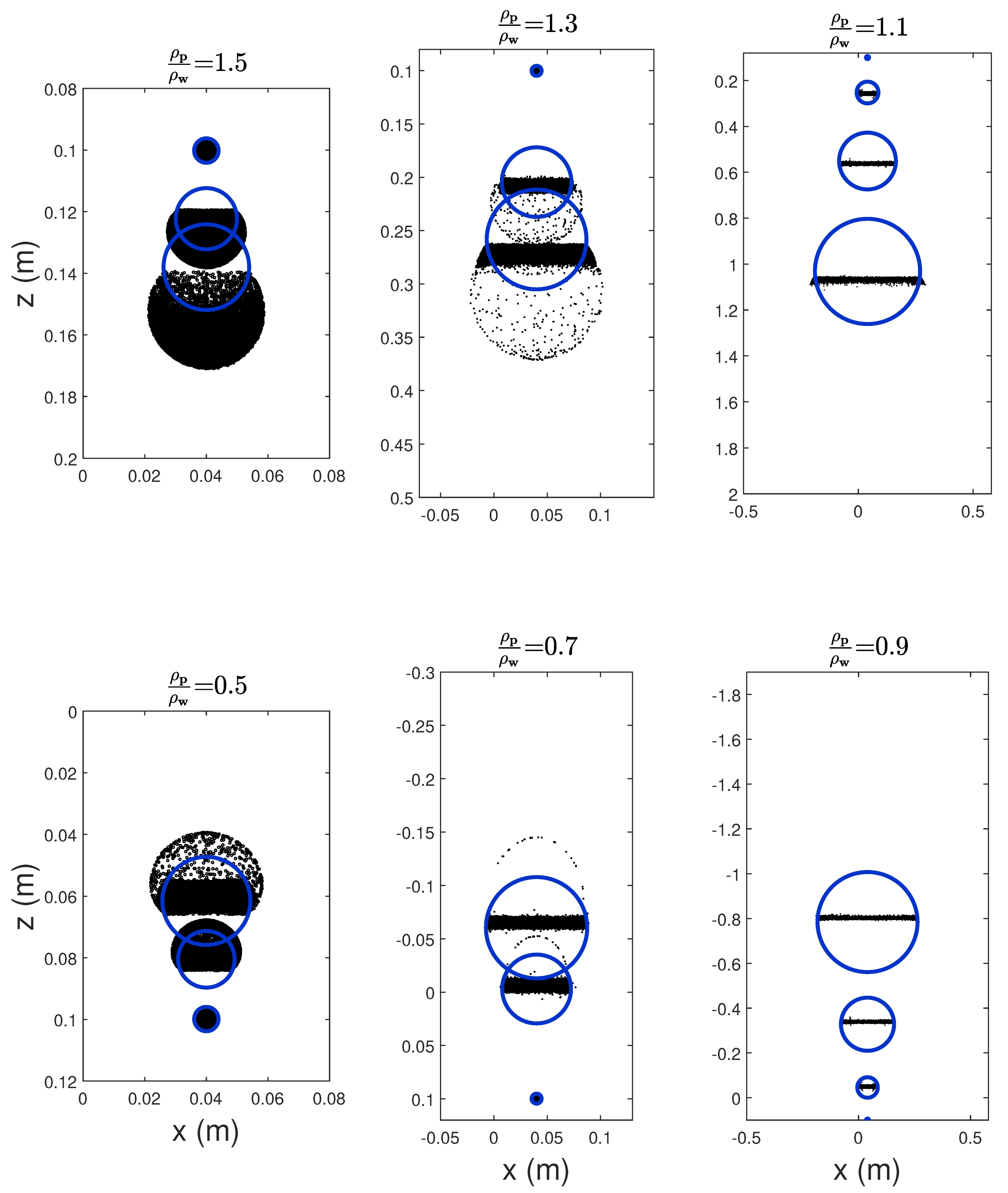
Figure 3 shows examples of particle clouds that are released from the rest for both positive and negative particles. In this case, the particle Reynolds number is , and the pictures show three distinct density ratios for negatively (1.5, 1.3, and 1.1) and positively (0.5, 0.7, and 0.1) buoyant particles. The simulations continue until all particles have left the cloud, which occurs when the total buoyancy of the cloud reaches zero. The initial total cloud buoyancy () is the same in all cases. The images show snapshots of both positive and negative clouds at the same time. It is worth noting that negatively buoyant particles exit the cloud more quickly than their positively buoyant counterparts.
At high-density ratios, such as 1.5 and 0.5, the particles initially remain together in the cloud as a single entity. Later, they precipitate in a swarm vortex ring shaped like a bowl. However, the particles stay in the cloud longer for small-density ratios like 1.1 and 0.9. This results in a significant increase in the cloud size due to entrainment. Eventually, the particles rain out of the cloud but dissipate differently from the swarm-shaped formation observed in high-density ratios.
For the intermediate density difference case (center column in Figure 3), some particles are ejected from the cloud at an early time and travel ahead of the cloud. However, the number ejected is much higher for the denser particles (top row with ) compared to the number initially ejected for the lighter particles (bottom row with ). This behavior is also observed to a greater or lesser extent for the other cases shown in Figure 3, though it is less clear in the two-dimensional plots of the three-dimensional flow for these cases.
4.3. Quantitative Results
To better compare positively and negatively buoyant cloud cases, we introduce a time and length scale based on cloud buoyancy and particle terminal velocity. The scales are given by
Based on these scales, several non-dimensional variables can be defined. These are as follows: the cloud buoyancy
travel time
cloud velocity
cloud radius
and cloud height
Figure 4 displays the dimensionless cloud buoyancy , velocity , and radius as a function of time for the cases shown in Figure 3. In all six cases, there is an initial ejection of a large number of particles (top row of Figure 4) followed by their re-entrainment into the cloud. For the lowest density difference (right-hand column), almost all the particles are re-entrained and remain within the cloud for a prolonged period before settling out. However, despite having the same terminal velocity, the denser (negatively buoyant) particles (red line) fall out much earlier than the lighter (positively buoyant) particles (blue line). For the larger density differences, the deviation between the red and blue lines occurs much sooner, as fewer of the denser particles are re-entrained back into the cloud following the initial ejection. Note that the ejection and re-entrainment cycle produces a significant oscillation in the cloud buoyancy () (Figure 4 middle column top row) but only a small amplitude fluctuation in the velocity (middle row), while the displacement plot is smooth (bottom row). This is because the buoyancy fluctuation is integrated over time to obtain the velocity. Also, the similarity solution to the single-phase buoyant cloud model indicates the velocity scales on the square root of the cloud buoyancy [12]. Therefore, the amplitude of the fluctuations in is attenuated in the velocity signal.
For each simulation listed in Table 1, the fraction of particles that remain within the cloud () are tracked over time. These data are plotted in Figure 5 for all the cases simulated. Each row of plots represents a pair of density ratios that produce the same initial conditions in every way except the sign of the buoyancy. Therefore, the only difference in behavior between each pair of plots is the sign of the particle buoyancy.
For the largest density difference particles, shown in the top row of Figure 5, there is a rapid decrease in the number of particles in the cloud as they are ejected from the vortex ring. This is particularly true for the denser particles (right-hand plot), where the vast majority of the particles are removed from the cloud by . For the cloud formed by lighter particles, this is also true for most particle Reynolds numbers. However, for the smallest particles, , the particles are constantly being ejected and re-entrained into the cloud as indicated by the oscillating line.
As the density difference between the particles and the ambient fluid decreases (lower rows), the time for particles to be fully removed increases. This is because the particle terminal velocity is smaller and it takes longer for the cloud to slow down to the terminal velocity of the particles. The same difference between heavy and light particles is still seen with the smaller lighter particles being re-entrained back into the cloud for longer periods of time compared to the equivalent denser particles. Further, as the density difference decreases, higher Reynolds number particles start to exhibit the ejection re-entrainment cycle. For , even some of the denser particles start to be re-entrained.
For the lowest density difference cases, and , a different behavior is observed. In these cases, some of the particles are initially ejected, but all particles are re-entrained and then remain circulating in the cloud for some time before eventually falling out of the cloud. However, as stated before, equivalent pairs of particles, that is the same , have the same terminal velocity, and each cloud has the same initial buoyancy. However, the denser particles leave the cloud sooner than the lighter particles. Therefore, this process is not due solely to the cloud velocity falling below the particle terminal velocity. If that were the case, the ejection height would be the same for heavy and light particles with the same Re and density difference.
One possible explanation for this difference in behavior is the response of the particles to being pushed along the curved streamlines of the spherical Hill’s vortex. The particles that are denser than the ambient fluid will find it harder to follow the curved path and will tend to move away from the center of curvature of the streamlines and out of the particle cloud, whereas the particles that are less dense will be drawn further into the cloud and have a longer residence time.
The results in Figure 5 indicate that, even for particle clouds that have a bulk density ratio that is relatively small, their behavior may differ significantly depending on whether or not the particle cloud is positively or negatively buoyant. That is, a particle cloud that would typically be regarded as Boussinesq based on its bulk density ratio will behave differently depending on whether the constituent particles are positively or negatively buoyant. This is even true for small particle density ratios. In the bottom row of Figure 5, the density ratios are and and the time at which all the particles have left the cloud is up to 60% longer for the positively buoyant (lighter) particles compared to the negatively buoyant (heavier) particles. As such, the behavior of the cloud depends on the direction of the sign of the buoyancy of the clouds. This is a hallmark of non-Boussinesq flows indicating that two-phase density-driven clouds never fully behave in line with the Boussinesq assumption.
5. Discussion and Conclusions
A model for particle clouds has been developed and validated by the numerical and experimental work of Lai et al. [16]. The cloud was modeled as a buoyant vortex ring, with the velocity field computed by approximating the buoyant vortex ring as an expanding Hill’s spherical vortex. The rate of growth of the cloud radius in the fluid phase is assumed to be a function of the entrainment coefficient, which is a function of the cloud number. This was obtained from the experimental work of Lai et al. [1]. The growth rate of the vortex ring in the subsequent dispersive regime was also obtained experimentally by Lai et al. [16]. The particle tracking equation is then used to track the motion of particles with different forces acting on them. The contribution of buoyancy of all particles inside the cloud is accounted for by summing the number of particles within the cloud at each time step. The model included a random walk turbulent dispersion term for the particles and was validated using previously published experimental data (see Figure 2).
The validated model was used to conduct a parametric study to examine the difference in behavior between clouds that are nominally identical other than the sign of the buoyancy term. Simulation results indicate that particles are ejected and/or fall out of the buoyant cloud more rapidly when they are denser than the ambient fluid compared to identical clouds wherein the particles are less dense than the ambient fluid (see Figure 5). This is even the case for the smallest density differences and lowest particle Reynolds numbers modeled. Therefore, even for cases where the particle settling velocity and density differences are small, the behavior of the cloud is quite different depending on the sign of the particle buoyancy.
This would suggest that the Boussinesq assumption may not be appropriate for such flows and that positively and negatively buoyant clouds will behave differently. This difference is due to the response of the particles to ejection and re-entrainment into the cloud. Denser particles are harder to re-entrain into the cloud because of their higher inertia. Another result of this study is that simplified modeling approaches that treat the sediment cloud as a continuum and assume that the particles are retained in the cloud until the cloud velocity falls below the settling velocity, may over-predict the time for particles to settle out because they do not model the ejection and re-entrainment process.
Therefore, it is important to understand the size distribution of dredged materials before making a decision about how to model the flow, as even fairly small particles with small density differences can result in flows that differ from continuum models even when the nominal conditions for the Boussinesq assumption have been satisfied.
Although this study modeled the formation of a particle cloud as a thermal, with a particle tracking model to quantify particle ejection and re-entrainment and a random walk model for both positive and negative particle clouds, this study assumed that the particles have the same diameters, that there are no collisions between particles, and that they can overlap on top of each other in the space domain. In future studies, the aim is to extend the model to the case of polydisperse particles and analyze elastic/inelastic collisions in three dimensions. There is also a clear need for more experimental studies over a broader range of parameters to identify the limitations of applying the Boussinesq assumption to sediment clouds.
Author Contributions
A.O.A. developed the numerical code that simulated the model, produced the results figures and collaborated with N.B.K. on the writing and problem conception and definition. N.B.K. suggested the initial topic for the study and collaborated with A.O.A. on the detailed problem conception, problem definition, model refinement, results presentation, and writing. A.A.K. worked on the initial problem development and writing. All authors have read and agreed to the published version of the manuscript.
Funding
This research received no external funding.
Data Availability Statement
The data present in this study are available on request from the first author.
Conflicts of Interest
The authors declare no conflicts of interest.
Nomenclature
| Latin Symbols | |
| B | Cloud buoyancy |
| Total particle buoyancy | |
| K | Dispersion coefficient |
| f | Particle force parameter |
| g | Gravitational acceleration |
| Cloud reduced gravity | |
| L | Length scale |
| Total particle mass | |
| Initial cloud momentum | |
| Cloud number | |
| Particle cloud radius | |
| Particle Reynolds number | |
| T | Time scale |
| Velocity of the cloud center | |
| Magnitude of the relative velocity of the particle and fluid | |
| Particle settling velocity | |
| , , | Particle velocity |
| , , | Fluid velocity within the cloud |
| Initial cloud volume | |
| V | Cloud volume |
| Horizontal cartesian coordinates | |
| , , | Particle location |
| z | Vertical coordinate |
| Vertical location of the cloud center | |
| Greek Symbols | |
| Entrainment coefficient | |
| Non-dimensional cloud buoyancy | |
| Time step | |
| Non-dimensional cloud height | |
| Non-dimensional cloud velocity | |
| Fraction of particles remaining in the cloud | |
| , , and | Drag coefficient parameters |
| Particle density | |
| Fluid density | |
| Non-dimensional time | |
| Kinematic viscosity of the fluid | |
| Normally distributed random variable | |
| Non-dimensional cloud radius |
References
- Lai, A.C.; Wang, R.Q.; Law, A.W.K.; Adams, E.E. Modeling and experiments of polydisperse particle clouds. Environ. Fluid Mech. 2016, 16, 875–898. [Google Scholar] [CrossRef]
- Polrot, A.; Kirby, J.; Birkett, J.; Sharples, G. Combining sediment management and bioremediation in muddy ports and harbours: A review. Environ. Pollut. 2021, 289, 117853. [Google Scholar] [CrossRef] [PubMed]
- Lohrer, A.M.; Wetz, J.J. Dredging-induced nutrient release from sediments to the water column in a southeastern saltmarsh tidal creek. Mar. Pollut. Bull. 2003, 46, 1156–1163. [Google Scholar] [CrossRef] [PubMed]
- Nayar, S.; Miller, D.; Hunt, A.; Goh, B.; Chou, L. Environmental effects of dredging on sediment nutrients, carbon and granulometry in a tropical estuary. Environ. Monit. Assess. 2007, 127, 1–13. [Google Scholar] [CrossRef] [PubMed]
- Manap, N.; Voulvoulis, N. Environmental management for dredging sediments–The requirement of developing nations. J. Environ. Manag. 2015, 147, 338–348. [Google Scholar] [CrossRef] [PubMed]
- Todd, V.L.; Todd, I.B.; Gardiner, J.C.; Morrin, E.C.; MacPherson, N.A.; DiMarzio, N.A.; Thomsen, F. A review of impacts of marine dredging activities on marine mammals. ICES J. Mar. Sci. 2015, 72, 328–340. [Google Scholar] [CrossRef]
- Bush, J.W.; Thurber, B.; Blanchette, F. Particle clouds in homogeneous and stratified environments. J. Fluid Mech. 2003, 489, 29–54. [Google Scholar] [CrossRef]
- Li, C.W. Convection of particle thermals. J. Hydraul. Res. 1997, 35, 363–376. [Google Scholar] [CrossRef]
- Rahimipour, H. Dynamic behavior of particle clouds. In Proceedings of the 11th Australian Fluid Mechanics Conference, University of Tasmania, Hobart, Australia, 14–18 December 1992. [Google Scholar]
- Zhao, B.; Law, A.W.; Eric Adams, E.; Shao, D.; Huang, Z. Effect of air release height on the formation of sediment thermals in water. J. Hydraul. Res. 2012, 50, 532–540. [Google Scholar] [CrossRef]
- Ruggaber, G.J. Dynamics of Particle Clouds Related to Open-Water Sediment Disposal. Ph.D. Thesis, Massachusetts Institute of Technology, Cambridge, MA, USA, 2000. [Google Scholar]
- Turner, J. Buoyant plumes and thermals. Annu. Rev. Fluid Mech. 1969, 1, 29–44. [Google Scholar] [CrossRef]
- Noh, Y. Sedimentation of a particle cloud across a density interface. Fluid Dyn. Res. 2000, 27, 129. [Google Scholar] [CrossRef]
- Zhao, B.; Law, A.; Lai, A.; Adams, E. On the internal vorticity and density structures of miscible thermals. J. Fluid Mech. 2013, 722, R5. [Google Scholar] [CrossRef]
- Gensheimer, R.J.; Adams, E.E.; Law, A.W. Dynamics of particle clouds in ambient currents with application to open-water sediment disposal. J. Hydraul. Eng. 2013, 139, 114–123. [Google Scholar] [CrossRef]
- Lai, A.C.; Zhao, B.; Law, A.W.K.; Adams, E.E. Two-phase modeling of sediment clouds. Environ. Fluid Mech. 2013, 13, 435–463. [Google Scholar] [CrossRef]
- Hu, J.; Xu, G.; Shi, Y.; Wu, L. A numerical simulation investigation of the influence of rotor wake on sediment particles by computational fluid dynamics coupling discrete element method. Aerosp. Sci. Technol. 2020, 105, 106046. [Google Scholar] [CrossRef]
- Balakin, B.V.; Hoffmann, A.C.; Kosinski, P.; Rhyne, L.D. Eulerian-Eulerian CFD model for the sedimentation of spherical particles in suspension with high particle concentrations. Eng. Appl. Comput. Fluid Mech. 2010, 4, 116–126. [Google Scholar] [CrossRef]
- Chan, S.N.; Lee, J.H. A particle tracking model for sedimentation from buoyant jets. J. Hydraul. Eng. 2016, 142, 04016001. [Google Scholar] [CrossRef]
- Sun, R.; Xiao, H. SediFoam: A general-purpose, open-source CFD–DEM solver for particle-laden flow with emphasis on sediment transport. Comput. Geosci. 2016, 89, 207–219. [Google Scholar] [CrossRef]
- Scorer, R.S. Experiments on convection of isolated masses of buoyant fluid. J. Fluid Mech. 1957, 2, 583–594. [Google Scholar] [CrossRef]
- Gu, J.; Li, C.W. Modeling instantaneous discharge of unsorted particle cloud in ambient water by an Eulerian—Lagrangian method. J. Hydraul. Res. 2004, 42, 399–405. [Google Scholar]
- Lai, A.C.; Zhao, B.; Law, A.W.K.; Adams, E.E. A numerical and analytical study of the effect of aspect ratio on the behavior of a round thermal. Environ. Fluid Mech. 2015, 15, 85–108. [Google Scholar] [CrossRef]
- Turner, J.S. Turbulent entrainment: The development of the entrainment assumption, and its application to geophysical flows. J. Fluid Mech. 1986, 173, 431–471. [Google Scholar] [CrossRef]
- Swamee, P.K.; Ojha, C.S.P. Drag coefficient and fall velocity of nonspherical particles. J. Hydraul. Eng. 1991, 117, 660–667. [Google Scholar] [CrossRef]
- Dietrich, W.E. Settling velocity of natural particles. Water Resour. Res. 1982, 18, 1615–1626. [Google Scholar] [CrossRef]
- Kitanidis, P.K. Particle-tracking equations for the solution of the advection-dispersion equation with variable coefficients. Water Resour. Res. 1994, 30, 3225–3227. [Google Scholar] [CrossRef]
Figure 1.
Schematic diagram showing the particle cloud falling and spreading out with the particles eventually falling out of the vortex.
Figure 1.
Schematic diagram showing the particle cloud falling and spreading out with the particles eventually falling out of the vortex.

Figure 2.
Transient depth and half-width of the particle cloud (in the entrained fluid phase). Lines prediction, symbols observation. Size A represents particles with a diameter of 0.725 mm, while size B represents particles with a diameter of 0.513 mm [16].
Figure 2.
Transient depth and half-width of the particle cloud (in the entrained fluid phase). Lines prediction, symbols observation. Size A represents particles with a diameter of 0.725 mm, while size B represents particles with a diameter of 0.513 mm [16].

Figure 3.
An example of model predictions for positively and negatively buoyant cloud particles with six different density ratios for . The particles are represented in black, while the blue color shows the particle cloud growing over time due to entrainment. Note that the vertical scales differ in each column in order to show the full behavior over time for each cloud.

Figure 4.
Dimensionless cloud buoyancy , velocity , and radius as a function of time for the cases shown in Figure 3.
Figure 4.
Dimensionless cloud buoyancy , velocity , and radius as a function of time for the cases shown in Figure 3.

Figure 5.
Dimensional cloud buoyancy , velocity , and radius for the cases shown in Figure 3.
Figure 5.
Dimensional cloud buoyancy , velocity , and radius for the cases shown in Figure 3.


Table 1.
List of density ratios and Reynolds numbers simulated.
| Buoyancy Sign | ||
|---|---|---|
| Positive | 0.9, 0.8, 0.7, 0.6, 0.5 | 0.48, 1.0, 1.56, 2.36, 12.76, 25.6, 43.5 |
| Negative | 1.1, 1.2, 1.3, 1.4, 1.5 | 0.48, 1.0, 1.56, 2.36, 12.76, 25.6, 43.5 |
Disclaimer/Publisher’s Note: The statements, opinions and data contained in all publications are solely those of the individual author(s) and contributor(s) and not of MDPI and/or the editor(s). MDPI and/or the editor(s) disclaim responsibility for any injury to people or property resulting from any ideas, methods, instructions or products referred to in the content. |
© 2024 by the authors. Licensee MDPI, Basel, Switzerland. This article is an open access article distributed under the terms and conditions of the Creative Commons Attribution (CC BY) license (https://creativecommons.org/licenses/by/4.0/).
Share and Cite
MDPI and ACS Style
Alnahit, A.O.; Kaye, N.B.; Khan, A.A. Understanding the Influence of the Buoyancy Sign on Buoyancy-Driven Particle Clouds. Fluids 2024, 9, 101. https://doi.org/10.3390/fluids9050101
AMA Style
Alnahit AO, Kaye NB, Khan AA. Understanding the Influence of the Buoyancy Sign on Buoyancy-Driven Particle Clouds. Fluids. 2024; 9(5):101. https://doi.org/10.3390/fluids9050101
Chicago/Turabian StyleAlnahit, Ali O., Nigel Berkeley Kaye, and Abdul A. Khan. 2024. "Understanding the Influence of the Buoyancy Sign on Buoyancy-Driven Particle Clouds" Fluids 9, no. 5: 101. https://doi.org/10.3390/fluids9050101