

A Novel Differentiated Control Strategy for an Energy Storage System That Minimizes Battery Aging Cost Based on Multiple Health Features
 ,
,
Abstract
:1. Introduction
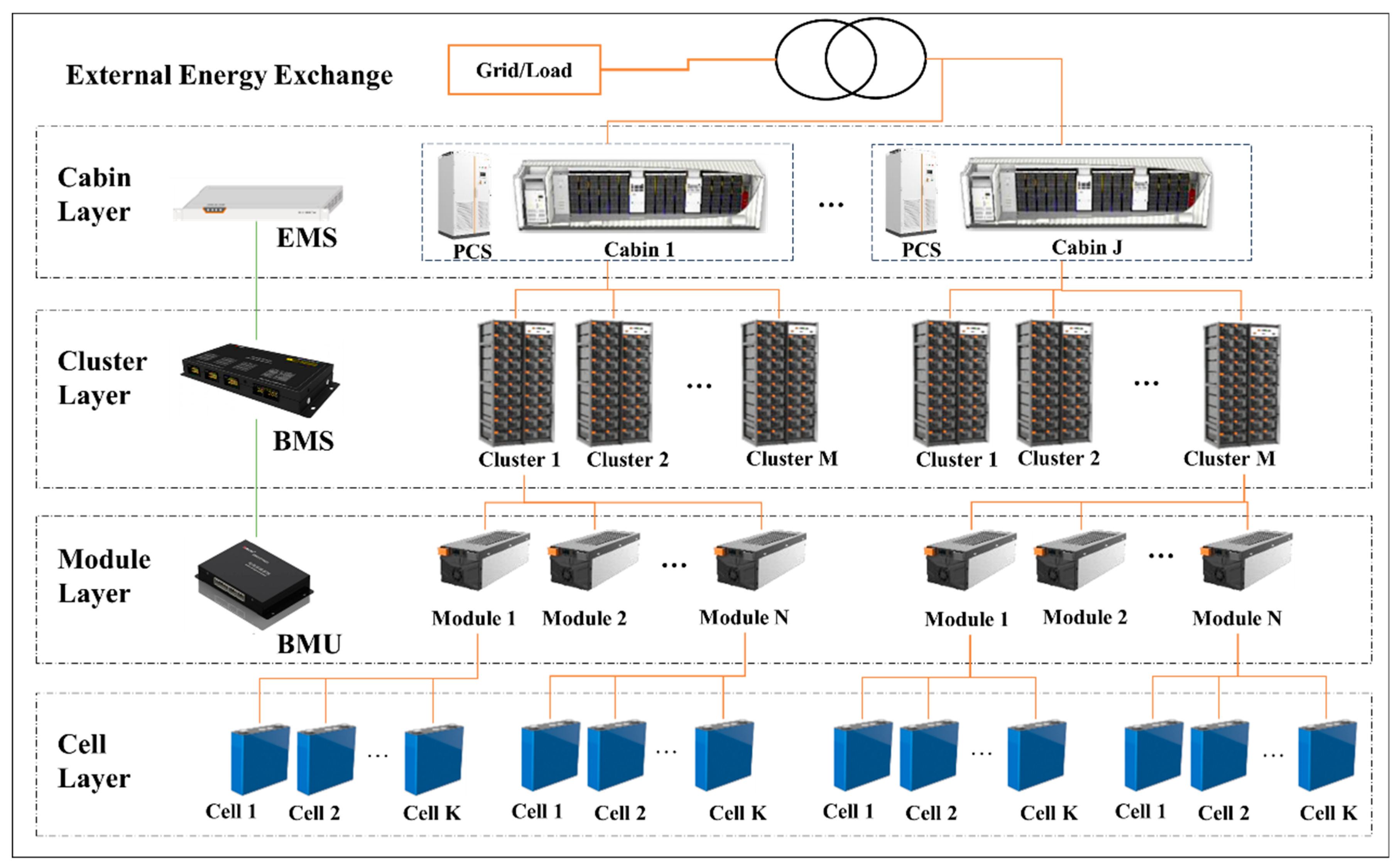
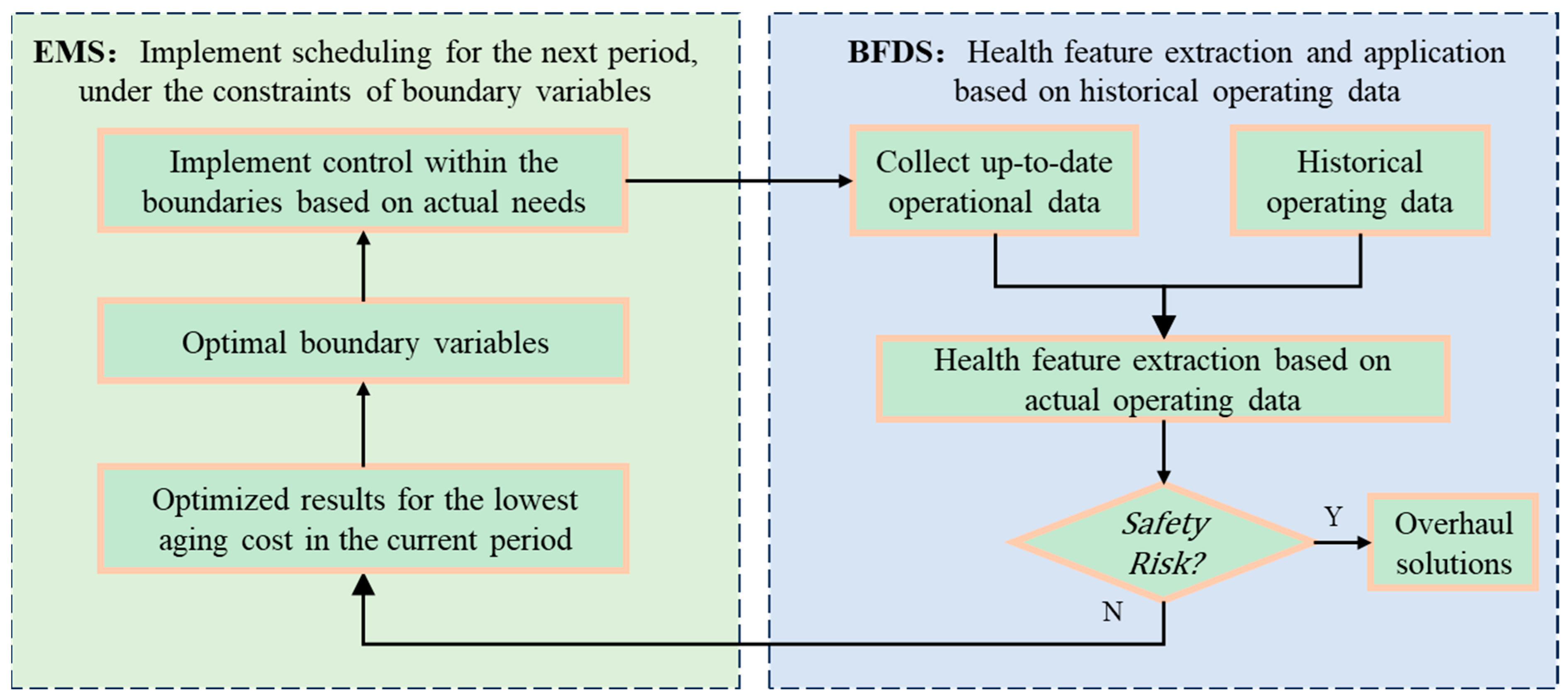
2. Control Strategy
2.1. Optimization Control Strategy to Minimize Aging Cost in a Single Operational Period
- (1)
- In the case of emergency batteries enabled, when other batteries are sufficient to take the place of E batteries, they will be reduced in power at a rate of 2%/s for transition into standby mode.
- (2)
- If other batteries reach the lower limit of the DOD, D and E will be enabled to fill the vacancy successively, to meet the requirements of charging and discharging instructions.
2.2. Rolling Optimization Process for Long-Time Operational Scenarios
3. Extraction and Prediction of Multi-Dimensional HFs
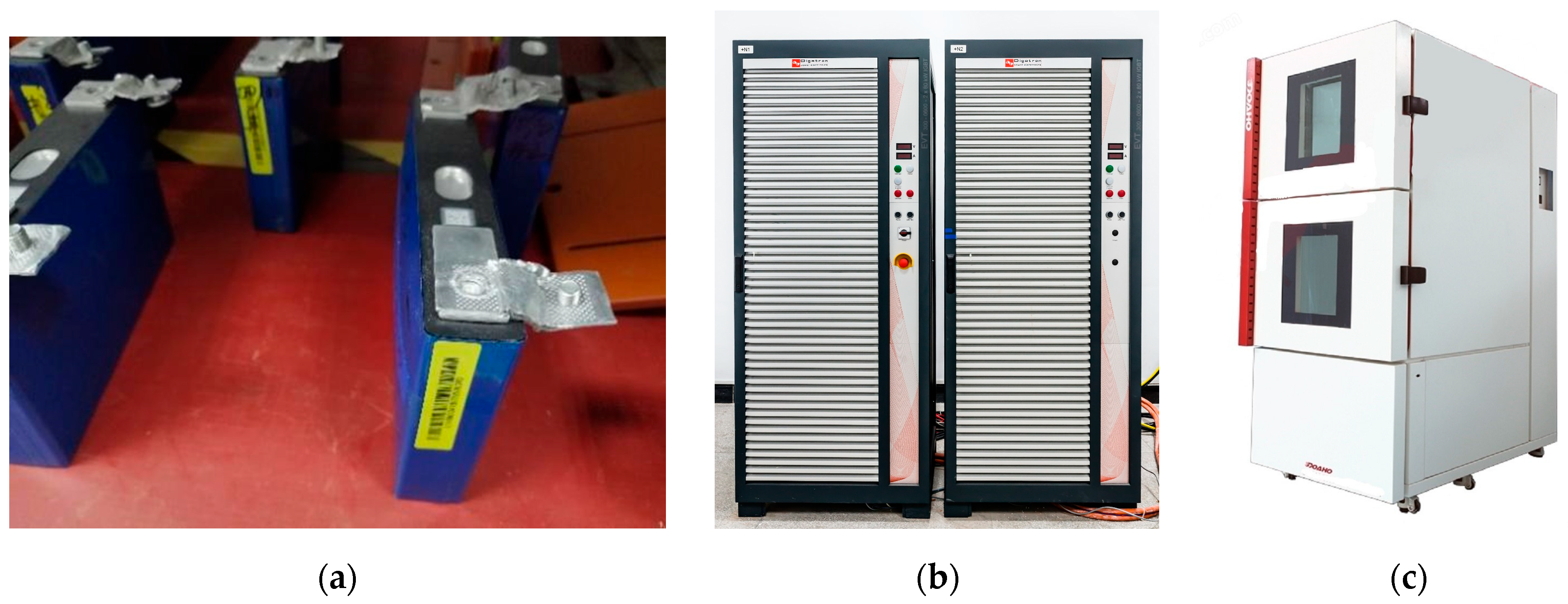
3.1. Aging Experiment
- Actual capacity test: Discharge the batteries at a constant current of 1/3C to the lower cut-off voltage of 2.75 V. Charge them at a constant current of 1/3C to 4.2 V, and subsequently charge at a constant voltage until the current drops below C/20. Next, discharge them at a constant current of 1/3C to the lower cut-off voltage of 2.75 V. Repeat this charge and discharge procedure two times. Refer to Figure 8a.
- Low-current discharge curve: Charge the batteries at a current of 1/3C to the cut-off voltage and discharge them at a current of C/20 to 2.75 V after standing, as shown in Figure 8b.
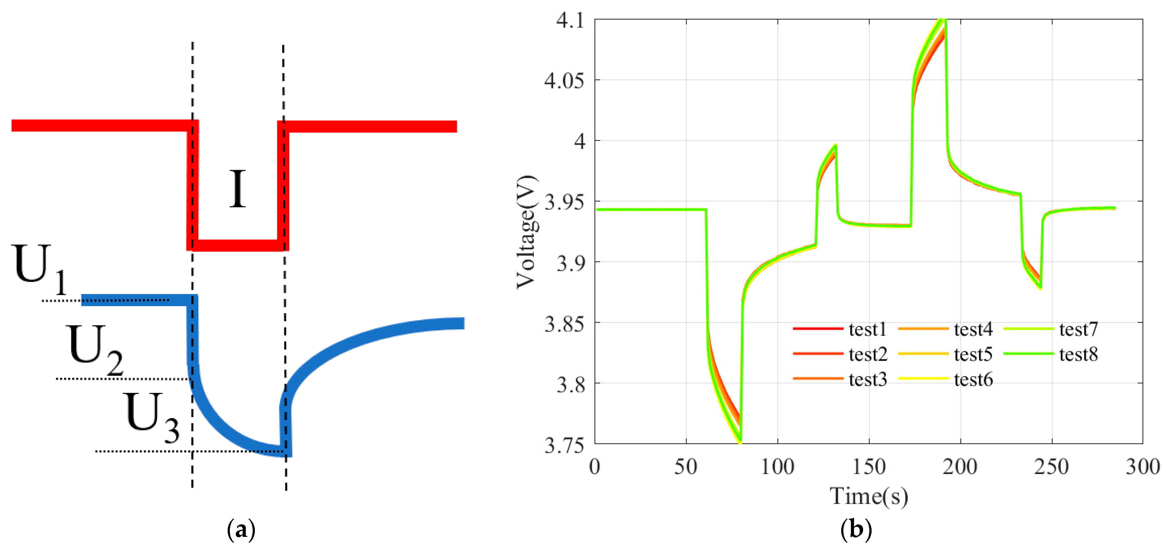
- HPPC: Perform tests at varying SOC levels [28]. After the batteries are fully charged, gradually discharge them to 80%, 60%, 50%, 40%, and 20% SOC for evaluations. Specifically, discharge them at a current of 2C for 18 s, after setting them aside to stand for 40 s, charge them at 1C for 10 s, and then set them aside again to stand for 40 s. Then charge the batteries with a current of 2C for 18 s, after setting them aside to stand for 40 s, discharge them at a current of 1C for 10 s, and finally set them aside to stand for 40 s. Refer to Figure 8e.
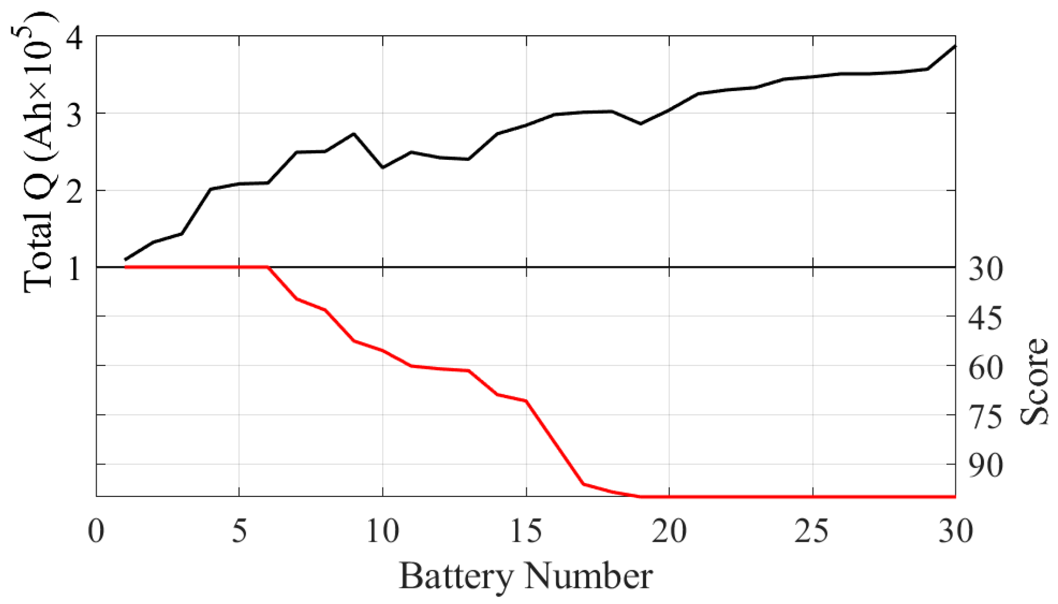
- Cyclic aging: Cyclic aging is performed according to the set DOD and C. No. 1 and No. 13 battery are plotted together to show the difference in performance between different batteries. Refer to Figure 8f.
3.2. Extraction of HFs
- Resistance. The ohmic and polarization internal resistances can be calculated through the HPPC test according to the literature [54]. Refer to Figure 12a and Formula (8). Figure 12b displays the HPPC curves for multiple tests of No. 1 battery, illustrating that voltage changes intensify under the same current excitation with aging progression. Figure 13 shows the change curves of ohmic and polarization internal resistances.
- 3.
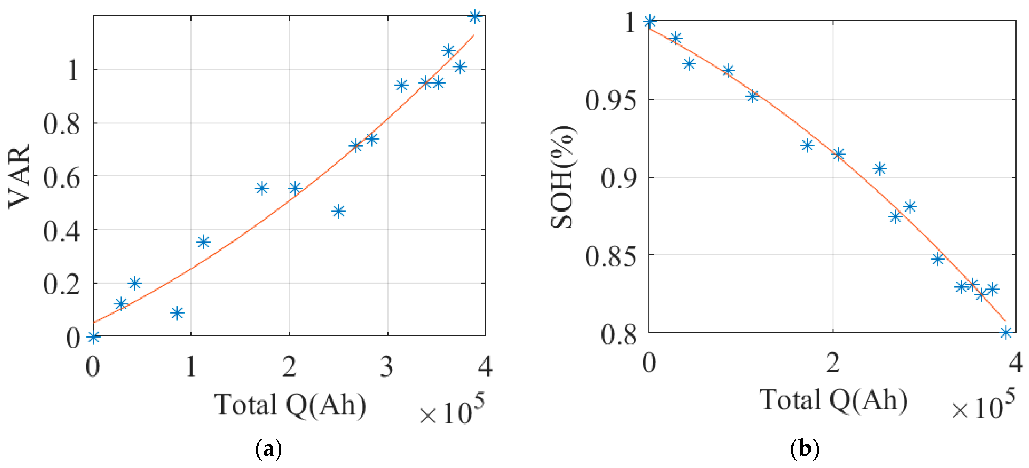
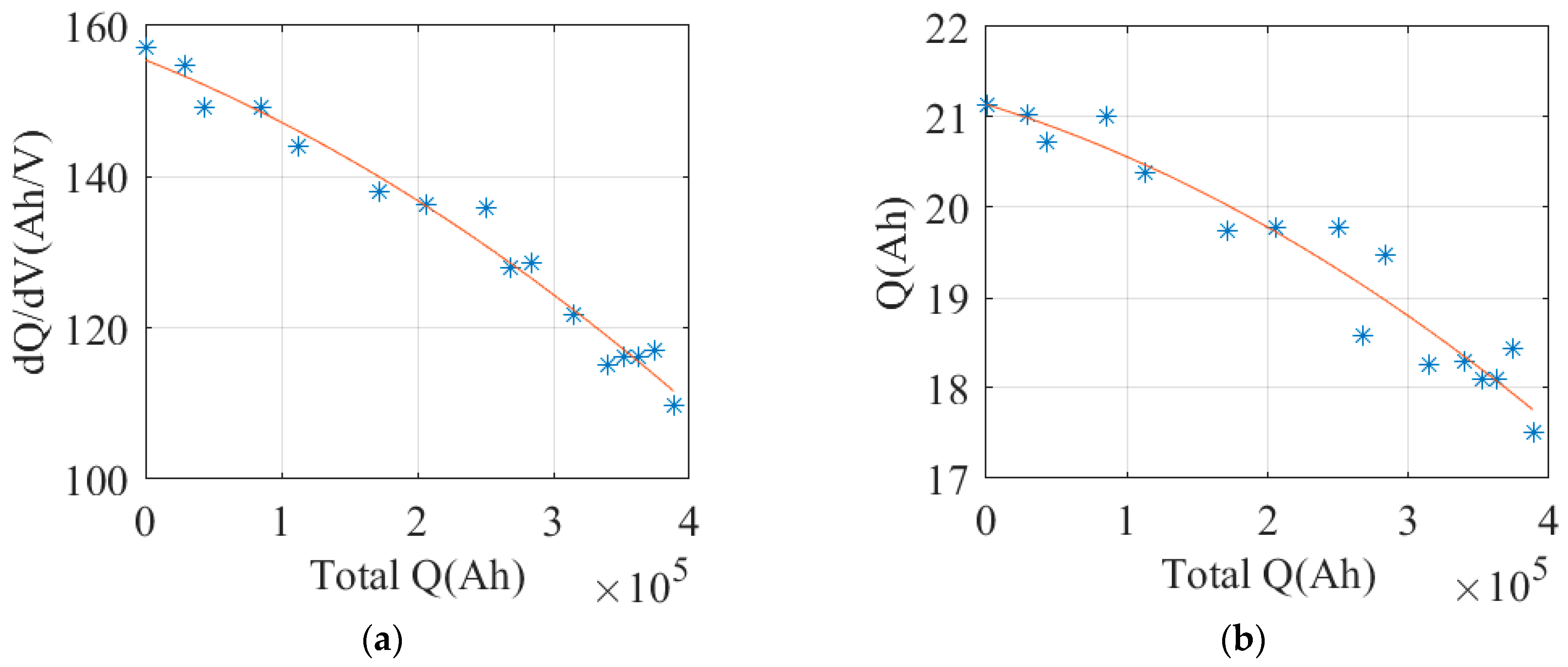
- ICA. Figure 14a shows the original IC curve of a single test, subjected to smoothing. Figure 14b shows the IC curves of multiple tests, indicating decreasing peak values, rightward shifting peak positions, and narrowed peak areas with aging progression. Figure 15 shows the variation curves of peak values and peak areas, respectively.
- 4.
- Relaxation. Relaxation refers to the process in which voltage slowly returns to a specific stationary stage upon the conclusion of excitation. The recovery to 3.91 V upon the conclusion of excitation was considered for current calculations. Figure 16 illustrates the recovery process following the removal of excitation during multiple HPPC tests. As shown, the recovery process is prolonged with aging progression. Figure 17 shows the variation curves of relaxation time and slope.
3.3. Prediction of HFs
4. Prediction Method of Aging Cost for Energy Storage System
5. Case Study
5.1. Description of Application Scenario
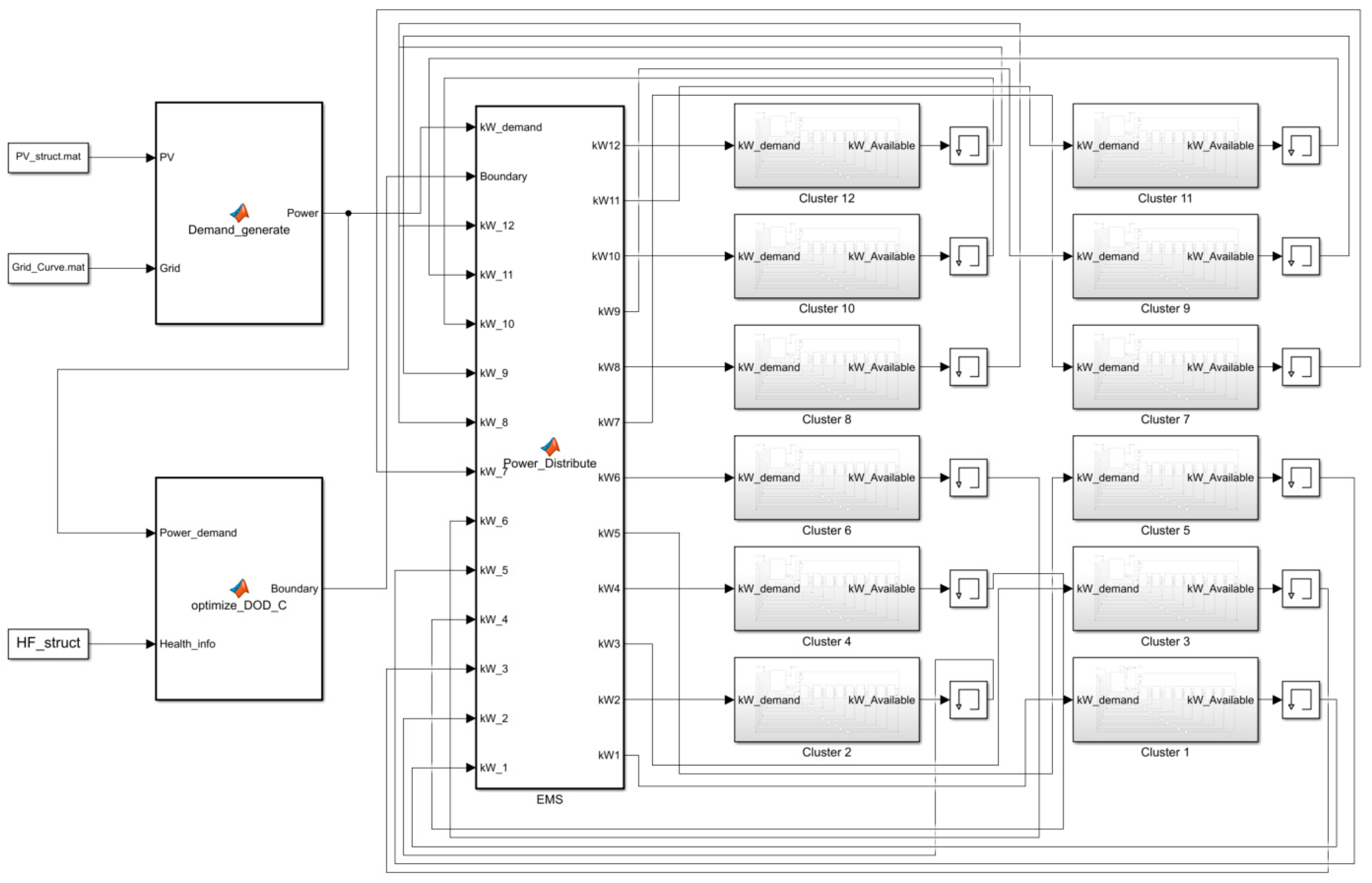
5.2. Simulation Model of Energy Storage System
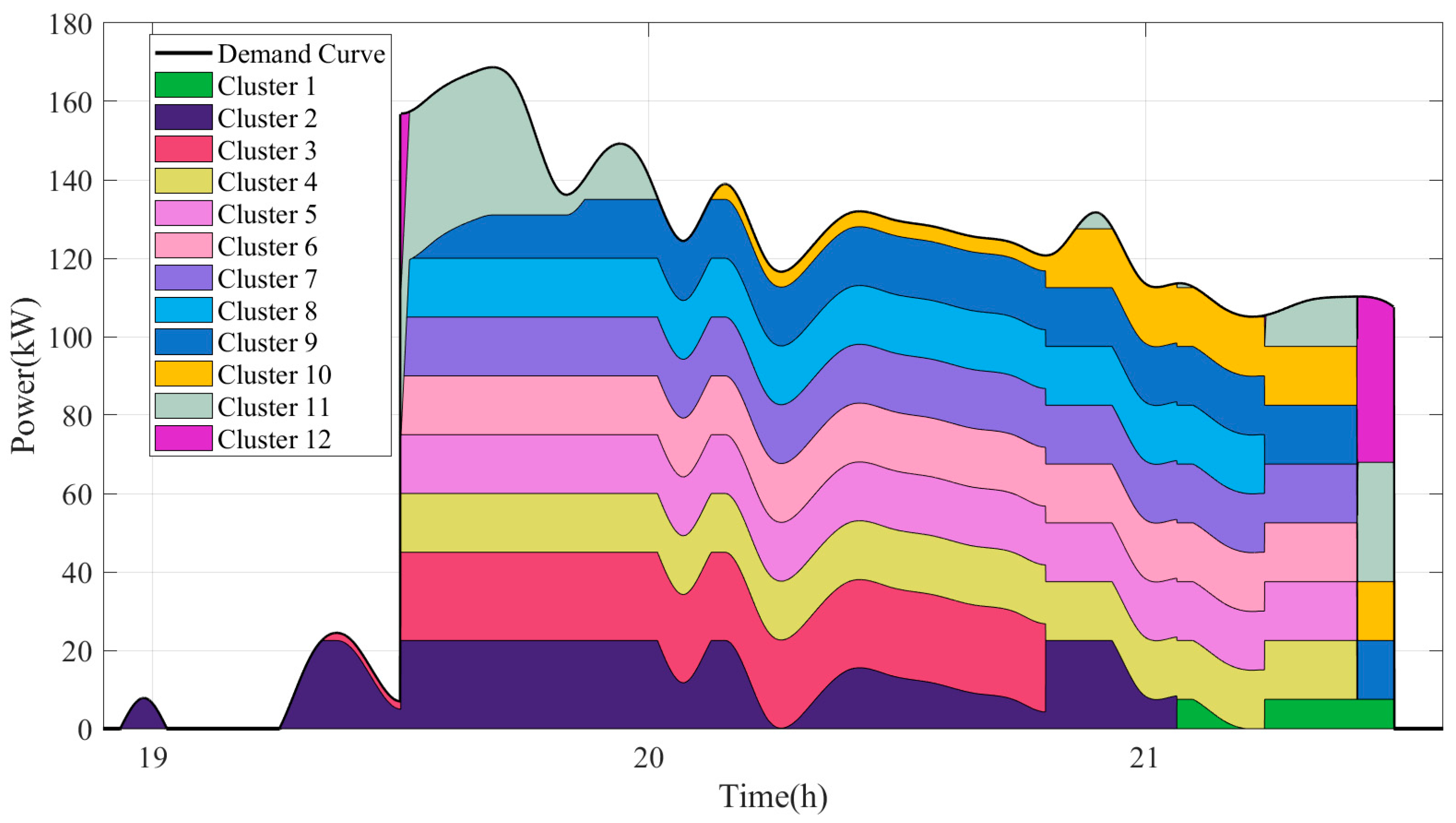
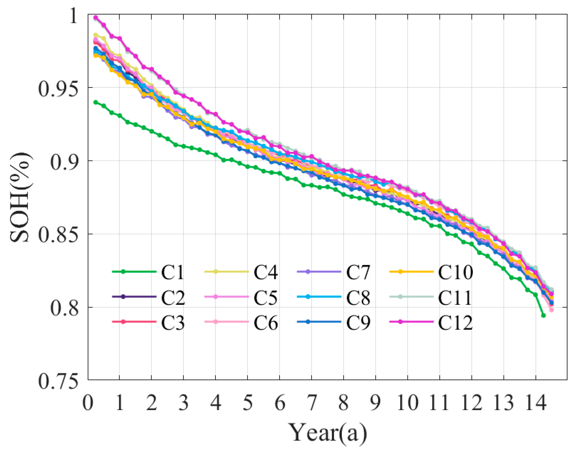
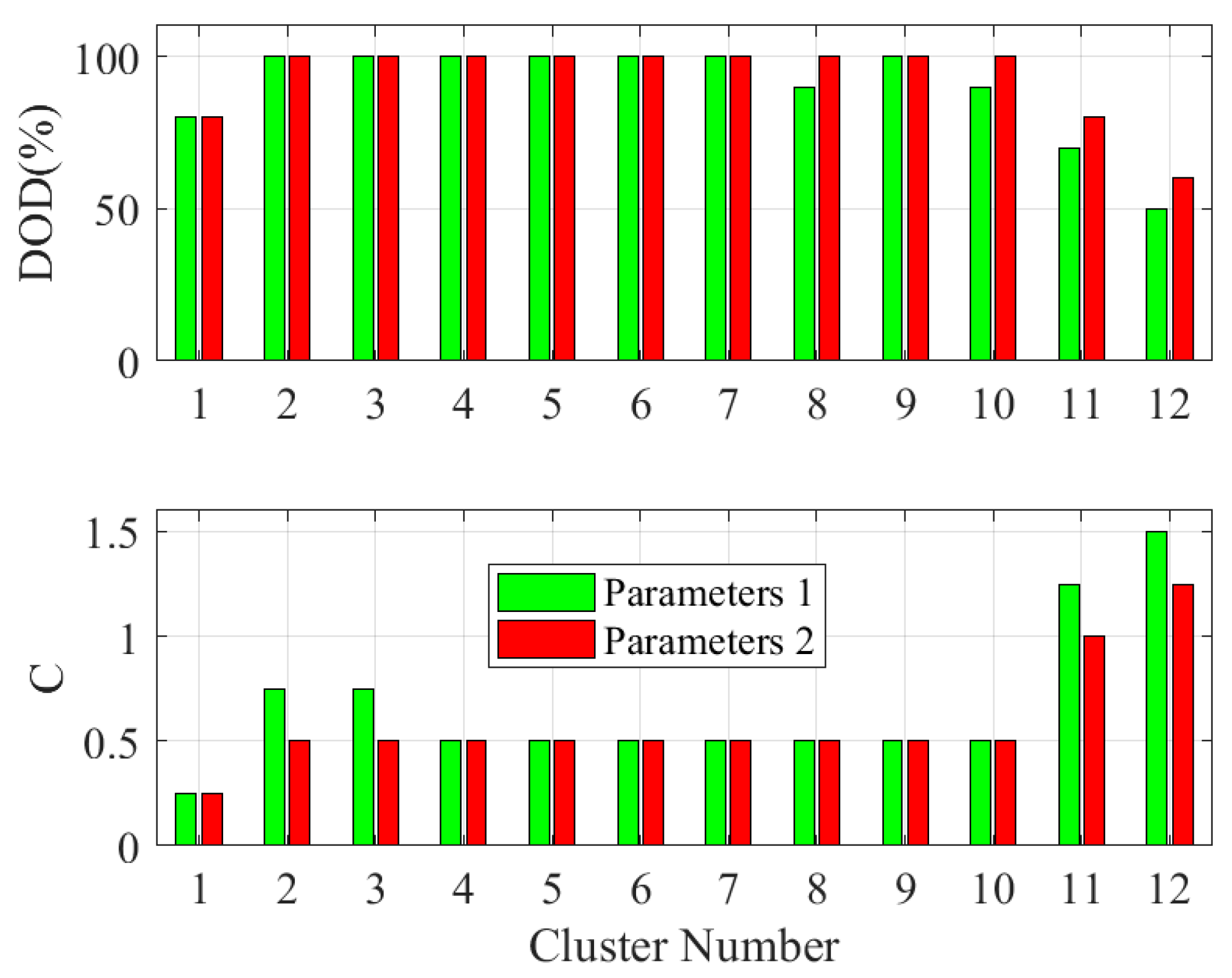
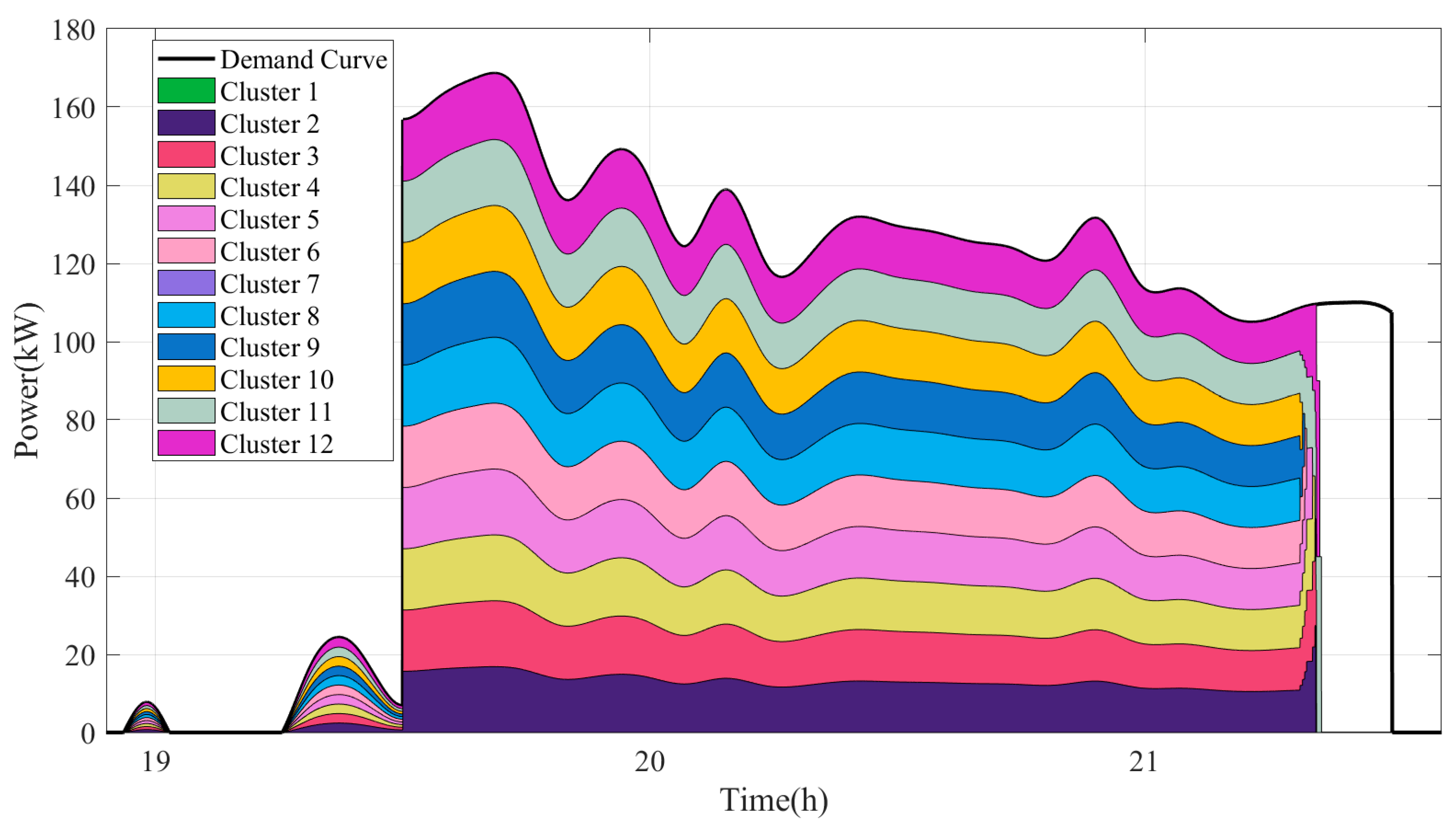
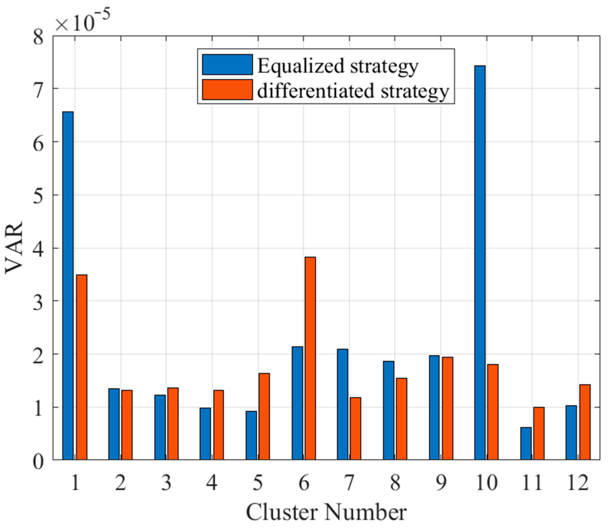
5.3. Comparative Analysis of Results
6. Conclusions
- The optimization control strategy presented, along with its solving process, helps in reducing aging costs and extending the service life of energy storage systems. Furthermore, it improves module consistency, offering advantages for cascade utilization following module recombination.
- The periodic rolling optimization mode proposed for integrating this strategy into engineering operation benefits not only from reducing the computational power needed for each optimization control but also from enabling iterative adjustments based on the actual operational status.
- The aging cost evaluation introduced incorporates multi-dimensional features, rather than solely considering capacity SOH.
- Due to time and equipment limitations, the comparative experiments were not sufficient. Variable intervals may be refined in the future, to establish a more accurate aging prediction model. Additionally, data collected during long-term operation revealed that batteries with high SOC and low operating frequency exhibited noticeable storage aging. In the subsequent strategy optimization, it may be beneficial to optimize SOC points after charging instead of performing a full charge each time.
- Utilizing the universality of the proposed approach, models can be developed with a small amount of experimental data in scenarios involving other types of batteries. These models can then be used for simulations of aging under multiple variables to provide a reference. This approach can help in reducing the cost associated with long-term aging experiments.
- Shortening the time span of each period allows for more refined optimization control in engineering applications. At the same time, we continue to explore other data-driven models to improve the effectiveness of the solution.
Author Contributions
Funding
Data Availability Statement
Acknowledgments
Conflicts of Interest
References
- Jia, J.; Hu, X.; Deng, Z.; Xiao, W.; Xu, H.; Han, F. Data-Driven Comprehensive Evaluation of Lithium-Ion Battery State of Health and Abnormal Battery Screening. J. Mech. Eng. 2021, 57, 141–149, 159. [Google Scholar] [CrossRef]
- Feng, F.; Hu, X.; Hu, L.; Hu, F.; Li, Y.; Zhang, L. Propagation Mechanisms and Diagnosis of Parameter Inconsistency within Li-Ion Battery Packs. Renew. Sustain. Energy Rev. 2019, 112, 102–113. [Google Scholar] [CrossRef]
- Hu, X.; Zhang, K.; Liu, K.; Lin, X.; Dey, S.; Onori, S. Advanced Fault Diagnosis for Lithium-Ion Battery Systems: A Review of Fault Mechanisms, Fault Features, and Diagnosis Procedures. IEEE Ind. Electron. Mag. 2020, 14, 65–91. [Google Scholar] [CrossRef]
- Jiang, X.; Jin, Y.; Zheng, X.; Hu, G.; Zeng, Q. Optimal Configuration of Grid-Side Battery Energy Storage System under Power Marketization. Appl. Energy 2020, 272, 115242. [Google Scholar] [CrossRef]
- Hu, X.; Xu, L.; Lin, X.; Pecht, M. Battery Lifetime Prognostics. Joule 2020, 4, 310–346. [Google Scholar] [CrossRef]
- Hassan, A.; Khan, S.A.; Li, R.; Su, W.; Zhou, X.; Wang, M.; Wang, B. Second-Life Batteries: A Review on Power Grid Applications, Degradation Mechanisms, and Power Electronics Interface Architectures. Batteries 2023, 9, 571. [Google Scholar] [CrossRef]
- Han, W.; Zou, C.; Zhou, C.; Zhang, L. Estimation of Cell SOC Evolution and System Performance in Module-Based Battery Charge Equalization Systems. IEEE Trans. Smart Grid 2019, 10, 4717–4728. [Google Scholar] [CrossRef]
- Zhao, Q.; Liao, K.; Yang, J.; He, Z.; Xu, Y. Aging Rate Equalization Strategy for Battery Energy Storage Systems in Microgrids. IEEE Trans. Smart Grid 2024, 15, 136–148. [Google Scholar] [CrossRef]
- Xu, B.; Zhao, J.; Zheng, T.; Litvinov, E.; Kirschen, D.S. Factoring the Cycle Aging Cost of Batteries Participating in Electricity Markets. IEEE Trans. Power Syst. 2018, 33, 2248–2259. [Google Scholar] [CrossRef]
- Luo, Y.; Tian, P.; Yan, X.; Xiao, X.; Ci, S.; Zhou, Q.; Yang, Y. Energy Storage Dynamic Configuration of Active Distribution Networks—Joint Planning of Grid Structures. Processes 2023, 12, 79. [Google Scholar] [CrossRef]
- Han, W.; Wik, T.; Kersten, A.; Dong, G.; Zou, C. Next-Generation Battery Management Systems: Dynamic Reconfiguration. IEEE Ind. Electron. Mag. 2020, 14, 20–31. [Google Scholar] [CrossRef]
- Yan, G.; Liu, D.; Li, J.; Mu, G. A Cost Accounting Method of the Li-Ion Battery Energy Storage System for Frequency Regulation Considering the Effect of Life Degradation. Prot. Control Mod. Power Syst. 2018, 3, 4. [Google Scholar] [CrossRef]
- Karunathilake, D.; Vilathgamuwa, D.; Mishra, Y.; Corry, P.; Farrell, T.; Choi, S.S. Degradation-Conscious Multiobjective Optimal Control of Reconfigurable Li-Ion Battery Energy Storage Systems. Batteries 2023, 9, 217. [Google Scholar] [CrossRef]
- Collath, N.; Tepe, B.; Englberger, S.; Jossen, A.; Hesse, H. Aging Aware Operation of Lithium-Ion Battery Energy Storage Systems: A Review. J. Energy Storage 2022, 55, 105634. [Google Scholar] [CrossRef]
- Gad, A.G. Particle Swarm Optimization Algorithm and Its Applications: A Systematic Review. Arch. Comput. Methods Eng. 2022, 29, 2531–2561. [Google Scholar] [CrossRef]
- Xiao, W.; Xu, H.; Jia, J.; Feng, F.; Wang, W. State of Health Estimation Framework of Li-on Battery Based on Improved Gaussian Process Regression for Real Car Data. IOP Conf. Ser. Mater. Sci. Eng. 2020, 793, 012063. [Google Scholar] [CrossRef]
- Liu, K.; Xiaopeng, T.; Teodorescu, R.; Gao, F.; Meng, J. Future Ageing Trajectory Prediction for Lithium-Ion Battery Considering the Knee Point Effect. IEEE Trans. Energy Convers. 2022, 37, 1282–1291. [Google Scholar] [CrossRef]
- Zhang, G.; Wei, X.; Tang, X.; Zhu, J.; Chen, S.; Dai, H. Internal Short Circuit Mechanisms, Experimental Approaches and Detection Methods of Lithium-Ion Batteries for Electric Vehicles: A Review. Renew. Sustain. Energy Rev. 2021, 141, 110790. [Google Scholar] [CrossRef]
- Zheng, Y.; Lu, Y.; Gao, W.; Han, X.; Feng, X.; Ouyang, M. Micro-Short-Circuit Cell Fault Identification Method for Lithium-Ion Battery Packs Based on Mutual Information. IEEE Trans. Ind. Electron. 2021, 68, 4373–4381. [Google Scholar] [CrossRef]
- Xiao, W.; Miao, S.; Jia, J.; Zhu, Q.; Huang, Y. Lithium-Ion Batteries Fault Diagnosis Based on Multi-Dimensional Indicator. In Proceedings of the 2021 Annual Meeting of CSEE Study Committee of HVDC and Power Electronics (HVDC 2021), Beijing, China, 28–30 December 2021; Volume 2021, pp. 96–101. [Google Scholar]
- Doostmohammadian, M.; Meskin, N. Sensor Fault Detection and Isolation via Networked Estimation: Full-Rank Dynamical Systems. IEEE Trans. Control Netw. Syst. 2021, 8, 987–996. [Google Scholar] [CrossRef]
- Gan, N.; Sun, Z.; Zhang, Z.; Xu, S.; Liu, P.; Qin, Z. Data-Driven Fault Diagnosis of Lithium-Ion Battery Overdischarge in Electric Vehicles. IEEE Trans. Power Electron. 2022, 37, 4575–4588. [Google Scholar] [CrossRef]
- Wu, C.; Zhu, C.; Ge, Y. A New Fault Diagnosis and Prognosis Technology for High-Power Lithium-Ion Battery. IEEE Trans. Plasma Sci. 2017, 45, 1533–1538. [Google Scholar] [CrossRef]
- Xia, B.; Chen, Z.; Mi, C.; Robert, B. External Short Circuit Fault Diagnosis for Lithium-Ion Batteries. In Proceedings of the 2014 IEEE Transportation Electrification Conference and Expo (ITEC), Dearborn, MI, USA, 15–18 June 2014; pp. 1–7. [Google Scholar]
- Wang, H.; Shi, W.; Hu, F.; Wang, Y.; Hu, X.; Li, H. Over-Heating Triggered Thermal Runaway Behavior for Lithium-Ion Battery with High Nickel Content in Positive Electrode. Energy 2021, 224, 120072. [Google Scholar] [CrossRef]
- Gao, Y.; Gao, Q.; Zhang, X. Study on Battery Direct-Cooling Coupled with Air Conditioner Novel System and Control Method. J. Energy Storage 2023, 70, 108032. [Google Scholar] [CrossRef]
- Doughty, D.H.; Crafts, C.C. FreedomCAR: Electrical Energy Storage System Abuse Test Manual for Electric and Hybrid Electric Vehicle Applications; Sandia National Laboratories (SNL): Albuquerque, NM, USA; Livermore, CA, USA, 2006. [Google Scholar]
- Białoń, T.; Niestrój, R.; Skarka, W.; Korski, W. HPPC Test Methodology Using LFP Battery Cell Identification Tests as an Example. Energies 2023, 16, 6239. [Google Scholar] [CrossRef]
- R-Smith, N.A.-Z.; Moertelmaier, M.; Gramse, G.; Kasper, M.; Ragulskis, M.; Groebmeyer, A.; Jurjovec, M.; Brorein, E.; Zollo, B.; Kienberger, F. Fast Method for Calibrated Self-Discharge Measurement of Lithium-Ion Batteries Including Temperature Effects and Comparison to Modelling. Energy Rep. 2023, 10, 3394–3401. [Google Scholar] [CrossRef]
- Wu, L.; Liu, K.; Liu, J.; Pang, H. Evaluating the Heat Generation Characteristics of Cylindrical Lithium-Ion Battery Considering the Discharge Rates and N/P Ratio. J. Energy Storage 2023, 64, 107182. [Google Scholar] [CrossRef]
- Steger, F.; Krogh, J.T.; Meegahapola, L.G.; Schweiger, H.-G. Calculating Available Charge and Energy of Lithium-Ion Cells Based on OCV and Internal Resistance. Energies 2022, 15, 7902. [Google Scholar] [CrossRef]
- Messing, M.; Shoa, T.; Habibi, S. Lithium-Ion Battery Relaxation Effects. In Proceedings of the 2019 IEEE Transportation Electrification Conference and Expo (ITEC), Detroit, MI, USA, 19–21 June 2019; pp. 1–6. [Google Scholar]
- Yu, P.; Wang, S.; Yu, C.; Shi, W.; Li, B. Study of Hysteresis Voltage State Dependence in Lithium-Ion Battery and a Novel Asymmetric Hysteresis Modeling. J. Energy Storage 2022, 51, 104492. [Google Scholar] [CrossRef]
- Wu, Z.; Yin, L.; Xiong, R.; Wang, S.; Xiao, W.; Liu, Y.; Jia, J.; Liu, Y. A Novel State of Health Estimation of Lithium-Ion Battery Energy Storage System Based on Linear Decreasing Weight-Particle Swarm Optimization Algorithm and Incremental Capacity-Differential Voltage Method. Int. J. Electrochem. Sci. 2022, 17, 220754. [Google Scholar] [CrossRef]
- Feng, X.; Merla, Y.; Weng, C.; Ouyang, M.; He, X.; Liaw, B.Y.; Santhanagopalan, S.; Li, X.; Liu, P.; Lu, L.; et al. A Reliable Approach of Differentiating Discrete Sampled-Data for Battery Diagnosis. eTransportation 2020, 3, 100051. [Google Scholar] [CrossRef]
- Noelle, D.J.; Wang, M.; Le, A.V.; Shi, Y.; Qiao, Y. Internal Resistance and Polarization Dynamics of Lithium-Ion Batteries upon Internal Shorting. Appl. Energy 2018, 212, 796–808. [Google Scholar] [CrossRef]
- Xiao, J.; Li, Q.; Bi, Y.; Cai, M.; Dunn, B.; Glossmann, T.; Liu, J.; Osaka, T.; Sugiura, R.; Wu, B.; et al. Understanding and Applying Coulombic Efficiency in Lithium Metal Batteries. Nat. Energy 2020, 5, 561–568. [Google Scholar] [CrossRef]
- Severson, K.A.; Attia, P.M.; Jin, N.; Perkins, N.; Jiang, B.; Yang, Z.; Chen, M.H.; Aykol, M.; Herring, P.K.; Fraggedakis, D.; et al. Data-Driven Prediction of Battery Cycle Life before Capacity Degradation. Nat. Energy 2019, 4, 383–391. [Google Scholar] [CrossRef]
- Maity, J.; Dutta, S.; Khanra, M. Constant Voltage Charging Curve Based Features and State of Health Estimation of Li-Ion Batteries: A Comprehensive Study. In Proceedings of the 2022 International Conference on Smart Generation Computing, Communication and Networking (SMART GENCON), Bangalore, India, 23–25 December 2022; pp. 1–7. [Google Scholar]
- Zheng, Y.; Han, X.; Lu, L.; Li, J.; Ouyang, M. Lithium Ion Battery Pack Power Fade Fault Identification Based on Shannon Entropy in Electric Vehicles. J. Power Sources 2013, 223, 136–146. [Google Scholar] [CrossRef]
- Gateman, S.M.; Gharbi, O.; Gomes de Melo, H.; Ngo, K.; Turmine, M.; Vivier, V. On the Use of a Constant Phase Element (CPE) in Electrochemistry. Curr. Opin. Electrochem. 2022, 36, 101133. [Google Scholar] [CrossRef]
- Xiong, R.; Sun, Y.; Wang, C.; Tian, J.; Chen, X.; Li, H.; Zhang, Q. A Data-Driven Method for Extracting Aging Features to Accurately Predict the Battery Health. Energy Storage Mater. 2023, 57, 460–470. [Google Scholar] [CrossRef]
- Zhang, K.; Xiong, R.; Qu, S.; Zhang, B.; Shen, W. Electrochemical Impedance Spectroscopy: A Novel High-Power Measurement Technique for Onboard Batteries Using Full-Bridge Conversion. IEEE Trans. Transp. Electrif. 2024. early access. [Google Scholar] [CrossRef]
- Tian, J.; Xiong, R.; Shen, W.; Lu, J. State-of-Charge Estimation of LiFePO4 Batteries in Electric Vehicles: A Deep-Learning Enabled Approach. Appl. Energy 2021, 291, 116812. [Google Scholar] [CrossRef]
- Mawonou, K.S.R.; Eddahech, A.; Dumur, D.; Beauvois, D.; Godoy, E. State-of-Health Estimators Coupled to a Random Forest Approach for Lithium-Ion Battery Aging Factor Ranking. J. Power Sources 2021, 484, 229154. [Google Scholar] [CrossRef]
- Jia, X.; Wang, S.; Cao, W.; Qiao, J.; Yang, X.; Li, Y.; Fernandez, C. A Novel Genetic Marginalized Particle Filter Method for State of Charge and State of Energy Estimation Adaptive to Multi-Temperature Conditions of Lithium-Ion Batteries. J. Energy Storage 2023, 74, 109291. [Google Scholar] [CrossRef]
- Lai, X.; Yuan, M.; Tang, X.; Zheng, Y.; Zhu, J.; Sun, Y.; Zhou, Y.; Gao, F. State-of-Power Estimation for Lithium-Ion Batteries Based on a Frequency-Dependent Integer-Order Model. J. Power Sources 2024, 594, 234000. [Google Scholar] [CrossRef]
- Liu, W.; Hu, X.; Lin, X.; Yang, X.-G.; Song, Z.; Foley, A.M.; Couture, J. Toward High-Accuracy and High-Efficiency Battery Electrothermal Modeling: A General Approach to Tackling Modeling Errors. eTransportation 2022, 14, 100195. [Google Scholar] [CrossRef]
- Zhou, H.; Gao, L.T.; Li, Y.; Lyu, Y.; Guo, Z.-S. Electrochemical Performance of Lithium-Ion Batteries with Two-Layer Gradient Electrode Architectures. Electrochim. Acta 2024, 476, 143656. [Google Scholar] [CrossRef]
- Jha, V.; Krishnamurthy, B. Modeling the SEI Layer Formation and Its Growth in Lithium-Ion Batteries (LiB) during Charge–Discharge Cycling. Ionics 2022, 28, 3661–3670. [Google Scholar] [CrossRef]
- Liu, D.; He, Y.; Chen, Y.; Cao, J.; Zhu, F. Electrochemical Modeling, Li Plating Onsets and Performance Analysis of Thick Graphite Electrodes Considering the Solid Electrolyte Interface Formed from the First Cycle. Electrochim. Acta 2023, 439, 141651. [Google Scholar] [CrossRef]
- Gu, Y.; Wang, J.; Chen, Y.; Xiao, W.; Deng, Z.; Chen, Q. A Simplified Electro-Chemical Lithium-Ion Battery Model Applicable for in Situ Monitoring and Online Control. Energy 2023, 264, 126192. [Google Scholar] [CrossRef]
- Luo, G.; Zhang, Y.; Tang, A. Capacity Degradation and Aging Mechanisms Evolution of Lithium-Ion Batteries under Different Operation Conditions. Energies 2023, 16, 4232. [Google Scholar] [CrossRef]
- Naylor Marlow, M.; Chen, J.; Wu, B. Degradation in Parallel-Connected Lithium-Ion Battery Packs under Thermal Gradients. Commun. Eng. 2024, 3, 2. [Google Scholar] [CrossRef]
- Liu, K.; Shang, Y.; Ouyang, Q.; Widanage, W. A Data-Driven Approach with Uncertainty Quantification for Predicting Future Capacities and Remaining Useful Life of Lithium-Ion Battery. IEEE Trans. Ind. Electron. 2021, 68, 3170–3180. [Google Scholar] [CrossRef]
- Fan, T.-E.; Liu, S.-M.; Yang, H.; Li, P.-H.; Qu, B. A Fast Active Balancing Strategy Based on Model Predictive Control for Lithium-Ion Battery Packs. Energy 2023, 279, 128028. [Google Scholar] [CrossRef]


| S | D | E | |
|---|---|---|---|
| D1 | D2 | D3 | |
| C1 | C2 | C3 |
| C | 1 | 1.2 | 1.5 | 2 | |
|---|---|---|---|---|---|
| DOD | |||||
| 30 | 1, 2 | 9, 10 | 17, 18 | 25, 26 | |
| 50 | 3, 4 | 11, 12 | 19, 20 | 27, 28 | |
| 70 | 5, 6 | 13, 14 | 21, 22 | 29, 30 | |
| 100 | 7, 8 | 15, 16 | 23, 24 | 31, 32 | |
| Extraction Method | HFs | Description |
|---|---|---|
| Measured data (applicable for cells, modules, and systems) | Self-discharge rate [29] | To identify serious energy loss. |
| Heat generation, temperature rise rate [30] | To identify temperature-related performance, such as serious self-heating and poor heat dissipation. | |
| Available charge/discharge capacity [31] | To diagnose failures such as energy response absence, excessive attenuation rate, and capacity diving. | |
| Relaxation-related features, such as recovery time, and recovery slope [32] | To diagnose reduced energy efficiency, insufficient power, etc. if there is failure to quickly return to normal after excitation. | |
| Hysteresis voltage [33] | To analyze whether the power performance degrades. | |
| Difference curves and associated features, such as incremental capacity analysis (ICA) [34], differential thermal voltammetry (DTV) [35] | To analyze performance details as a function of voltage, temperature, or pressure, such as power, energy, and heat production. | |
| Resistance, such as ohmic resistance, polarization resistance [36] | To analyze energy performance degradation and power performance degradation. | |
| Coulombic efficiency [37] | ||
| Description of the change in the charging curve, such as capacity variance (VAR) [1,38] | ||
| A series of features based on the constant current constant voltage (CCCV) curve [39] | ||
| Equivalent circuit model (applicable for cells and modules) | Resistance (R) [40], capacitance (C) [23], and constant phase element (CPE) [41] of equivalent resistance | To evaluate attenuation by comparing with relevant values of normal batteries of the same specification. |
| Experimental data | HPPC resistance [42] (applicable for cells and clusters) | To analyze power performance degradation |
| Electrochemical impedance spectroscopy (EIS parameters [43] (applicable for cells) | To reflect the physicochemical properties of internal materials and detect underlying failures from the perspective of impedances. | |
| Algorithm-based state estimation (applicable for cells, modules, and systems) | SOC [44], SOH [45], state of energy (SOE) [46], SOP [47], state of temperature (SOT) [48], etc. | To comprehensively analyze energy performance degradation and power performance degradation as a mature technique based on numerous studies. |
| Statistics on stacking relationship [20] (applicable for modules and systems) | Statistical analysis of extreme values and variances of voltage/temperature in modules | To screen abnormal cells or evaluate module consistency. |
| Statistical analysis of extreme values and variances of inter-cluster current | Screen abnormal clusters or evaluate cabin consistency. | |
| Various types of measurable data or HFs may be used to statistically analyze battery systems at different layers. | ||
| Electrochemical model (applicable for cells) | Physical and chemical parameters, such as maximum available lithium-ion concentration [49], solid electrolyte interface (SEI) film resistance [50], overpotential [51], resistance of components, and particle sizes of active materials [52] | To analyze energy and power attenuation and identify root causes based on electrochemical mechanisms [53]. |
| Simulation Round | Service Life (Quarterly) | Average Aging Cost (USD/kWh) | Inconsistency (Expressed as the Sum of Variances) | |
|---|---|---|---|---|
| Differentiated strategy on Mc_PSO | 1 | 58.0 | 0.0759 | 2.1821 × 10⁻⁴ |
| 2 | 54.0 | 0.0785 | 2.2413 × 10⁻⁴ | |
| 3 | 60.0 | 0.0749 | 2.0047 × 10⁻⁴ | |
| Mean | 57.3 | 0.0764 | 2.1427 × 10⁻⁴ | |
| Differentiated strategy on Ldw_PSO | 1 | 52.0 | 0.0806 | 2.6804 × 10⁻⁴ |
| 2 | 57.0 | 0.0776 | 2.3359 × 10⁻⁴ | |
| 3 | 59.0 | 0.0754 | 2.2033 × 10⁻⁴ | |
| Mean | 56.0 | 0.0779 | 2.4065 × 10⁻⁴ | |
| Equalized strategy | 1 | 50.0 | 0.0819 | 2.8150 × 10⁻⁴ |
| 2 | 49.0 | 0.0824 | 2.7615 × 10⁻⁴ | |
| 3 | 51.0 | 0.0812 | 2.6590 × 10⁻⁴ | |
| Mean | 50.0 | 0.0818 | 2.7452 × 10⁻⁴ |
Disclaimer/Publisher’s Note: The statements, opinions and data contained in all publications are solely those of the individual author(s) and contributor(s) and not of MDPI and/or the editor(s). MDPI and/or the editor(s) disclaim responsibility for any injury to people or property resulting from any ideas, methods, instructions or products referred to in the content. |
© 2024 by the authors. Licensee MDPI, Basel, Switzerland. This article is an open access article distributed under the terms and conditions of the Creative Commons Attribution (CC BY) license (https://creativecommons.org/licenses/by/4.0/).
Share and Cite
Xiao, W.; Jia, J.; Zhong, W.; Liu, W.; Wu, Z.; Jiang, C.; Li, B. A Novel Differentiated Control Strategy for an Energy Storage System That Minimizes Battery Aging Cost Based on Multiple Health Features. Batteries 2024, 10, 143. https://doi.org/10.3390/batteries10040143
Xiao W, Jia J, Zhong W, Liu W, Wu Z, Jiang C, Li B. A Novel Differentiated Control Strategy for an Energy Storage System That Minimizes Battery Aging Cost Based on Multiple Health Features. Batteries. 2024; 10(4):143. https://doi.org/10.3390/batteries10040143
Chicago/Turabian StyleXiao, Wei, Jun Jia, Weidong Zhong, Wenxue Liu, Zhuoyan Wu, Cheng Jiang, and Binke Li. 2024. "A Novel Differentiated Control Strategy for an Energy Storage System That Minimizes Battery Aging Cost Based on Multiple Health Features" Batteries 10, no. 4: 143. https://doi.org/10.3390/batteries10040143