Logic Solver Diagnostics in Safety Instrumented Systems for Oil and Gas Applications

Abstract

A safety instrumented system (SIS) is a complex unit composed of a set of hardware and software controls which are expressly used in critical process systems. A SIS should be specifically designed to obtain the failsafe state of the monitored plant or maintain safety of the procedure or a process when unacceptable or dangerous conditions occur. This paper focuses on condition monitoring and different diagnostic solutions used in safety instrumented systems, such as limit alarm trips, on-board diagnostics, and logic solver diagnostics. A case study consisting of the design of a safety loop using standard IEC 61508 for a complex safety instrumented system in the oil and gas field is presented in the paper using a diagnostics-oriented approach. The presented methodology aims at reaching the optimal tradeoff between IEC 61508 and the market requirements focusing on the best technological solutions to optimize diagnostics and safety and minimize the system’s response time in case of failure. The results of the application emphasize the importance of an accurate diagnostic strategy on safety instrumented systems for oil and gas plants.

1. Introduction

Condition monitoring (CM) is the process of monitoring one or more condition parameters in a system or machinery in order to identify some changes that are indicative of an incipient fault or, alternatively, imminent degradation of the equipment health (for more information see [1,2,3,4]). In the past, condition monitoring was applied simply through manual diagnostic actions. Nowadays, with the introduction of low-cost sensors and automated monitoring systems, online condition monitoring is rapidly growing. Condition monitoring strategies help select parameters from the sensors installed in the system in order to detect a change in the machine’s health condition [5,6,7]. This procedure is the core of predictive maintenance policies. As a matter of fact, the use of CM provides all the necessary information to schedule maintenance activities promptly and prevent unexpected failures [8,9,10,11,12]. Thus, cost reduction is guaranteed, maximizing the system uptime and optimizing the production efficiency. The added values of online rather than offline condition monitoring and manual data collection are listed below:

• Workforce optimization: manual diagnostics requires time and resource allocation to analyze the collected data and assess the required maintenance targets.
• Increased data storage: online monitoring guarantees continuous measurements for any piece of machinery, avoids mistakes in the registration of values and creates a trustworthy database.
• Improved diagnostics: great accuracy in failure prediction is achievable thanks to the unique database for historical trends and baseline data.
• Cost reduction: even if online diagnostics requires expensive software and application devices, the cost of manual diagnostics is considerably higher due to the personnel and time required, effectiveness of the implemented solutions, possibility of human errors, cost, and productivity impact of undiagnosed outage, etc.

Condition monitoring techniques are widely used on rotating equipment and other machinery (e.g., pumps, electric motors, and engines). The most popular methods used in modern industries to monitor the health state of such devices are vibration analysis, oil analysis, thermal analysis, power consumption analysis, and ultrasound analysis (see, for instance, but not only, [13,14,15,16,17]). Effectiveness and efficiency of condition monitoring remarkably depend on the application field. It seems obvious that monitoring the health state of a complex system to anticipate the occurrence of failures avoiding unexpected productivity outage allows achieving high availability with lower costs. However, a cost–benefit analysis is required to evaluate the proper effectiveness of CM in each field. For instance, a modern study emphasizes that the repayment period of a condition monitoring system for remote maintenance of a power plant is one single maintenance mission, reaching an estimated economic benefit of approximately 45 million euros after 10 maintenance missions [18].

This paper deals with the possible diagnostic solutions that could be implemented to improve the performances of safety instrumented systems (SIS) and thus guarantee adequate levels of the RAMS (reliability, availability, maintainability, and safety) parameters in the oil and gas industry.

Diagnostics and RAMS analysis are fundamental and critical aspects at oil and gas plants due to several different types of accidents and problems that have occurred over the years. Just to cite one of the major worldwide disasters in this field, Piper Alpha offshore disaster (1988, UK) resulted in 167 deaths and an approximate loss of $3.4 billion [19,20]. Taking 2012 as an example, 88 fatalities occurred in 52 separate incidents worldwide at onshore and offshore oil and gas plants. In addition, in the same year, 1699 injuries were reported in at least one day of work, with 53,325 lost workdays in total and billions of dollars of production losses [19]. Such examples allow to easily understand the crucial role that SIS and, more generally, functional safety play in the oil and gas industry in terms of human safety, productivity, environment safety and profits [20].

Consequently, the aim of the paper was to design and develop a safety instrumented system taking into account online diagnostic solutions for the oil and gas field. The main contribution of the presented methodology is the ability to reach the optimal tradeoff between the procedure defined in the international standards and the market requirements using a diagnostic solution in order to maximize risk reduction and increase the safety performance. The design of a SIS is a critical and crucial task in oil and gas applications, as well as in any other application fields. Usually, the design is performed following the guidelines of adequate international standards. From this point of view, the major gap that needs to be addressed is a lack of clarity and exhaustive explanation of the procedures contained in the standards for every possible system architecture, with particular reference to diagnostics-oriented solutions. This paper allows filling this gap with a step-by-step application to a real case study for the oil and gas industry. Furthermore, the paper emphasizes the need in a proper and accurate estimation of the reliability performance (e.g., in terms of the failure rate classification) for every item that makes up the SIS.

This paper is structured as follows: Section 2 presents the proposed diagnostic solutions to monitor the health state of the safety instrumented systems used in oil and gas applications. Section 3 illustrates the phases required to carry out a proper and accurate diagnostics-oriented design of a SIS. Finally, Section 4 presents the results of an actual application in which a safety instrumented system for the oil and gas industry is designed taking into account the diagnostics-oriented approach. The results emphasize how the implementation of an accurate diagnostic solution can help to reach the safety integrity level (SIL) determined during the specification phase.

2. Diagnostic Solutions for Safety Instrumented Systems

Many devices used in oil and gas applications are two-wire 4–20 mA sensor assemblies made of one or more sensing devices (i.e., thermocouples or RTDs in temperature instruments) and one dedicated transmitter to communicate with the system control panel. In many cases, the sensor’s output can vary in response to changes in the monitored physical quantity or in case of failure. These two latter conditions must be distinguished by dedicated diagnostic units. This section describes the possible alternative solutions to effectively and efficiently implement diagnostic and condition monitoring techniques in safety instrumented systems, with particular reference to the oil and gas industry [21].

2.1. Limit Alarm Trips

A limit alarm trip is one of the simplest and most important applications of condition monitoring in oil and gas systems. This procedure processes the signals provided by temperature, pressure, level, or flow sensors and compares them against a preset limit. In case the process signal goes to an undesirable high or low condition, the limit alarm activates a relay output to warn of the upcoming issue, provide on/off control or command an emergency shutdown. There are usually two types of alarm:

• Hard alarm: it is an independent limit alarm trip hardwired into the process and it is usually implemented on the output of a relay.
• Soft alarm: it is a software-implemented alarm based on DCS (distributed control systems) or PLC (programmable logic controllers).

In many applications, alarm functions are performed by “soft” practices; however, “hard” ones are widely used to implement low-cost redundancy, simple control, and backup of DCS and PLC strategies in critical emergency shutdowns and safety-related systems (SRSs). Soft alarms, in fact, are susceptible to common-mode failures while hard alarms are not exposed since they are independent from the DCS or PLC. Furthermore, hard alarms provide continuous supervision of the individual monitored process while soft practices perform intermittent scanning [22,23].

Limit alarm trips can provide many different actions, from a simple annunciation of a process’ unexpected behavior to a system emergency shutdown. The alarm trip receives input signals from a monitoring or control instrument and, in case the monitored process variable moves outside the setpoint, the alarm trip command a preset action. There are two thresholds, high and low, associated with the preset high and low alarm points. Usually, the alarm condition is maintained until the process signal moves back to the “normal running” values and passes out the dead band (i.e., the measurement range to reset the device and restore the “nonalarm” state). There are two thresholds, high and low, associated with the preset high and low alarm points. Figure 1 shows the output signal of a generic sensor (i.e., the input signal of the condition monitoring tool) as a function of time. The horizontal lines represent the high/low alarm trip levels and the high/low alarm trip resets. The bold line highlights the time in case the signal crosses the alarm level and the alarm state is active.

2.2. On-Board Diagnostics

If the sensor is equipped with a customized on-board diagnostic circuit, the device itself communicates its health status to the processing unit using dedicated communication channels or out-of-range outputs [24,25].

The main communication protocols are as follows: Highway Addressable Remote Transducer HART^® (a hybrid protocol fully compatible with 4–20 mA wiring focused on bringing digital information maintaining compatibility with this electrical standard) and Foundation Fieldbus FF (a distributed control system based on a multidrop bus focused on bringing the control architecture to the bus and bringing down the control to the device level). Both these communication protocols bring significant benefits to the manufacturing process [26,27]. HART^® and FF are proper solutions for configuration, calibration, diagnostics, and viewing internal variables. The major difference between these two protocols is that FF is also used for real-time closed-loop control. In fact, FF is completely digital end-to-end, from the sensor to the actuator, and it has several benefits over loops using hardwired 4–20 mA wiring and on/off signals [28,29]. The wiring connections of the 4–20 mA HART^® communication protocol are illustrated in Figure 2a, while Figure 2b shows the connections for Foundation Fieldbus [30,31].

2.3. Logic Solver Diagnostics

Condition monitoring is applied to the logic solver in case field sensors are not equipped with on-board diagnostics or the HART^® protocol is not used. The processor unit analyses measure trends or compares different data coming from multiple units (in case of redundant configuration). In case the process signal overcomes an undesirable high or low level, the logic solver performs the safety loop (e.g., emergency shutdown, on/off control, or warning relay output activation). The control implementation is generally linked to different thresholds that are upper and lower limits of the physical quantity under test. Throughout an ordinary operation, these thresholds are used to define the operative range; in case the measurement crosses those values, the control panel triggers the loop following the implemented logic.

In oil and gas applications, the most common sensors (i.e., temperature, level, flow, pressure) are usually monitored in compliance with a four-threshold technique, as in Figure 3:

• H: high threshold
• L: low threshold
• HH: high–high threshold
• LL: low–low threshold

“H” and “L” threshold crossing generally causes a visual alarm on the control panel in order to make the operator aware of the problem. In their turn, “HH” and “LL” threshold crossing is associated with more dangerous conditions: they lead to a progressive load reduction and gradual system shutdown or to an emergency shutdown that instantly stops the machine, in case of an extremely critical loop (generally associated with a concrete risk for the environment, health and safety of operators).

Field sensors can be affected by different types of failures that underline the importance of diagnostics to detect failures and guarantee safe system operation. The most common failure modes of field sensors are described as follows [32,33]:

• Out-of-calibration: field sensors must be calibrated against a known standard, but only short-term stability is checked during calibration; long-term stability should be monitored and determined by the user. This kind of failure can be observed instantly after installation (faulty assembly) or during device operation.
• Out-of-range: sensor failure is usually detected by performing a range check of device outcomes: all incoming values are checked against a given range by the logic solver. Sensor values that are outside that range are assumed to be incorrect and the device is considered to be out of order. High, low, and no output fall into this category.
• Stack-in-range: sensors are usually designed to fail out of range and this failure mode is quite rare but cannot be ignored anyway. When a stack-in-range failure occurs, sensor outcome is fixed inside the standard range of operation; for this reason, this failure mode is undetectable by the control logic without dedicated on-board diagnostics.
• Drift: signal drift follows a gradual and incremental trend towards the upper/lower limit of the operative range; for this reason, drift failures are critical since control logic cannot be aware of failure occurrence until device output goes out of range (in the absence of on-board diagnostics). Drift can occur very slowly, and that period of time is rather critical because control logic is using wrong values coming from a faulty sensor.

Out-of-calibration and stack-in-range failures are detectable only in the presence of on-board diagnostics since the logic solver by itself only compares sensor outcomes with the predefined thresholds. Anyway, out-of-range and drift are the most common failure modes of field sensors [34,35,36].

3. Methodology: A Diagnostics-Oriented Design for Safety Instrumented Systems

In several manufacturing processes (e.g., chemical and oil and gas applications), the industrial operation involves an intrinsic risk to the operator, property, and environment. In order to prevent and control dangerous failures, the functional safety consists of designing, building, operating, and maintaining an appropriate system called a safety instrumented system (SIS). A preliminary risk analysis is mandatory to obtain the required SIS performance [37,38,39].

Process plant, machinery, and equipment may present risks to the operator and environment from hazardous situations (e.g., machinery traps, explosions, fires, and radiation overdose) in case of malfunction such as failures of electrical, electronic, and/or programmable electronic (E/E/PE) devices. Failures can arise from either physical faults in the device (e.g., causing random hardware failures) [40], systematic faults (for example, human errors made in the specification and design of a system causing a systematic failure under some particular combination of inputs [41]), or some environmental conditions [42]. The risk for industrial equipment is associated with an initiating event that leads the system into a degraded state in which the integrity of the system itself is more or less severely impacted [43].

To mitigate the risk, the solution is to reduce its frequency of occurrence or its severity.

Table 1. Risk matrix in compliance with IEC 61508:2010 [44].

Risk Matrix			Severity
			Negligible	Marginal	Critical	Catastrophic
			Minor Injuries at Worst	Minor Injuries to One or More Persons	Loss of a Single Life	Multiple Loss of Life
Frequency	Frequent	>10−3	Undesirable	Unacceptable	Unacceptable	Unacceptable
	Probable	10−3–10−4	Tolerable	Undesirable	Unacceptable	Unacceptable
	Occasional	10−4–10−5	Tolerable	Tolerable	Undesirable	Unacceptable
	Remote	10−5–10−6	Acceptable	Tolerable	Tolerable	Undesirable
	Improbable	10−6–10−7	Acceptable	Acceptable	Tolerable	Tolerable
	Incredible	≤10−7	Acceptable	Acceptable	Acceptable	Acceptable

shows the risk matrix in terms of severity and frequency of occurrence in compliance with IEC 61508:2010 [44]. The latter is an international standard that provides the specifications and guidelines to properly design a SIS for functional safety of industrial applications based on E/E/PE [45,46].

Safety instrumented systems (SISs) are explicitly designed to protect people, equipment, and environment by reducing the occurrence and/or the impact severity of dangerous events. Figure 4 illustrates a generic SIS which is typically constituted by a chain of three main items [47,48]:

• Sensor(s) stage: it monitors the physical quantity and provides a corresponding electrical output. Field sensors are used to collect information and determine an incipient danger: these sensors evaluate process parameters such as pressure, temperature, acceleration, flow, etc. Some manufacturing companies design sensors dedicated for use in safety systems.
• Logic solver(s) stage: it accepts the data collected by the sensor(s) and elaborates them in order to determine if the process (or the whole plant) is in a safe state and working properly. Generically, it is an electronic controller properly programmed to elaborate the sensors’ information.
• Final element(s) stage: it is an actuator and it is used to implement the output of the electronic controller. It is the last item of the loop and, in oil and gas applications, it generally is a pneumatic valve.

SIS are specifically developed to reduce the risk associated with hazardous events, such as human errors and hardware/software faults. It is important to emphasize that SIS are fully automated systems able to detect a hazardous condition and respond adequately to mitigate the risk without the need of a human–machine interface and/or a human intervention. This is essential to remove the probability of a human error, which grows critically in the presence of dangerous scenarios (see, for instance, [49,50,51]).

In order to assure a proper safety integrity level (SIL), each safety instrumented system implement one or more safety instrumented functions (SIF). SIFs monitor dangerous processes and avoid unacceptable or dangerous conditions for people, plant, and environment. International standard IEC 61508 indicates the procedure to determine the SIL using the risk reduction factor parameter (RRF) of the equipment under control (EUC). The safety level classification is divided into four integer values: from SIL 0 associated with the lowest-risk reduction to SIL 4 associated with the highest-risk reduction. The inverse value of the RRF is the probability of failure on demand (PFD) that is the average probability of a system failing to respond to a demand in a specified time interval, usually called the proof test interval. International standard IEC 61508:2010 [44] considers three different modes of operation for a generic SIF:

• Low-demand mode: the safety function is only performed not more than once per year. It is associated with the PFD target to be achieved.
• High-demand mode: the safety function is always performed on demand, more than once per year. It is associated with the probability of failure per hour (PFH).
• Continuous mode: the safety function is part of normal operation. Like the high-demand mode, it is associated with the PFH.

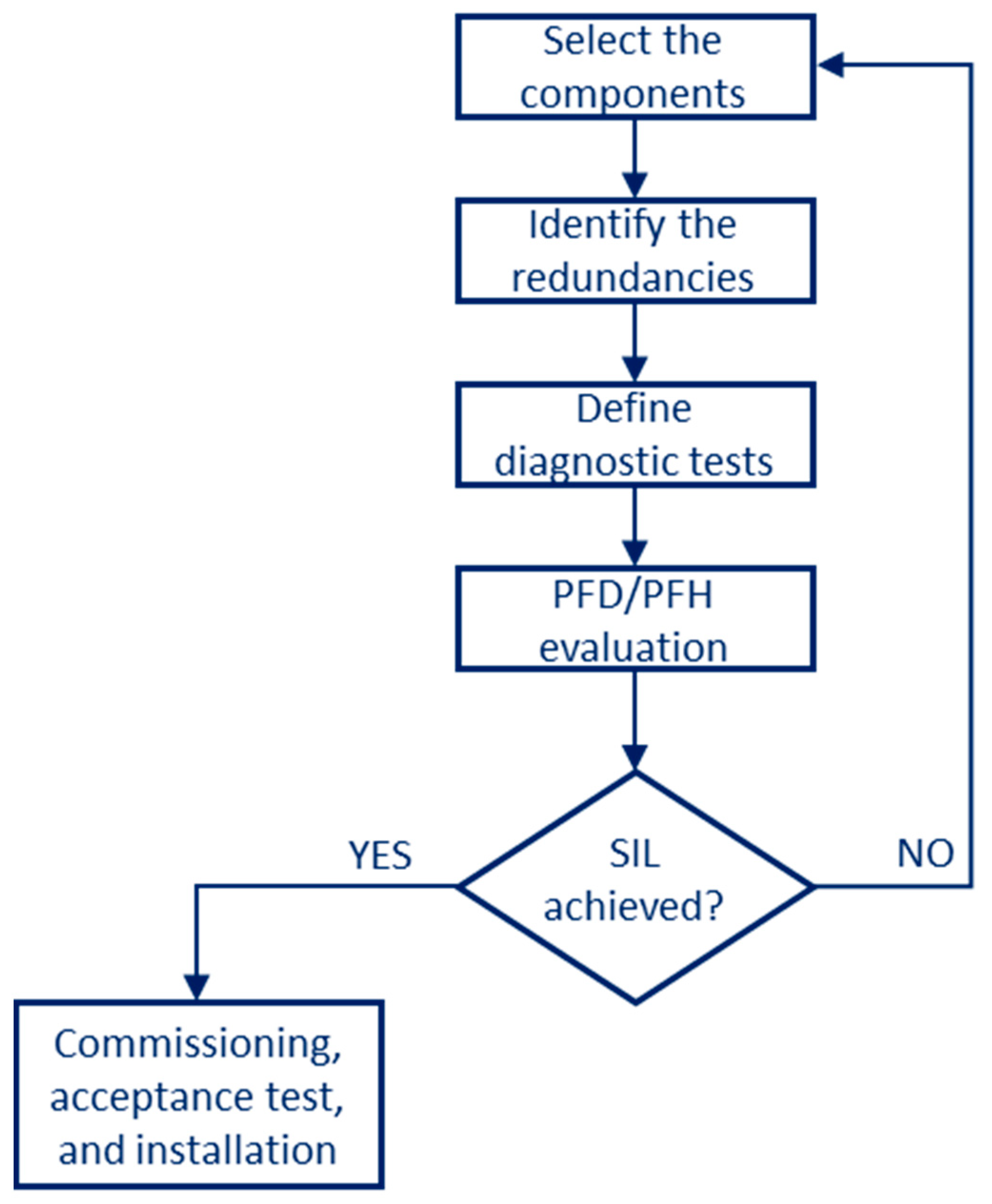
In compliance with IEC 61508:2010 [44], the SIS design is divided in several steps as illustrated in Figure 5.

The first step consists of the selection of the items making up the safety system. In order to obtain the failure rate of an element, a preliminary FMEDA (failure modes, effects, and diagnostic analysis) must be developed. After that, according to IEC61508, diagnostic coverage (DC) and safe failure fraction (SFF) are defined as follows:

$$\mathrm{DC}=\frac{{\mathsf{\lambda }}_{\mathrm{DD}}}{{\mathsf{\lambda }}_{\mathrm{DD}}+{\mathsf{\lambda }}_{\mathrm{DU}}}$$

(1)

$$\mathrm{SFF}=\frac{{\mathsf{\lambda }}_{\mathrm{SU}}+{\mathsf{\lambda }}_{\mathrm{SD}}+{\mathsf{\lambda }}_{\mathrm{DD}}}{{\mathsf{\lambda }}_{\mathrm{SU}}+{\mathsf{\lambda }}_{\mathrm{SD}}+{\mathsf{\lambda }}_{\mathrm{DU}}+{\mathsf{\lambda }}_{\mathrm{DD}}}$$

(2)

In the equations above, the failure rate of the device is divided into four different components [52,53]:

• Safe undetected failures ${\mathsf{\lambda }}_{\mathrm{SU}}$;
• Safe detected failures ${\mathsf{\lambda }}_{\mathrm{SD}}$;
• Dangerous detected failures ${\mathsf{\lambda }}_{\mathrm{DD}}$;
• Dangerous undetected failures ${\mathsf{\lambda }}_{\mathrm{DU}}$.

In other words, DC is the ratio of the probability of detected failures to the probability of all the dangerous failures and is a measure of system ability to detect failures [54,55]. Instead, SFF indicates the probability of the system failing in a safe state so it shows the percentage of possible failures that are self-identified by the device or are safe and have no effect [56,57].

In order to assess DC and SFF, the analyst has to include all the electrical, electronic, electromechanical, and mechanical items necessary to allow the system to process the required safety functions. Similarly, it is mandatory to consider all of the possible dangerous failure modes that could lead to an unsafe state, prevent a safe response on demand, or compromise the system safety integrity. Within the dangerous failures, it is necessary to estimate for each component the fraction of failures that are detected by the diagnostic tests: these tests (e.g., comparison checks in redundant architectures, additional built-in test routines, and continuous condition monitoring) are a huge contribution to the diagnostic coverage.

Architectural constraints (second step of the flowchart in Figure 5) on hardware safety integrity are a set of architectural requirements that influence the SIL assessment for each subsystem. These constraints are associated with three parameters: hardware fault tolerance, safe failure fraction, and “A/B type” classification [39,44]. Hardware fault tolerance (HFT) is the maximum number of hardware faults that will not lead to a dangerous failure. HFT of “n” means that “n + 1” faults cause a loss of a SIF. This type of fault tolerance can be increased by means of system architecture: the limit of each configuration is the number of working devices required to perform the safety function. As for all redundant architectures, common-cause failures (CCF) can nullify the redundancy. There are three different stages of hardware fault tolerance:

• HFT = 0: In a single channel architecture (1oo1), only in case of no failure the safety function can be performed.
• HFT = 1: In a dual redundancy (1oo2 or 2oo3), even in case of one failure in the sensing elements or logic solvers the safety function can still be performed.
• HFT = 2: In a triple redundancy (1oo3), up to two failures can be tolerated in order to perform the safety function.

The subsystems are classified as follows: type A units have consolidated design and the behavior in case of errors is well-known, while type B items have unknown behavior in case of failure [58]. The procedure that allows determining the optimal redundancy is called Route 1H and is shown in

Table 2. Route 1H procedure according to SIS design in compliance with IEC 61508:2010 [44]. (a) Reference values for a type A element; (b) reference values for a type B element.

(a)
SFF vs. HFT		Type A
		Hardware Fault Tolerance
		0 Faults	1 Fault	2 Faults
Safe failure fraction	<60%	SIL 1	SIL 2	SIL 3
	60–90%	SIL 2	SIL 3	SIL 4
	90–99%	SIL 3	SIL 4	SIL 4
	>99%	SIL 3	SIL 4	SIL 4
(b)
SFF vs. HFT		Type B
		Hardware Fault Tolerance
		0 Faults	1 Fault	2 Faults
Safe failure fraction	<60%	None	SIL 1	SIL 2
	60–90%	SIL 1	SIL 2	SIL 3
	90–99%	SIL 2	SIL 3	SIL 4
	>99%	SIL 3	SIL 4	SIL 4

in case of type A and type B units, respectively.

The following step requires obtaining the average probability of failure on demand varying the possible diagnostic test for each possible redundancy. There are two main categories of tests: proof tests and diagnostic tests. A proof test is a periodic test performed to detect dangerous hidden failures in a SIS [59]. In other words, a proof test is a form of a stress test with the aim of demonstrating the fitness of equipment.

Usually, it is performed on a single unit, and the structure is subjected to loads above that expected in actual use, demonstrating the safety and design margin. Anyway, a proof test is nominally a nondestructive test if both design margins and test levels are well-chosen. The frequency of conducting these tests influences the component’s average probability of failure on demand ($PF{D}_{avg}$). As a matter of fact, a higher test frequency means a lower $PF{D}_{avg}$ and a higher RRF. The PFD increases over time but returns to its original level when a proof test is performed to prove that everything works as expected. Running the same proof test twice as often lowers the average PFD. This strategy allows design engineers to meet higher SIL requirements using the same equipment or, alternatively, choosing cheaper items to achieve the same SIL target. A diagnostic test, instead, is performed periodically to detect some of the dangerous faults that prevent the SIS from responding to a demand. Some SIS may conduct self-diagnostic testing during operation in order to detect some dangerous failures immediately when they occur (essentially, a diagnostic test is a partial proof test). In order to double the full proof test interval and maintain the same average PFD, a possible approach is to run partial tests frequently [59,60]. This concept is clearly illustrated in Figure 6a, where the PFD trend in time considers only proof test procedures. On the contrary, Figure 6b shows the results of combining full proof tests and partial stroke tests (i.e., diagnostic tests).

Finally, when assessing the probability of failure on demand (PFD) of a designed SIS by means of DC and SFF, it is important to take into account uncertainties of failure rate data. The risk analysis of industrial systems and the design of a SIS are phases characterized by a remarkable level of uncertainty due to incomplete and vague information and/or insufficient knowledge and experience of the team. Some approaches available in the literature tried to deal with this problem introducing fuzzy logic, Monte Carlo simulations, sensitivity analysis, etc. (for more information, see, for instance, [58,61,62,63]).

4. Case Study: Application in the Oil and Gas Industry

This section deals with the design of a SIS for oil and gas applications in the low-demand mode of operation with the 1-year proof test interval ($T_1$ = 1 year = 8760 h). The objective of the design is to achieve the SIL 3 target because of the criticality and dangerousness of the field of application. The monitored parameter to keep the plant under control is temperature; the collected data are elaborated by a PLC and the outcomes are implemented by a pressure valve. The controller communicates with the other equipment of the SIS by using the 4–20 mA HART^® communication protocol and is able to detect under- and over-range currents, so both fail-low and fail-high conditions are detectable.

The average probability of failure on demand of a safety function for the E/E/PE safety-related system is determined by calculating and combining the average probability of failure on demand for all the subsystems which together implement the safety function; therefore, the average PFD can be expressed as follows:

$${\mathrm{PFD}}_{\mathrm{SYS}}={\mathrm{PFD}}_{\mathrm{SE}}+{\mathrm{PFD}}_{\mathrm{LS}}+{\mathrm{PFD}}_{\mathrm{FE}}$$

(3)

where the subscript SE stands for sensing element, LS is the acronym of logic solver, while FE represents the final element. The sensor stage is composed of a Rosemount^® 3144P HART^® Temperature Indicator Transmitter (TIT), a temperature monitoring device widely used at oil and gas plants. This equipment is a temperature sensor assembly made of two main parts:

• A temperature-sensing device, such as an RTD (i.e., a resistance temperature detector) or a thermocouple.
• A dedicated transmitter to communicate with the logic solver with the 4–20 mA HART^® Communication Protocol.

The TIT used is equipped with an RTD as the sensing device with the failsafe state set as fail-low; that means it is programmed to focus on low outcomes when detecting a failure: this condition is called an under-range failsafe state. The failure rates (expressed in failures in time (FIT), i.e., failures over 1 billion hours), the DC, and the SFF achieved with Equations (1) and (2) for the 3144P TIT are reported in

Table 3. Failure rates, DC (diagnostic coverage) and SFF (safe failure fraction) for the temperature sensor under analysis.

${\mathsf{\lambda }}_{\mathbf{SD}}$	${\mathsf{\lambda }}_{\mathbf{SU}}$	${\mathsf{\lambda }}_{\mathbf{DD}}$	${\mathsf{\lambda }}_{\mathbf{DU}}$	DC	SFF
2275 FIT	109 FIT	28 FIT	83 FIT	25.23%	96.67%

.

The failure rates of the sensors selected for the SIS under analysis play a fundamental role in the achievement of the specific requirements. More in detail, the higher the SIL requirement, the lower the probability of failure of the SIS must be, leading to a lower threshold of the acceptable failure rate.

Considering the SIL 3 objective for the developed SIS, the optimal redundancy for this sensor (type B element) is determined by using the procedure illustrated in Table 2 and the SFF value obtained in Table 3. Considering the abovementioned data, the optimal hardware fault tolerance for the temperature sensor under analysis is HFT = 1. Following the information reported on the 3144P TIT datasheet, the best architecture with HFT = 1 is the 2-out-of-3 (2oo3), which is made by three identical blocks connected in a parallel configuration. The three outputs are subject to a major voting mechanism: the SIF is required when at least two blocks demand it and the system state is not changed if only one channel gives a different result which disagrees with the other two channels. The employment of a redundant architecture provides some benefits in terms of system reliability and risk related to hazardous fault. The main drawback of redundancy is the issue of common-cause failures. Standard IEC 61508 [44] illustrates a procedure to evaluate two parameters $\mathsf{\beta }$ and ${\mathsf{\beta }}_{\mathrm{D}}$ that consider the effect of common-cause failures. In particular, for the considered sensor, the results are as follows: $\mathsf{\beta }=10\%$ and ${\mathsf{\beta }}_{\mathrm{D}}=5\%$. In compliance with IEC61508, considering the mean time to repair and the mean restoration time MTTR = MRT = 8 h, the average PFD for the sensor stage in the 2oo3 TIT architecture is as follows:

$$\begin{array}{c}{\mathrm{PFD}}_{\mathrm{SE}}=6{\left(\left(1-{\mathsf{\beta }}_{\mathrm{D}}\right){\mathsf{\lambda }}_{\mathrm{DD}}+\left(1-\mathsf{\beta }\right){\mathsf{\lambda }}_{\mathrm{DU}}\right)}^2{\mathrm{t}}_{\mathrm{ce}}{\mathrm{t}}_{\mathrm{ge}}+{\mathsf{\beta }}_{\mathrm{D}}{\mathsf{\lambda }}_{\mathrm{DD}}\mathrm{MTTR}\\ +\mathsf{\beta }{\mathsf{\lambda }}_{\mathrm{DU}}\left(\frac{{\mathrm{T}}_1}{2}+\mathrm{MRT}\right)\end{array}$$

(4)

where the channel equivalent mean downtime ${\mathrm{t}}_{\mathrm{ce}}$ and the system equivalent downtime ${\mathrm{t}}_{\mathrm{ge}}$ are determined using the following equations:

$${\mathrm{t}}_{\mathrm{ce}}=\frac{{\mathsf{\lambda }}_{\mathrm{DU}}}{{\mathsf{\lambda }}_{\mathrm{DU}}+{\mathsf{\lambda }}_{\mathrm{DD}}}\left(\frac{{\mathrm{T}}_1}{2}+\mathrm{MRT}\right)+\frac{{\mathsf{\lambda }}_{\mathrm{DD}}}{{\mathsf{\lambda }}_{\mathrm{DU}}+{\mathsf{\lambda }}_{\mathrm{DD}}}\mathrm{MTTR}=3.28\times {10}^3\mathrm{h}$$

(5)

$${\mathrm{t}}_{\mathrm{ge}}=\frac{{\mathsf{\lambda }}_{\mathrm{DU}}}{{\mathsf{\lambda }}_{\mathrm{DU}}+{\mathsf{\lambda }}_{\mathrm{DD}}}\left(\frac{{\mathrm{T}}_1}{3}+\mathrm{MRT}\right)+\frac{{\mathsf{\lambda }}_{\mathrm{DD}}}{{\mathsf{\lambda }}_{\mathrm{DU}}+{\mathsf{\lambda }}_{\mathrm{DD}}}\mathrm{MTTR}=2.19\times {10}^3\mathrm{h}$$

(6)

Considering Equations (4)–(6) and substituting the values above, the probability of failure on demand of the sensing element ${\mathrm{PFD}}_{\mathrm{SE}}$ is:

$${\mathrm{PFD}}_{\mathrm{SE}}=3.68\times {10}^{-5}$$

(7)

A Moore Industries^® Safety Trip Alarm (STA) logic solver is used as the second block of the SIS chain. This controller is used to:

• Provide emergency shutdown.
• Warn of unwanted process conditions.
• Provide on/off control in both SIS and traditional alarm trip applications.

The failure rates, the DC, and the SFF achieved with Equations (1) and (2) for the STA logic solver under analysis are reported in

Table 4. Failure rates, DC (diagnostic coverage), and SFF (safe failure fraction) for the logic solver under analysis.

${\mathsf{\lambda }}_{\mathbf{SD}}$	${\mathsf{\lambda }}_{\mathbf{SU}}$	${\mathsf{\lambda }}_{\mathbf{DD}}$	${\mathsf{\lambda }}_{\mathbf{DU}}$	DC	SFF
0 FIT	660 FIT	170 FIT	86 FIT	66.41%	90.61%

.

According to SIL 3 objective for the SIS, the optimal redundancy for this sensor (type B element) is HFT = 1. In compliance with the sensor stage, the configuration that best fits this condition is the 2oo3, so that each TIT is connected with one STA. Redundancy in the logic solver leads to common-cause failures and the parameters to evaluate them are $\mathsf{\beta }=10\%$ and ${\mathsf{\beta }}_{\mathrm{D}}=10\%$. Considering MTTR = MRT = 8 h and taking into account the 2oo3 architecture, the PFD of the logic solver is as follows:

$${\mathrm{PFD}}_{\mathrm{LS}}=6{\left(\left(1-{\mathsf{\beta }}_{\mathrm{D}}\right){\mathsf{\lambda }}_{\mathrm{DD}}+\left(1-\mathsf{\beta }\right){\mathsf{\lambda }}_{\mathrm{DU}}\right)}^2{\mathrm{t}}_{\mathrm{ce}}{\mathrm{t}}_{\mathrm{ge}}+{\mathsf{\beta }}_{\mathrm{D}}{\mathsf{\lambda }}_{\mathrm{DD}}\mathrm{MTTR}+\mathsf{\beta }{\mathsf{\lambda }}_{\mathrm{DU}}\left(\frac{{\mathrm{T}}_1}{2}+\mathrm{MRT}\right)$$

(8)

$${\mathrm{t}}_{\mathrm{ce}}=\frac{{\mathsf{\lambda }}_{\mathrm{DU}}}{{\mathsf{\lambda }}_{\mathrm{DU}}+{\mathsf{\lambda }}_{\mathrm{DD}}}\left(\frac{{\mathrm{T}}_1}{2}+\mathrm{MRT}\right)+\frac{{\mathsf{\lambda }}_{\mathrm{DD}}}{{\mathsf{\lambda }}_{\mathrm{DU}}+{\mathsf{\lambda }}_{\mathrm{DD}}}\mathrm{MTTR}=1.47\times {10}^3\mathrm{h}$$

(9)

$${\mathrm{t}}_{\mathrm{ge}}=\frac{{\mathsf{\lambda }}_{\mathrm{DU}}}{{\mathsf{\lambda }}_{\mathrm{DU}}+{\mathsf{\lambda }}_{\mathrm{DD}}}\left(\frac{{\mathrm{T}}_1}{3}+\mathrm{MRT}\right)+\frac{{\mathsf{\lambda }}_{\mathrm{DD}}}{{\mathsf{\lambda }}_{\mathrm{DU}}+{\mathsf{\lambda }}_{\mathrm{DD}}}\mathrm{MTTR}=989\mathrm{h}$$

(10)

$${\mathrm{PFD}}_{\mathrm{LS}}=3.83\times {10}^{-5}$$

(11)

A redundant control system (RCS) by ASCO^® is the final element selected for this application. It is an electromechanical and pneumatic system consisting of two solenoid valves and one pneumatic valve (bypass valve). In order to screen the pressures at dangerous points of the RCS, the actuator is provided by three pressure switches on each valve for diagnostic purposes. The switch contacts are closed in the presence of pressure because they are normally open.

According to the international standard IEC 6150 [44], the RCS is utilized as the final element of the SIS together with a controlled block valve (BV). In particular, in this design, the RCS is considered in series with an X Series Ball Valve with the floating ball design. The objective is to move toward the safe state in brief time. The safe state is obtained with de-energized signals so at least one of the two solenoid valves has to be energized to prevent the block valve from moving to the safe state. The failure rates for the RCS are reported in

Table 5. Failure rate of the RCS equipment composed of a solenoid valve, a bypass valve, and a pressure switch.

Device	${\mathsf{\lambda }}_{\mathbf{SD}}$	${\mathsf{\lambda }}_{\mathbf{SU}}$	${\mathsf{\lambda }}_{\mathbf{DD}}$	${\mathsf{\lambda }}_{\mathbf{DU}}$
Solenoid valve	594 FIT	216 FIT	502 FIT	10 FIT
Bypass valve	57 FIT	88 FIT	7 FIT	0 FIT
Pressure switch	444 FIT	5 FIT	0 FIT	0 FIT
Complete RCS	1095 FIT	309 FIT	507 FIT	10 FIT

.

The safe failure fraction of the final element can be calculated using Equation (2) and the failure rate data included in Table 5. The obtained value is SFF = 99.38%. Consequently, through Table 2 for type A element, the required redundancy to achieve the SIL 3 target is HFT = 0.

In particular, the selected configuration is a single RCS element in a specific safety mode of operation called where only one solenoid valve is online in the standard work condition. The logic solver can detect every spurious trip of this operative valve by using the relative pressure switch outcome. In order to preserve air supply to the ball valve, the control unit energizes the other solenoid valve when a spurious trip is revealed.

Using a Markov diagram, it is possible to model the behavior of the component in various states using a memoryless process in which the next state of the item is only dependent on the transition values and the current state of the system [64,65]. Considering MTTR = 24 h and taking into account the Markov diagram suggested by the standard IEC 61508:2010 [44], then the average probability of failures on demand for RCS is:

$$PF{D}_{F{E}_{RCS}}=1.24\times {10}^{-4}$$

(12)

In order to monitor the dangerous failures of the utilized block valve (undetected by the standard diagnostics), a partial valve stroke test (PVST) is provided. The latter is a delicate procedure in particular in high energy and high flow applications where it could generate a response (and instabilities) in the process control system or in the safety instrumented system leading to a spurious trip.

The average PFD assessment follows a different procedure when a PVST is applied. Considering the failure rates in

Table 6. Failure rates of the block valve included in the final element.

${\mathsf{\lambda }}_{\mathbf{SD}}$	${\mathsf{\lambda }}_{\mathbf{SU}}$	${\mathsf{\lambda }}_{\mathbf{DD}}$	${\mathsf{\lambda }}_{\mathbf{DU}}$
0 FIT	0 FIT	149 FIT	330 FIT

and MTTR = 96 h, according to the international standard IEC 61508 and using Markov diagrams, the average PFD of the block valve is:

$$PF{D}_{F{E}_{BV}}=5.05\times {10}^{-4}$$

(13)

Thus, the average PFD of the final element stage assembly by the RCS and the block valve is as follows:

$$\begin{array}{c}PF{D}_{FE}=PF{D}_{F{E}_{RCS}}+PF{D}_{F{E}_{BV}}=1.24\times {10}^{-4}+5.05\times {10}^{-4}\\ =6.29\times {10}^{-4}\end{array}$$

(14)

The average probability of failure on demand $PF{D}_{avg}$ associated to a single safety function SIF of the developed SIS is obtained by summing the single PFD of all the subsystems (sensor stage, logic solver stage, final element stage) involved in the SIF. According to Equation (3), the probability of failure on demand of the whole system is as follows:

$$PF{D}_{SYS}=3.68\times {10}^{-5}+3.83\times {10}^{-5}+6.29\times {10}^{-4}=7\times 04\times {10}^{-4}$$

(15)

A summary of the developed SIS is included in

Table 7. Summary of the developed SIS.

Element	Model	Manufacturer	Capability	Selected Configuration	Calculated Average PFD
Sensing element	3144P Temperature Transmitter equipped with RTD	Rosemount	SIL 3 capable	2oo3	3.68 × 10−5
Logic solver	STA Programmable Safety Trip Alarm	Moore Industries	SIL 3 capable	2oo3	3.83 × 10−5
Final element	Redundant Control System	ASCO	SIL 3 capable	1oo1	1.24 × 10−4
Final element	X Series Ball Valve	ABC Valve	SIL 3 capable	1oo1	5.05 × 10−4

, focusing on the product detail of each specific component selected in this work.

In compliance with the translation table between the SIL target and the average PFD described in IEC 61508 [44], for the SIS under test, the SIL 3 objective is reached because the average probability of failure on demand of the whole SIS belongs to the range of SIL3 attribution, as highlighted in

Table 8. SIL and the corresponding PFD and PFH targets.

SIL	Low-Demand Mode of Operation PFDavg	High-Demand Mode of Operation PFH (h−1)
4	≥10−5 to <10−4	≥10−9 to <10−8
3	≥10−4 to <10−3	≥10−8 to <10−7
2	≥10−3 to <10−2	≥10−7 to <10−6
1	≥10−2 to <10−1	≥10−6 to <10−5

.

Figure 7 shows a pie chart of each contribution of the whole probability of failure on demand, highlighting that the greatest share refers to the final element, about 18% to the whole RCS system, and 72% to the block valve with a consequent whole percentage of 90%. The sensor and the logic solver are characterized by a small value of PFD, therefore, each one gives a 5% contribution to the whole PFD.

According to the literature (see, for instance, [37,38,44,47]), a realistic partition of the average system PFD widely accepted is 35% to the sensor stage, 15% to the logic solver stage, and 50% to the final element stage. In this application, the actuator is composed of a chain of two complex valves in the 1oo1 architecture, thus this configuration leads to associate 90% of the whole PFD to the final stage.

Figure 8 shows the average PFD assessed to the sensor stage (blue columns), to the logic solver stage (red columns), and to the final element stage (orange columns) considering a 1-year, 2-year, and 3-year proof test interval.

The figure highlights that at a higher value of PFD calculated with a 1-year proof test interval, the proof test interval increase corresponds with greater PFD increases. Instead, the PFD assessed to the least critical subsystem (a sensor and a logic solver) is characterized by a little increase when the proof test interval increases.

5. Conclusions

This paper deals with a diagnostics-oriented approach for the design of safety instrumented systems at oil and gas plants.

After an accurate review of diagnostic strategies to successfully implement condition monitoring at industrial plants, the design of an actual SIS is presented paying great attention to the role of diagnostics. The considered SIS is used in the oil and gas application, and it is composed of a sensor stage in the 2oo3 configuration, three logic solvers (one for each sensor) capable to elaborate data and activate the safety function, and a final element composed of an RCS system and a block valve in the series configuration. The paper emphasizes the need in a limit alarm trip, on-board diagnostics, and logic solver diagnostics to achieve low probability of failure on demand and ensure high SIL levels.

Redundant architectures improve system reliability and availability, decreasing the probability of dangerous failures. However, additional components require taking into account properly all common-cause failures during the design phase. The proposed diagnostics-oriented solution for safety improvements follows these steps: improve common cause strength, use diversity, use online condition monitoring and diagnostics, and add redundancy. Clearly, each choice is a tradeoff between safety and costs: to take these decisions, designers should select the best safety improvement, taking into account not only data provided by suppliers (usually validated in a laboratory environment), but considering real-world installed safety (which is always much worse). Only by quantifying installed safety designers can evaluate the real-world safety and cost impact of specific technology. The case study highlights these steps emphasizing the critical role of valves and redundant control systems accounting for 90% of the probability of failure on demand. This research is intended to be used as a guidance for the further design of safety instrumented systems in the oil and gas industry. Further study should focus on how to improve diagnostic, prognostic, and health monitoring and valves and actuators for oil and gas safety-related systems in order to reduce the probability of failure on demand of these critical items.

References

- Ciani, L.; Bartolini, A.; Guidi, G.; Patrizi, G. A hybrid tree sensor network for a condition monitoring system to optimise maintenance policy. Acta IMEKO 2020, 9, 3–9. [Google Scholar] [CrossRef]
- D’Emilia, G.; Natale, E. Network of MEMS sensors for condition monitoring of industrial systems: Accuracy assessment of features used for diagnosis. In Proceedings of the 17th IMEKO TC 10 and EUROLAB Virtual Conference “Global Trends in Testing, Diagnostics & Inspection for 2030”and EUROLAB Virtual Conference “Global Trends in Testing, Diagnostics and Inspection for 2030”, Virtual, 20–22 October 2020; pp. 356–361. [Google Scholar]
- D’Emilia, G.; Gaspari, A.; Natale, E. Sensor fusion for more accurate features in condition monitoring of mechatronic systems. In Proceedings of the 2019 IEEE International Instrumentation and Measurement Technology Conference (I2MTC), Auckland, New Zealand, 20–23 May 2019; pp. 1–6. [Google Scholar]
- Ciani, L.; Bartolini, A.; Guidi, G.; Patrizi, G. Condition Monitoring of Wind Farm based on Wireless Mesh Network. In Proceedings of the 16th IMEKO TC10 Conference: “Testing, Diagnostics & Inspection as a Comprehensive Value Chain for Quality & Safety”, Berlin, Germany, 3–4 September 2019; pp. 39–44. [Google Scholar]
- Kulwanoski, G.; Gaynes, M.; Smith, A.; Darrow, B. Electrical contact failure mechanisms relevant to electronic packages. In Proceedings of the Electrical Contacts—1991 Thirty-Seventh IEEE HOLM Conference on Electrical Contacts, Chicago, IL, USA, 6–9 October 1991; pp. 184–192. [Google Scholar]
- Catelani, M.; Ciani, L.; Venzi, M. Component Reliability Importance assessment on complex systems using Credible Improvement Potential. Microelectron. Reliab. 2016, 64, 113–119. [Google Scholar] [CrossRef]
- González-González, A.; Jimenez Cortadi, A.; Galar, D.; Ciani, L. Condition monitoring of wind turbine pitch controller: A maintenance approach. Measurement 2018, 123, 80–93. [Google Scholar] [CrossRef]
- Ciani, L.; Guidi, G.; Patrizi, G.; Galar, D. Condition-Based Maintenance of HVAC on a High-Speed Train for Fault Detection. Electronics 2021, 10, 1418. [Google Scholar] [CrossRef]
- Galar, D.; Sandborn, P.; Kumar, U. Maintenance Costs and Life Cycle Cost Analysis; CRC Press: Boca Raton, FL, USA; Taylor & Francis Group: Abingdon, UK, 2017; ISBN 9781498769549. [Google Scholar]
- Ciani, L.; Guidi, G.; Patrizi, G.; Venzi, M. System Maintainability Improvement using Allocation Procedures. In Proceedings of the 2018 IEEE International Systems Engineering Symposium (ISSE), Rome, Italy, 1–3 October 2018; pp. 1–6. [Google Scholar]
- Capriglione, D.; Carratu, M.; Pietrosanto, A.; Sommella, P. Online Fault Detection of Rear Stroke Suspension Sensor in Motorcycle. IEEE Trans. Instrum. Meas. 2019, 68, 1362–1372. [Google Scholar] [CrossRef]
- Kumar, U.; Galar, D.; Parida, A.; Stenström, C.; Berges, L. Maintenance performance metrics: A state-of-the-art review. J. Qual. Maint. Eng. 2013, 19, 233–277. [Google Scholar] [CrossRef] [Green Version]
- Frosini, L. Novel Diagnostic Techniques for Rotating Electrical Machines—A Review. Energies 2020, 13, 5066. [Google Scholar] [CrossRef]
- Martin, K.F. A review by discussion of condition monitoring and fault diagnosis in machine tools. Int. J. Mach. Tools Manuf. 1994, 34, 527–551. [Google Scholar] [CrossRef]
- Ugwiri, M.A.; Carratu, M.; Pietrosanto, A.; Paciello, V.; Lay-Ekuakille, A. Vibrations Measurement and Current Signatures for Fault Detection in Asynchronous Motor. In Proceedings of the 2020 IEEE International Instrumentation and Measurement Technology Conference (I2MTC), Dubrovnik, Croatia, 25–28 May 2020; pp. 1–6. [Google Scholar]
- Capriglione, D.; Carratu, M.; Pietrosanto, A.; Sommella, P. Soft Sensors for Instrument Fault Accommodation in Semiactive Motorcycle Suspension Systems. IEEE Trans. Instrum. Meas. 2020, 69, 2367–2376. [Google Scholar] [CrossRef]
- Aizenberg, I.; Corti, F.; Grasso, F.; Luchetta, A.; Manetti, S.; Piccirilli, M.C.; Reatti, A.; Kazimierczuk, M.K. A multi-step approach to the single fault diagnosis of DC-DC switched power converters. In Proceedings of the 2018 IEEE International Symposium on Circuits and Systems (ISCAS), Florence, Italy, 27–30 May 2018; pp. 1–5. [Google Scholar]
- Petkov, N.; Wu, H.; Powell, R. Cost-benefit analysis of condition monitoring on DEMO remote maintenance system. Fusion Eng. Des. 2020, 160, 112022. [Google Scholar] [CrossRef]
- Dhillon, B.S. Safety and Reliability in the Oil and Gas Industry; CRC Press: Boca Raton, FL, USA, 2016; ISBN 9780429183713. [Google Scholar]
- Center for Chemical Process Safety of the American Institute of Chemical Engineers. Process Safety in Upstream Oil and Gas; John Wiley & Sons, Inc.: Hoboken, NJ, USA, 2021; ISBN 9781119620044. [Google Scholar]
- Loboda, I. Gas Turbine Diagnostics. In Efficiency, Performance and Robustness of Gas Turbines; InTech: Rijeka, Croatia, 2012. [Google Scholar]
- Timms, C. Hazards equal trips or alarms or both. Process Saf. Environ. Prot. 2009, 87, 3–13. [Google Scholar] [CrossRef]
- Catelani, M.; Ciani, L.; Guidi, G.; Patrizi, G. Reliability Analysis of diagnostic system for Condition Monitoring of industrial plant. In Proceedings of the 2021 IEEE 6th International Forum on Research and Technology for Society and Industry (RTSI), Naples, Italy, 6–9 September 2021; pp. 323–328. [Google Scholar]
- Wei, L.; Duan, H.; Jia, D.; Jin, Y.; Chen, S.; Liu, L.; Liu, J.; Sun, X.; Li, J. Motor oil condition evaluation based on on-board diagnostic system. Friction 2020, 8, 95–106. [Google Scholar] [CrossRef] [Green Version]
- Saibannavar, D.; Math, M.M.; Kulkarni, U. A Survey on On-Board Diagnostic in Vehicles. In International Conference on Mobile Computing and Sustainable Informatics; Springer: Cham, Switzerland, 2020; pp. 49–60. [Google Scholar]
- Isermann, R. Mechatronic Systems. Fundamentals; Springer: Berlin/Heidelberg, Germany, 2005. [Google Scholar]
- Li, Y.; Wang, Y.; Ma, C. Design of communication system in intelligent instrument based on HART protocol. In Proceedings of the 2015 IEEE International Conference on Mechatronics and Automation (ICMA), Beijing, China, 2–5 August 2015; pp. 351–356. [Google Scholar]
- Micallef, C.J.; Ostling, C.H.; Parks, C. Apparatus and Method to Power 2-Wire Field Devices, Including HART, Foundation Fieldbus, and Profibus PA, for Configuration 2013. U.S. Patent 8,344,542, 1 January 2013. [Google Scholar]
- Pongswatd, S.; Julsereewong, A.; Thepmanee, T. Combined HART- FFH1 Solution Using IEC 61804 for PID Control in Revamp Projects. In Proceedings of the 2018 International Conference on Engineering, Applied Sciences, and Technology (ICEAST), Phuket, Thailand, 4–7 July 2018; pp. 1–4. [Google Scholar]
- Grimmelius, H.T.; Meiler, P.P.; Maas, H.L.M.M.; Bonnier, B.; Grevink, J.S.; van Kuilenburg, R.F. Three state-of-the-art methods for condition monitoring. IEEE Trans. Ind. Electron. 1999, 46, 407–416. [Google Scholar] [CrossRef] [Green Version]
- Hong, S.H.; Song, S.M. Transmission of a Scheduled Message Using a Foundation Fieldbus Protocol. IEEE Trans. Instrum. Meas. 2008, 57, 268–275. [Google Scholar] [CrossRef]
- Soares, C. Gas Turbines. A Handbook of Air, Land and Sea Applications; Elsevier: Amsterdam, The Netherlands, 2015; ISBN 9780124104617. [Google Scholar]
- Catelani, M.; Ciani, L.; Venzi, M. Failure Modes and Mechanisms of Sensors Used in Oil&Gas Applications. In Proceedings of the Lecture Notes in Electrical Engineering, 4th National Conference on Sensors; Springer: Cham, Switzerland, 2019; pp. 429–436. [Google Scholar]
- Liu, Y.; Rausand, M. Proof-testing strategies induced by dangerous detected failures of safety-instrumented systems. Reliab. Eng. Syst. Saf. 2016, 145, 366–372. [Google Scholar] [CrossRef] [Green Version]
- Goble, W.M.; Brombacher, A.C. Using a failure modes, effects and diagnostic analysis (FMEDA) to measure diagnostic coverage in programmable electronic systems. Reliab. Eng. Syst. Saf. 1999, 66, 145–148. [Google Scholar] [CrossRef] [Green Version]
- Wacker, H.D.; Holub, P.; Borcsok, J. Optimization of diagnostics with respect to the diagnostic coverage and the cost function. In Proceedings of the 2013 XXIV International Conference on Information, Communication and Automation Technologies (ICAT), Sarajevo, Bosnia and Herzegovina, 30 October–1 November 2013; pp. 1–7. [Google Scholar]
- Catelani, M.; Ciani, L.; Luongo, V. Safety analysis in oil & gas industry in compliance with standards IEC61508 and IEC61511: Methods and applications. In Proceedings of the 2013 IEEE International Instrumentation and Measurement Technology Conference (I2MTC), Minneapolis, MN, USA, 6–9 May 2013; pp. 686–690. [Google Scholar]
- Catelani, M.; Ciani, L.; Mugnaini, M.; Scarano, V.; Singuaroli, R. Definition of Safety Levels and Performances of Safety: Applications for an Electronic Equipment Used on Rolling Stock. In Proceedings of the 2007 IEEE Instrumentation & Measurement Technology Conference IMTC 2007, Warsaw, Poland, 1–3 May 2007; pp. 1–4. [Google Scholar]
- Selvik, J.T.; Signoret, J.-P. How to interpret safety critical failures in risk and reliability assessments. Reliab. Eng. Syst. Saf. 2017, 161, 61–68. [Google Scholar] [CrossRef]
- Ciani, L.; Guidi, G.; Patrizi, G. Condition-based Maintenance for Oil&Gas system basing on Failure Modes and Effects Analysis. In Proceedings of the 2019 IEEE 5th International forum on Research and Technology for Society and Industry (RTSI), Florence, Italy, 9–12 September 2019; pp. 85–90. [Google Scholar]
- Catelani, M.; Ciani, L.; Guidi, G.; Patrizi, G. An enhanced SHERPA (E-SHERPA) method for human reliability analysis in railway engineering. Reliab. Eng. Syst. Saf. 2021, 215, 107866. [Google Scholar] [CrossRef]
- Capriglione, D.; Carratu, M.; Pietrosanto, A.; Sommella, P.; Catelani, M.; Ciani, L.; Patrizi, G.; Singuaroli, R.; Signorini, L. Characterization of Inertial Measurement Units under Environmental Stress Screening. In Proceedings of the 2020 IEEE International Instrumentation and Measurement Technology Conference (I2MTC), Dubrovnik, Croatia, 25–28 May 2020; pp. 1–6. [Google Scholar]
- Stapelberg, R.F. Handbook of Reliability, Availability, Maintainability and Safety in Engineering Design; Springer: London, UK, 2009; ISBN 978-1-84800-174-9. [Google Scholar]
- IEC 61508; Functional Safety of Electrical/Electronic/Programmable Electronic Safety-Related Systems. Part 1–7. International Electrotechnical Commission: Geneva, Switzerland, 2010.
- Hayek, A.; Borcsok, J. Safety chips in light of the standard IEC 61508: Survey and analysis. In Proceedings of the 2014 International Symposium on Fundamentals of Electrical Engineering (ISFEE), Bucharest, Romania, 28–29 November 2014; pp. 1–6. [Google Scholar]
- Torres, E.S.; Sriramula, S.; Celeita, D.; Ramos, G. Model for Assessing the Safety Integrity Level of Electrical/ Electronic/Programmable Electronic Safety-Related Systems. In Proceedings of the 2019 IEEE Industry Applications Society Annual Meeting, Baltimore, MD, USA, 29 September–3 October 2019; pp. 1–7. [Google Scholar]
- Rausand, M. Reliability of Safety-Critical Systems; John Wiley & Sons, Inc.: Hoboken, NJ, USA, 2014; ISBN 9781118112724. [Google Scholar]
- Maurya, A.; Kumar, D. Reliability of safety-critical systems: A state-of-the-art review. Qual. Reliab. Eng. Int. 2020, 36, 2547–2568. [Google Scholar] [CrossRef]
- Theophilus, S.C.; Esenowo, V.N.; Arewa, A.O.; Ifelebuegu, A.O.; Nnadi, E.O.; Mbanaso, F.U. Human factors analysis and classification system for the oil and gas industry (HFACS-OGI). Reliab. Eng. Syst. Saf. 2017, 167, 168–176. [Google Scholar] [CrossRef]
- Kukfisz, B.; Kuczyńska, A.; Piec, R.; Szykuła-Piec, B. Research on the Safety and Security Distance of Above-Ground Liquefied Gas Storage Tanks and Dispensers. Int. J. Environ. Res. Public Health 2022, 19, 839. [Google Scholar] [CrossRef]
- Ciani, L.; Guidi, G.; Patrizi, G.; Galar, D. Improving Human Reliability Analysis for Railway Systems Using Fuzzy Logic. IEEE Access 2021, 9, 128648–128662. [Google Scholar] [CrossRef]
- Shin, H.K.; Oh, J.-S.; Suh, J.-H.; Jo, S.-M.; Yu, M.-H.; Song, I. Design evaluation of hardwired F-LIC module for ITER AC/DC converters by FMEDA method. Fusion Eng. Des. 2020, 151, 111417. [Google Scholar] [CrossRef]
- Kim, S.K.; Kim, Y.S. An evaluation approach using a HARA and FMEDA for the hardware SIL. J. Loss Prev. Process Ind. 2013, 26, 1212–1220. [Google Scholar] [CrossRef]
- Granig, W.; Hammerschmidt, D.; Zangl, H. Diagnostic coverage estimation method for optimization of redundant sensor systems. In Proceedings of the 2017 IEEE SENSORS, Glasgow, UK, 29 October–1 November 2017; pp. 1–3. [Google Scholar]
- Yeon, K.; Lee, D. Fault detection and diagnostic coverage for the domain control units of vehicle E/E systems on functional safety. In Proceedings of the 2017 20th International Conference on Electrical Machines and Systems (ICEMS), Sydney, NSW, Australia, 11–14 August 2017; pp. 1–4. [Google Scholar]
- Yoshimura, I.; Sato, Y. Safety Achieved by the Safe Failure Fraction (SFF) in IEC 61508. IEEE Trans. Reliab. 2008, 57, 662–669. [Google Scholar] [CrossRef]
- Smith, D.; Simpson, K. Assessing Safe Failure Fraction and Diagnostic Coverage. In The Safety Critical Systems Handbook; Elsevier: Amsterdam, The Netherlands, 2016; pp. 303–305. [Google Scholar]
- Piesik, E.; Śliwiński, M.; Barnert, T. Determining and verifying the safety integrity level of the safety instrumented systems with the uncertainty and security aspects. Reliab. Eng. Syst. Saf. 2016, 152, 259–272. [Google Scholar] [CrossRef]
- ISO 14224:2006; Petroleum, Petrochemical and Natural Gas Industries—Collection and Exchange of Reliability and Maintenance Data for Equipment. International Organization for Standardization: Geneva, Switzerland, 2016.
- Lundteigen, M.A.; Rausand, M. The effect of partial stroke testing on the reliability of safety valves. In Proceedings of the European Safety and Reliability Conference 2007 (ESREL 2007), Stavanger, Norway, 25–27 June 2007; pp. 2479–2486. [Google Scholar]
- Markowski, A.S.; Siuta, D. Fuzzy logic approach for identifying representative accident scenarios. J. Loss Prev. Process Ind. 2018, 56, 414–423. [Google Scholar] [CrossRef]
- Markowski, A.S.; Siuta, D. Selection of representative accident scenarios for major industrial accidents. Process Saf. Environ. Prot. 2017, 111, 652–662. [Google Scholar] [CrossRef]
- Liu, H.-C.; You, J.-X.; Li, P.; Su, Q. Failure Mode and Effect Analysis Under Uncertainty: An Integrated Multiple Criteria Decision Making Approach. IEEE Trans. Reliab. 2016, 65, 1380–1392. [Google Scholar] [CrossRef]
- Birolini, A. Reliability Engineering—Theory and Practice, 8th ed.; Springer: Berlin/Heidelberg, Germany, 2017. [Google Scholar]
- Rausand, M.; Barros, A.; Høyland, A. System Reliability Theory. Models, Statistical Methods, and Applications; John Wiley & Sons, Inc.: Hoboken, NJ, USA, 2021; ISBN 9781119373520. [Google Scholar]
Figure 1.
Example of limit alarm trip implementation considering the time behavior of a generic sensor’s output.
Figure 2.
Schematic representation of wiring connections for sensors’ on-board diagnostics: (a) 4–20 mA HART® protocol; (b) Foundation Fieldbus.
Figure 3.
Output range and safety thresholds for a 4–20 mA analog sensor in case of logic solver diagnostics.
Figure 4.
Functional block diagram of a generic safety instrumented system.
Figure 5.
Flowchart of SIS design according to IEC 61508:2010 [44].
Figure 6.
Time behavior of the probability of failure on demand for a generic SIS. (a) Only a full proof test is put in practice; (b) full proof tests and diagnostic tests are performed.
Figure 7.
Pie chart of each contribution of the probability of failure on demand. The percentages were obtained by normalizing results achieved in Equations (4)–(8).
Figure 8.
Average PFD of all the subsystems involved in the SIS vs. the proof test interval.