Exploring the Response of the Japanese Sardine (Sardinops melanostictus) Stock-Recruitment Relationship to Environmental Changes under Different Structural Models

Abstract

Japanese sardines (Sardinops melanostictus) are environmentally sensitive pelagic fish. We investigated the effects of environmental factors on the stock-recruitment (S-R) relationship of S. melanostictus in the Pacific Ocean from 1984 to 2018. We modeled and analyzed the recruitment of S. melanostictus using the Ricker model, the Ricker environment extension model (Ricker-E), and the generalized additive model (GAM). Different numbers of environmental factors were added to the models for fitting, and the Akaike information criterion (AIC) was used to select the optimal model. The results showed that the nonlinear GAM provided the best fit. The results of the GAM single factor and multifactor analysis showed that environmental factors were significantly correlated with recruitment in S. melanostictus (p < 0.05). The best fitting model was the GAM, with an AIC of 57.9 and a cumulative explanation rate of 95.7%. Sea surface temperature was the most dominant environmental factor and had a negative impact on R/S. Considering both spawning stock biomass (S) and the environmental factors in the S-R relationship is important for studying the mechanisms of complementary changes and population changes in S. melanostictus under the influence of the marine environment.

1. Introduction

Fluctuations in fishery resources have been closely associated with changes in the global climate and marine environment [1]. Small pelagic fish are not only critical species in the ecosystem, but also essential economic fish, accounting for approximately 20–25% of the global catch annually [2,3,4]. Small pelagic fish are fast-growing and short-lived, with high natural mortality, which means that changes in their recruitment influence the size of the population. Therefore, the success rate of their recruitment is an essential factor in population dynamics and development [5,6]. However, recruitment is susceptible to changes in the complex marine environment of the waters in which they inhabit, and this responds very rapidly to changes in the climate, having a high degree of population variability. Therefore, it is necessary to investigate the effects of climate change and marine environmental changes on small pelagic fish populations.

The Japanese sardine (Sardinops melanostictus) is a representative species of small pelagic migratory fish that has a significant ecological and commercial value [7,8,9]. The species is primarily distributed in the Northwest Pacific region of China, Japan, and Korea, with spawning grounds on nearly all coastlines and adjacent water [10]. Information regarding S. melanostictus has previously been reported, including biological measurements [11], spawning [12], larval reproductive development [13], and environmental factors that affect population dynamics [14]. Morimoto [15] studied the relationship between different interannual variables and the age, body length, and weight of S. melanostictus. He suggested that age and growth changes in S. melanostictus are among the factors affecting fluctuations of the population. The relationship between spawning stock and recruitment is crucial to investigate, since the environment in which fish live significantly impacts their spawning, development, and growth. Fishery stock assessment and management are based on the spawning stock-recruitment (S-R) relationship [16,17]. The population biomass of S. melanostictus has undergone dramatic fluctuations on a multidecade scale [3,18]. Wada and Jacobson [19] pointed out that the dynamics of recruitment under the influence of the environment and density are important factors in the fluctuation of the S. melanostictus population. Ganias [20] revealed the relationship between environmental factors (sea surface temperatures and chlorophyll-a) and the sardine spawning rate. Takasuka et al. [21] reported that sardines grow more slowly in warmer environments. The environmental changes experienced during spawning or migration are among the key reasons for reproductive failure. Therefore, environmental factors [22], such as the February Arctic Oscillation (AO) [23,24], the Pacific Decadal Oscillation (PDO), and the sea surface temperatures (SST), should also be considered in sardine population dynamics and complementary predictive modeling studies.

Many studies have investigated the effects of environmental factors on the S-R relationship of S. melanostictus. However, studies have focused more on the effects of a single environmental impact or a single model aspect [22,25,26]. In contrast, this study focuses on comparing multiple models with different structures under the influence of the environment, to find the best model for describing S-R relationships. To understand the recruitment of S. melanostictus, we assumed that biomass dynamics are the result of a combination of density-dependent and density-independent factors (changes in the marine environment). We developed the traditional Ricker model, Ricker environment extension model (Ricker-E), and generalized additive model (GAM), to explore the critical environmental factors of S. melanostictus biomass dynamics under different model structures. The effect of fishing is considered an important factor in the development of the population, especially in the case of low spawner levels, where fishing pressure can hinder the recovery and development of the population. Therefore, we should promptly adjust management strategies through resource assessment, to achieve the sustainable development of fishery resources. This is of great practical importance for future research on the dynamics of S. melanostictus populations, fisheries resource management, and conservation.

2. Materials and Methods

2.1. Data Source

2.1.1. Fishery Data

The area of this study was the Kuroshio-Oyashio system in Japanese waters of the Pacific Northwest. Our data were obtained from the Japan Fisheries Agency report of 2019, selecting biological data for S. melanostictus (stock spawning biomass 10² kt) and recruitment (in number/10² million ind) from 1984 to 2018. Recruitment was taken as the number of fish aged 0 [27].

2.1.2. Environmental Factors

The spawning area of S. melanostictus is located in the Kuroshio-Oyashio system (Figure 1), and the temperature in this area has a significant correlation with the density of sardines [28,29]. Changes in the marine environment in the Kuroshio-Oyashio area affect the reproductive success rate of sardines [30]. In this study, the sea surface temperature (SST; °C) was selected from the average autumn and winter temperature in the Kuroshio-Oyashio Transition Zone (KOTZ) (143.5°–155.5° E, 36.5°–39.5° N) with a spatial coverage of 1.0° × 1.0° [31]. The average spring area of Oyashio Current (OYA, 10⁴ km²) is the area where the water temperature is below 5 °C at a 100 m depth west of 148° E and south of 43° N. Our spring (March–May) OYA was obtained from the Japan Meteorological Agency (JMA) [32]. The Southern Oscillation Index (SOI, May–April average), Pacific Decadal Oscillation data, and February Arctic Oscillation data were downloaded from the National Oceanic and Atmospheric Administration (NOAA) [33]. Large-scale environments including PDO, SOI, and AO have all been shown to directly or indirectly affect fish recruitment [34,35]. Watanabe et al. [36] showed that SST changes caused by interdecadal climate-ocean variability would affect the decline of sardine populations. The marine environmental time series were all from 1980 to 2018. To distinguish the descriptions in the text,

Table 1. Data abbreviations used in this study.

Abbreviation	Meaning
ln(R/S)	Logarithm recruitment/spawning stock biomass
KOTZ	Kuroshio-Oyashio Transition Zone
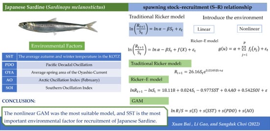
SST	The average autumn and winter temperature in the KOTZ
PDO	Pacific Decadal Oscillation
OYA	Average spring area of the Oyashio Current
AO	Arctic Oscillation Index (February)
SOI	Southern Oscillation Index
S-R	Spawning stock-recruitment

describes the abbreviations of fisheries and environmental data used in this study.

2.2. Model Building Process

In order to determine the optimal fitting model for S. melanostictus, the influence of environmental factors on S. melanostictus spawning stock recruitment was investigated. We constructed and compared different S-R models: the traditional Ricker model, the Ricker environment extension model (GLM method modeling), and the GAM model. The predictors of the recruitment models included stock biomass individually and the combination of stock biomass and marine environmental factors (SST, PDO, OYA, AO, and SOI). The best model was determined by comparing the explanatory and predictive power of the different structural candidate models (different numbers of environmental factors) against the traditional Ricker model. Through the analysis and comparison of different models, the model with the best fitting effect was selected to study recruitment. This study mainly used R (x64 version 4.1.1) and Origin for analysis.

In this study, a correlation test between environmental factors and recruitment was conducted using the Pearson correlation coefficient to screen the key environmental factors associated with recruitment. A Ricker type environmental extension model based on the traditional Ricker model was constructed using the glm() function and mgcv package. The variance inflation factor (VIF) was used to judge the collinearity numerically. Generally, a VIF <5 is considered to indicate no collinearity effect [37].

2.2.1. Ricker and Ricker-E Model

Both Beverton-Holt (B-H) [38] and Ricker [16] are models used to describe the S-R relationship [39,40]. However, the S-R relationship is not a simple density-dependent relationship, and researchers have gradually introduced environmental factors into the stock-recruitment model, to simultaneously consider the effects of density-dependent and environmental-dependent factors on the relationship of recruitment. The B-H and Ricker reproduction models were modified to explore the impact of the environment on the stock-recruitment relationship [41,42,43]. However, the latter is used more frequently, and Ricker is more appropriate for including environmental factors [44]; therefore, the Ricker model was chosen to describe the S-R relationship of S. melanostictus in this study.

$$R_{t+1}=\alpha S_t{e}^{-\beta S_t}\cdot e^{{\epsilon }_t\left(0,{\sigma }^2\right)}$$

(1)

where $R_{t+1}$ is the recruitment in the year $t+1$, $S_t$ is the spawning stock in year t, $\alpha$ and $\beta$ are parameters to be estimated, and $\epsilon$ is a normally distributed random error term, $\epsilon ~\mathrm{N}$ (0, ${\sigma }^2$).

Usually, Ricker allows the model to be estimated using linear regression, and Equation (2) was used to estimate the parameters for the regression analysis:

$$\ln \left(\frac{R_{t+1}}{S_t}\right)=ln \alpha -\beta S_t+{\epsilon }_t$$

(2)

The mechanism of S. melanostictus fluctuations is complex, and the density-constrained mechanism is not the direct cause affecting population fluctuations [45]. Sakuramoto et al. [24] suggested that the fundamental cause of S. melanostictus fluctuations in the Northwest Pacific Ocean is related to environmental conditions. Therefore, to explore the influence of environmental factors on S. melanostictus, we established an S-R model of environmental influence based on the Ricker model. The Ricker model equation incorporating environmental covariates is as follows:

$$\ln \left(\frac{R_{t+1}}{S_t}\right)=ln \alpha -\beta S_t+f\left(X\right)+{\epsilon }_t$$

(3)

The function $f\left(X\right)$ represents the effect of different marine environmental factors, $f\left(X\right)={\gamma }_1{X}_{t,1}+{\gamma }_2{X}_{t,2}+\cdots +{\gamma }_n{X}_{t,n}$, where $X_{t,1}$, $X_{t,2}$,$\dots ,$ $X_{t,n}$, represent environmental variables that may impact S-R during the year. Additionally, ${\gamma }_1$, ${\gamma }_2$, and $\dots {\gamma }_n$ denote the values of the corresponding environmental variable parameters.

2.2.2. GAM Model

The GAM is an extension of the GLM, which was used to study the environmental factors that affect the S-R of S. melanostictus. In general, GAM has more flexibility [46]. The GAM minimizes residuals (goodness of fit), while maximizing parsimony (lowest possible degrees of freedom) to detect nonlinear relationships between variables [47]. The expressions is as follows:

$$g\left(u\right)=\alpha +{\displaystyle \sum }_{j=1}^p{f}_{\dot{j}}\left(x_j\right)+{\epsilon }_t$$

(4)

where $g\left(u\right)$ is the desired response variable; (the Logarithm recruitment/spawning stock biomass in this study $\ln (\frac{R}{S})$, $f_j$ is each explanatory variable $x_j$ ($S_t,SST,PDO,OYA,AO,SOI$) of the smoothing function), and ${\epsilon }_t$ is a residual that follows a normal distribution. The effects of the spawning stock and environmental variables on recruitment were fitted using a cubic spline bs = “cr”, and an s (smoothing spline) was used as a smoother to estimate the S-R relationship.

2.3. Selection Criteria and Validation of Models

The Akaike information criterion (AIC) is essential in testing the significance of differences between models and is widely used to select optimal models [48]. Usually, the minimum value of the AIC represents a good fit for the model. The expressions is as follows:

$$AIC=2k-2\ln \left(L\right)$$

(5)

where k denotes the independent parameter format of the model and L denotes the great likelihood function of the model.

In this study, the AIC was the selection criterion for the best model. In the Ricker-E, the stepAIC () function of MASS was used to select the best model, considering various combinations of environmental factors. To improve the accuracy of the model, we used tenfold cross-validation. In the GAM, environmental factors were added to the model successively, until the AIC value was no longer decreased, and the optimal model was selected. Additionally, to ensure the accuracy of the selection results, the model was predicted for verification. Similarly, single and multivariate analyses were used separately in the GAM model building process. First, different numbers of environmental factors were added to the model successively, until the AIC value no longer decreased, and the optimal model was selected. Then, for the three S-R models with different structures, AIC was used as the judgment criterion to choose the optimal model. Lastly, we validated the model, to ensure the accuracy of the selection results.

3. Results

3.1. Screening of Environmental Factors

The results of the correlation analysis (Figure 2) showed that recruitment was significantly correlated with various environmental factors, except for SOI. At the same time, the effect of SST on recruitment showed a negative correlation (−0.714), even higher than the correlation coefficient between spawning stock and recruitment (0.629). On the other hand, the AO was positively correlated with recruitment, with a correlation coefficient of 0.438. In addition, the SOI had the smallest relationship with the recruitment, which was negative, with a correlation coefficient of −0.115. Therefore, SSB and environmental factors should be considered when investigating the S−R relationship in S. melanostictus [24]. The results also indicated that there may be interactions among the environmental factors (some environmental factors had large correlation coefficients with each other, such as AO and PDO, with a correlation coefficient of 0.779).

Figure 3 shows the overall decreasing trend in recruitment during the period of 1986−2013; after 2013, the recruitment increased under the general trend. However, the recruitment was on a downward trajectory, while the SST increased from 1986 to 1988. The SOI changed from a negative to a positive correlation from 1986 to 1988, and El Niño became La Niña during 2013−2018, with an overall fluctuating increase and a decrease in individual years.

3.2. Traditional Ricker Model

From 1984 to 2018, the Ricker curve of S. melanostictus showed the characteristics of the Ricker model dome (Figure 4). The S-R fit was satisfactory from 1992 to 2018, with observations distributed around the Ricker curve. However, before 1992, the fitted values had significant deviations, especially during the period from 1984 to 1991, in which the observed values were far from the Ricker curve, and the fit was poor. Therefore, we speculated that this might have been influenced by the marine environment. By fitting the traditional Ricker model, the AIC was 100.25, and the BIC was 104.91. The parameter estimation results showed that the α parameter was 26.16, and the β value was −0.0149. Therefore, the equation of the traditional Ricker model was as follows:

$$R_{t+1}=26.16S_t{\mathrm{e}}^{0.0149S_t+\epsilon }$$

(6)

3.3. Results of the Ricker Environment Extension Model

A stepwise regression analysis showed that the optimal Ricker-E model included three environmental variables (SST, AO, and SOI) that significantly affected the recruitment (p < 0.05) (

Table 2. Results of the best Ricker-E model with the addition of environmental factors in different numbers.

Formula	Variable	Estimate	Standard Error	t Value	Pr(>|t|)		VIF	AIC	BIC
ln(R/S) ~ S + SST		22.087	5.149	4.290	0.0002	***		90.00	96.20
	S	−0.024	0.004	−5.640	0.0000	***	1.51
	SST	−1.226	0.335	−3.660	0.0009	***	1.51
ln(R/S) ~ S + SST + AO	Intercept	17.293	5.645	3.060	0.0045	**		88.50	96.30
	S	−0.023	0.004	−5.600	0.0000	***	1.53
	SST	−0.918	0.366	−2.510	0.0176	*	1.93
	AO	0.283	0.157	1.800	0.0816	.	1.33
ln(R/S) ~ S + SST + AO + SOI	Intercept	18.118	5.287	3.430	0.0018	**		84.60	94.00
	S	−0.024	0.004	−6.206	0.0000	***	1.55
	SST	−0.977	0.343	−2.847	0.0079	**	1.94
	AO	0.400	0.155	2.575	0.0152	*	1.49
	SOI	0.542	0.231	2.346	0.0258	*	1.18

Note: Signif. codes: ‘***’ means p value ∈ [0, 0.001], ‘**’ means p value ∈ (0.001, 0.01], ‘*’ means p value ∈ (0.01, 0.05], ‘.’ means p value ∈ (0.05, 0.1], no cod means p value ∈ (0.1, 1).

). Moreover, the results of collinearity showed that the VIF was less than 5 during the modeling process, so there was no collinearity. The SST had the smallest p-value (0.0079) among the environmental variables, indicating that SST had the most significant influence on the dependent variable. The model fit AIC was 84.60. The expression of the Ricker-E model with the addition of environmental factors was as follows:

$$ln{R}_{t+1}-ln{S}_t=18.118+0.024S_t-0.977SST+0.4AO+0.542SOI+\epsilon$$

(7)

The points in Figure 5a are randomly distributed; therefore, there is no heteroskedasticity. The points in Figure 5b are distributed on the 45° diagonal, indicating that the sample approximately obeyed a normal distribution. Meanwhile, the points in Figure 5c are randomly distributed, and the maximum Cook distance in Figure 5d is approximately 0.3. We typically used 0.5 and 1 as the criteria for outliers [49]; therefore, there were no outliers.

We used tenfold cross-validation for model selection, using R-squared and RMSE as the judging criteria, and the results were the same as those of the models selected by stepwise regression. Table 2 shows the best Ricker-E models with the addition of different numbers of factors. A comparison of the best models in each group revealed that the model containing four factors had the largest R-squared (0.705) and the smallest RMSE (0.749) (

Table 3. Results of the tenfold cross-validation for the optimal Ricker-E model.

Nvmax	RMSE	Required	MAE	RMSESD	RsquaredSD	MAESD
1	0.931	0.686	0.747	0.334	0.338	0.277
2	0.789	0.610	0.653	0.365	0.323	0.292
3	0.935	0.653	0.781	0.299	0.282	0.264
4	0.749	0.705	0.617	0.264	0.297	0.235
5	0.806	0.641	0.668	0.331	0.295	0.286
6	0.820	0.656	0.687	0.299	0.285	0.263

Note: Nvmax represents the number of different factors added to the model.

). Furthermore, when five environmental factors were added, the RMSE and RMSESD became larger, and the Required became smaller. This indicated that the Ricker-E model with four factors (S, SST, AO, and SOI) was the optimal model.

3.4. Analysis Results of GAM

3.4.1. Single Factor Analysis of the GAM

Table 4. Results of the GAM single factor fit of S. melanostictus.

B.Smooth Terms	edf	Ref. df	F Value	p Value	GCV	Deviance Explained	Rsq.(adj)	AIC
s(S)	4.87	4.99	18.9	<2 × 10−16 ***	0.848	76.4%	0.724	94
s(SST)	5.98	6.67	6.32	<2 × 10−16 ***	1.484	61.7%	0.536	114
s(PDO)	1	1	11.16	<2 × 10−16 ***	2.094	25.20%	0.229	127
s(OYA)	5.95	6.62	2.16	<2 × 10−16 ***	2.487	35.8%	0.221	132
s(AO)	1	1	9.60	<2 × 10−16 ***	2.167	22.5%	0.202	128
s(SOI)	3.2	3.83	0.88	<2 × 10−16 ***	2.705	15.80%	0.070	136

Note: Signif. codes: ‘***’ means p value ∈ [0, 0.001].

shows that S had the largest explained deviation and Rsq.(adj), followed by SST with 76.40% and 61.70%, and 0.724 and 0.503, respectively. The results of the single factor analysis of the GAM showed that each environmental factor was statistically significant and had a significant effect (p < 0.05). In addition, the estimated degrees of freedom (edf) of PDO and AO were 1, indicating that PDO and AO had a linear relationship effect on ln(R/S) in the single factor model. Another factor, edf, was greater than 1, indicating nonlinear effects.

The trend in Figure 6a shows two peak values at 20 × 10² kt and 95 × 10² kt. Before 20 × 10² kt and between 48 × 10² kt and 95 × 10² kt, the ln(R/S) showed an increasing trend. Meanwhile, the periods of 20 × 10² kt–48 × 10² kt and 95 × 10² kt–130 × 10² kt showed a decreasing trend. Figure 6b shows that at 14.0 °C, the ln(R/S) was the highest, whereas, between 14 °C and 15 °C, the ln(R/S) rapidly decreased; between 15 °C and 16 °C SST, the ln(R/S) fluctuated after experiencing a reduction. Furthermore, the ln(R/S) decreased when temperatures surpassed 16 °C. Figure 6c,e show that the effects of PDO and AO on ln(R/S) exhibited an increasing linear trend; with an increase in the PDO and AO indices, while ln(R/S) also increased. Figure 6d shows the ln(R/S) fluctuating variation of OYA between 5 × 10⁴ km² and 15 × 10⁴ km². The OYA significantly increases in ln(R/S) after 15 × 10⁴ km² − 20 × 10⁴ km². Figure 6f shows a decreasing trend of ln(R/S) at the SOI of −0.6, with a change at −0.5. At less than −0.5, the ln(R/S) decreased with an increasing SOI; at an SOI greater than −0.5, there was a gradual positive correlation, with ln(R/S) increasing with SOI.

3.4.2. Multifactor Analysis

Table 5. Comparison of the best models with different numbers of factors in the GAM.

Model	Formula	edf	t Value	p	adjR2	Explained	AIC	BIC
GAM1	ln(R/S) ~ s(S)		32.2	***	0.72	76.40%	94.4	105.0
	s(S)	4.87		***
GAM2	ln(R/S) ~ s(S) + s(SST)		48.1	***	0.88	91.90%	70.6	91.8
	s(S)	4.91		***
	s(SST)	6.75		***
GAM3	ln(R/S) ~ s(S) + s(SST) + s(PDO)		50.9	***	0.89	93.40%	67.2	91.3
	s(S)	4.9		***
	s(SST)	6.72		***
	s(PDO)	1.83
GAM4	ln(R/S) ~ s(S) + s(SST) + s(PDO) + s(AO)		58.6	***	0.91	95.70%	57.9	86.7
	s(S)	4.83		***
	s(SST)	6.87		***
	s(PDO)	2.30		*
	s(AO)	2.49		.

Note: Signif. codes: ‘***’ means p value ∈ [0, 0.001], ‘**’ means p value ∈ (0.001, 0.01], ‘*’ means p value ∈ (0.01, 0.05], ‘.’ means p value ∈ (0.05, 0.1], no cod means p value ∈ (0.1, 1).

indicates that the best model for a single environmental factor was GAM2. Compared to GAM1, the AIC decreased from 94.4 to 70.6, while the R-sq. (adj) increased from 0.72 to 0.88, indicating a significantly improved fit with the addition of the environmental factor. After adding the remaining environmental factors to GAM2, the best model was GAM3, with a decrease in the AIC to 67.2 and an increase in R-sq. (adj). We found that, after adding four factors to GAM4 and then adding the environmental factors OYA and SOI, the AIC increased to 58.20 and 60.00, respectively. The R-sq. (adj) values did not increase significantly. Therefore, we determined that the model with the addition of four factors (GAM4) was the best. The GAM expression was as follows.

$$\ln (R/S)=s\left(S\right)+s\left(SST\right)+s\left(PDO\right)+s\left(AO\right).$$

(8)

Figure 7b indicates the highest values at 14.4 °C, corresponding to the highest ln(R/S). The ln(R/S) decreased significantly between 14.4 °C and 15 °C. It fluctuated between 15 °C and 16 °C, with two relatively small peaks at 15.3 °C and 15.9 °C. Figure 7c,d show that PDO and AO had opposite effects on ln(R/S). With a negative PDO index, ln(R/S) decreased, whereas, with a positive PDO index, ln(R/S) increases; AO was precisely the opposite of PDO. The visual analysis of Figure 7 revealed a possible interaction between the environmental factor SST and spawning (Figure 8a). Figure 8b shows a significant interaction between SST and spawning (p < 0.001), with either a too high or too low SST interacting with spawning, thus affecting the recruitment.

3.5. Fitting Verification of the Optimal Model

According to GAM single factor and multivariate analysis, GAM4 was the best model. A fitting test of the model was carried out to confirm the accuracy of the results. Figure 9 indicates the fit of the predicted values of the three models to the observed values, as well as the degree of fit of the three models to the recruitment varies. All three models were fitted well by the predictor variables after 1992. However, for the prediction of recruitment during 1984–1992, the fitted line of the traditional Ricker model (Figure 9a) was compared with the fitted line of the Ricker model, with the addition of environmental factors (Figure 9b). We found that the latter was less variable. As a result, the difference between the predicted and observed values was smaller, and the fitting effect was better. However, the fit of the GAM to recruitment (Figure 9c) showed a significantly better model fit with less variation than the previous two. This may be because environmental factors strongly influenced it before 1992, and the GAM had a better fit and better explained the effects of the environment on recruitment.

4. Discussion

4.1. S-R Model

The Ricker model is widely used to describe S-R relationships in stock assessment, but it is more inclined toward the influence of biological factors such as SSB on recruitment [50]. However, the influence of abiotic factors in the ecosystem, including the environment, food, and other factors on recruitment, cannot be ignored [51,52]. The GLM and GAM are widely used for studying environmental impacts on fisheries [53,54,55]. Langley et al. [56] developed a GLM to study changes in the recruitment of yellowfin tuna (Thunnus albacares) under changing marine environmental factors. In our study, a linear model (Ricker-E) and nonlinear model (GAM) were used to study the S-R relationship between the environment and S. melanostictus. The Ricker-E model fit better than the traditional Ricker model, which indicates that a model incorporating environmental variables better describes the S-R relationship [57]. The GAM had the smallest AIC (57.9), proving that the nonlinear model was better than the linear model. Deyle et al. [58] found that nonlinear (state-dependent) models produced better predictions than linear models, after studying environmental effects on sardine ichthyoplankton. Cardinale and Arrhenius [59] noted that the GAM was better than the Ricker-E model in describing the number of environmental strengths in the recruitment of cod. Megrey et al. [60] concluded that the GAM, a nonparametric approach, is better than parametric methods in predicting parameter estimates in recruitment intensity. Shih et al. [61] found that GAM could fit the data better than the linear model in their study of environmental effects on recruitment for North Pacific Albacore tuna (Thunnus alalunga). The fitting results (Figure 9) indicate that the nonlinear GAM had a smaller prediction error relative to the Ricker-E model and was the best model to describe the environment of the S-R relationship of S. melanostictus [62].

In addition, the interaction between environmental SST and S was determined through visualization of the optimal model (Figure 8). The highest value of SST in Figure 8 was approximately 14 °C. Therefore, SST was the main environmental factor influencing the S-R relationship in this study.

4.2. The Effect of the Environment on Recruitment

Small pelagic fish are susceptible to environmental changes, and warm and cold changes in seawater alter stratification, habitat, and biological rates, thereby affecting population changes in marine fish. Large-scale climate indices such as AO, PDO, and SOI have been widely demonstrated to affect population fluctuations of small pelagic fish, including sardines [34,63,64,65,66]. Yastu et al. [34] reported that a wide range of environmental indices, such as PDO and AO, may be helpful in understanding and predicting the effects of the environment on the productivity and recruitment of sardines.

4.2.1. Kuroshio Oyashio Regional

Jacobson and MacCall [67] showed that SST affects changes in the recruitment of Pacific sardines. As sardines spawn in winter or early spring near the Kuroshio in southern Japan, their juvenile and adult fish pass through the Kuroshio and Kuroshio extension, to feed in the Oyashio area [68,69]. Therefore, the SST in this study area is important for sardine recruitment. Takasuka [70] suggested that a cooler SST in winter spawning grounds improves the success rate of sardine recruitment. Water temperature and zooplankton abundance affect sardine survival during early growth stages (up to 1 year old) [71]. Typically, warm events are associated with low productivity, where the release of larval predators during warm periods outweighs the scarcity of food, thereby affecting the survival of eggs and larvae. Typically, the low productivity associated with warmth affects the survival rate of eggs and larvae [29,72]. Noto and Yasuda [73] indicated that winter–spring SST in the Kuroshio extension and its southern recirculation zone was positively correlated with the effect of natural mortality of S. melanostictus larvae from late stages to age 1. This study showed that SST was significantly correlated with S. melanostictus recruitment (p < 0.05), and that SST was the dominant environmental influence. Furthermore, the GAM results showed that ln(R/S) increased with increasing temperature and achieved a maximum of 14.4 °C. However, after a rapid decrease after reaching 14.4 °C, the rate of decline slowed down and fluctuated. We speculate that this elevated temperature may promote the growth of fish cells until a critical point is reached, but exceeding the critical point affects the metabolic rate of sardines, leading to a decrease in growth [74]. Takasuka et al. [21] stated that the optimal growth temperature for sardine larvae is 16.2 °C, while the maximum ln(R/S) achieved at 14.4 °C in this study may be the result of multifactorial climatic effects.

The dynamics of the OYA affect the migration and abundance of pelagic fish, through changes in primary productivity and mesopelagic biomass [75]. The results of the GAM single factor fit showed that the effect of the OYA on S. melanostictus recruitment was significant, with an explanation of variance of 35.8% (Table 4). This study found that the effect on recruitment was small and irregular when the OYA was small. However, with an area of 15 × 10⁴ km², recruitment tended to increase with increasing OYA (Figure 5d). The positive correlation between OYA and S. melanostictus recruitment at this point may be due to the low water temperature, low salinity, and rich nutrient characteristics of the Oyashio, which ensure sardine feeding.

4.2.2. Large-Scale Climatic Patterns

SST anomalies (cooling or warming) caused by alternating cold and warm PDO periods impact the temperature and location of fish spawning grounds. During positive PDO indices, cooler seas in the western North Pacific are favorable for sardine populations to flourish in Kuroshio systems [70]. Parrish [76] showed that the main positive PDO periods were associated with the accumulation of larger sardine biomass. However, the PDO was negative, and the SST gradually warmed, consistent with the rapid decline in sardine biomass [77]. Similarly, Figure 7c confirms this view. When the PDO index was at −1.5 to 0, the ln(R/S) showed a decreasing trend. In contrast, when the PDO index was positive, the ln(R/S) started to show an increasing trend. This indicates that the positive and negative PDO indices affected S. melanostictus population changes, with a positive direction favoring recruitment growth, and a negative direction inhibiting recruitment growth. Sardines are suited to living in cooler environments and grow more slowly in warmer environments [21]. During the negative PDO period, the population decline was due to low reproductive success, resulting in a total mortality exceeding recruitment. Pitcher and Hart [78] indicated that the highest correlation was between sardine recruitment during the spawning season and the PDO index, which may be related to the cumulative effect of the before-spawning environment on adult sardines. Interestingly, Sakuramoto [66] showed that the partial regression coefficients associated with PDO were not statistically significant in the S-R prediction model of S. melanostictus populations in the Pacific.

Table 2 shows that the AO was significantly correlated with the Ricker-E model fit (p < 0.015). In the GAM single factor fit, AO showed a positive linear correlation with ln(R/S) (Figure 6e). Meanwhile, the multifactor fit showed a nonlinear relationship and the opposite trend to the PDO variation. Positive PDO abnormalities imply low levels of recruitment, while negative abnormalities are associated with high levels. The AO tends to be in a positive phase when the stratospheric vortex is strong in winter [79]. A positive AO affects snow melting, resulting in a large runoff into the ocean and causing sea surface salinity, density, and temperature changes [80]. Negative AO affected recruitment by changing the food supply of sardines through cold air temperatures [81]. Many reports have shown that the AO affects different regional populations. Báez et al. [63] found that AO influenced the relative abundance of sardines in West Africa. Castro-Gutiérrez et al. [82] concluded that the extreme values (positive and negative) in the AO seemed to have a negative impact on the landings of European sardines in the same year.

Positive and negative changes in the SOI can lead to climate anomaly events, such as El Niño and La Niña, which manifest as large-scale persistent seawater anomalies. Large-scale ocean fluctuations such as ENSO events have been identified as possible causes of sardine population fluctuations in the Pacific Ocean [83,84]. The SOI had a significant effect on recruitment in the GAM single factor analysis (p < 0.05), but was not included in the final model in the multifactor analysis. The reason for this may be that its effect could not be highlighted under the combined influence of multiple factors or was replaced by other relevant strong environmental factors. There was an inflection point in the GAM single factor analysis when the SOI was positive or negative, where recruitment decreased and increased during El Niño, with the opposite trend during La Niña. El Niño events cause a weakening of cold currents and a decrease in upwelling, a decrease in the nutrient level of seawater, and an increase in the likelihood of extreme weather typhoons and storms. All of these factors have adverse effects on fish populations. Sogawa et al. [85] reported that the bottom-up effects of Kuroshio and Kuroshio extension areas supported the high productivity of sardines. The decrease in sea surface winter temperature caused by La Niña provides a suitable living environment for sardines. Consequently, there is an increase in recruitment. However, successive La Niña events caused sea surface temperatures to continue to decrease, at which point the temperature was no longer suitable for sardine survival and growth. In contrast with our conclusion, Deyle et al. [58] identified the SOI as one of the three variables least important for sardine dynamics, with a strong negative impact on prediction.

The influence of the marine environment on the population dynamics of S. melanostictus is complex. Uncertainties in fishery stock assessment and management cannot be ignored [86]. Sun et al. [87] developed harvest control rules based on management objectives, to control the impact of uncertainty. Environmentally induced changes in recruitment are one source of uncertainty in fishery stock assessment and management. Therefore, it is necessary to incorporate uncertain factors such as the environment into the evaluation management framework [88,89]. Tanaka et al. [90] used a bioclimate envelope model to confirm that climate change drove changes in habitat suitability, which favored increased recruitment of lobsters. This suggests that incorporating environmental variables into stock assessments and fisheries management can provide a more accurate picture of stock status. Siple et al. [91] also demonstrated that the inclusion of uncertainties, such as the environment in the management framework for assessing pelagic fish, can improve the accuracy of assessments. We can then include other issues that may create uncertainty in the fishery (species distribution, predator models, etc.) into the integrated management target system. There may be a delay in the current year’s environmental influences on recruitment, especially with regard to the large-scale climate. In this study, we did not consider lags in environmental impacts. Therefore, we will consider the delay of environmental factors in future studies, to ensure that more accurate prediction models are developed to explore the environmental effects on the S-R relationship of S. melanostictus.

5. Conclusions

This paper used estimates of stock/recruitment density for S. melanostictus, as well as matching environmental data collected from 1980 to 2018. We fitted the Ricker-E, GAM, and traditional Ricker models to fit models to these data. The results showed that the nonlinear GAM was the most suitable model to describe changes in the recruitment of S. melanostictus under environmental influences. SST, PDO, and AO are environmental factors that influence the level of recruitment. Among them, SST is the most important environmental factor, with a negative impact on the level of recruitment. This has important implications for studying the recruitment changes of S. melanostictus under the influence of the marine environment.

References

- Brander, K. Impacts of climate change on fisheries. J. Mar. Syst. 2010, 79, 389–402. [Google Scholar] [CrossRef]
- Alheit, J. Consequences of regime shifts for marine food webs. Int. J. Earth Sci. 2009, 98, 261–268. [Google Scholar] [CrossRef]
- Kawasaki, T. Recovery and collapse of the Far Eastern sardine. Fish. Oceanogr. 1993, 2, 244–253. [Google Scholar] [CrossRef]
- Alheit, J.; Pohlmann, T.; Casini, M.; Greve, W.; Hinrichs, R.; Mathis, M.; O’Driscoll, K.; Vorberg, R.; Wagner, C. Climate variability drives anchovies and sardines into the North and Baltic Seas. Prog. Oceanogr. 2012, 96, 128–139. [Google Scholar] [CrossRef]
- Barange, M.; Bernal, M.; Cercole, M.C.; Cubillos, L.A.; Daskalov, G.M.; Cunningham, C.L.; de Oliveira, J.A.; Dickey-Collas, M.; Gaughan, D.J.; Hill, K. Current trends in the assessment and management of stocks. In Climate Change and Small Pelagic Fish; Cambridge University Press: Cambridge, UK, 2009; pp. 191–255. [Google Scholar] [CrossRef]
- Allain, G.; Petitgas, P.; Lazure, P. The influence of mesoscale ocean processes on anchovy (Engraulis encrasicolus) recruitment in the Bay of Biscay estimated with a three-dimensional hydrodynamic mode. Fish. Oceanogr. 2001, 10, 151–163. [Google Scholar] [CrossRef]
- Zhao, X.; Hamre, J.; Li, F.; Jin, X.; Tang, Q. Recruitment, sustainable yield and possible ecological consequences of the sharp decline of the anchovy (Engraulis japonicus) stock in the Yellow Sea in the 1990s. Fish. Oceanogr. 2003, 12, 495–501. [Google Scholar] [CrossRef]
- Takasuka, A.; Oozeki, Y.; Kimura, R.; Kubota, H.; Aoki, I. Growth-selective predation hypothesis revisited for larval anchovy in offshore waters: Cannibalism by juveniles versus predation by skipjack tunas. Mar. Ecol. Prog. Ser. 2004, 278, 297–302. [Google Scholar] [CrossRef] [Green Version]
- Checkley, D.M., Jr.; Bakun, A.; Barange, M.A.; Castro, L.R.; Fréon, P.; Guevara-Carrasco, R.; Herrick, S.F., Jr.; MacCall, A.D.; Ommer, R.; Oozeki, Y. Climate Change and Small Pelagic Fish. Cambridge University Press: Cambridge, UK, 2009; pp. 999–1000. [Google Scholar] [CrossRef]
- Funamoto, T.; Aoki, I. Reproductive ecology of Japanese anchovy off the Pacific coast of eastern Honshu, Japan. J. Fish Biol. 2002, 60, 154–169. [Google Scholar] [CrossRef]
- Silva, A. Morphometric variation among sardine (Sardina pilchardus) populations from the northeastern Atlantic and the western Mediterranean. ICES J. Mar. Sci. 2003, 60, 1352–1360. [Google Scholar] [CrossRef]
- Ganias, K.; Somarakis, S.; Machias, A.; Theodorou, A. Evaluation of spawning frequency in a Mediterranean sardine population (Sardina pilchardus sardina). Mar. Biol. 2003, 142, 1169–1179. [Google Scholar] [CrossRef]
- Miranda, A.; Cal, R.M.; Iglesias, J. Effect of temperature on the development of eggs and larvae of sardine Sardina pilchardus Walbaum in captivity. J. Exp. Mar. Biol. Ecol. 1990, 140, 69–77. [Google Scholar] [CrossRef]
- Santos, M.B.; González-Quirós, R.; Riveiro, I.; Cabanas, J.M.; Porteiro, C.; Pierce, G.J. Cycles, trends, and residual variation in the Iberian sardine (Sardina pilchardus) recruitment series and their relationship with the environment. ICES J. Mar. Sci. 2012, 69, 739–750. [Google Scholar] [CrossRef] [Green Version]
- Morimoto, H. Age and growth of Japanese sardine Sardinops melanostictus in Tosa Bay, southwestern Japan during a period of declining stock size. Fish. Sci. 2003, 69, 745–754. [Google Scholar] [CrossRef] [Green Version]
- Ricker, W.E. Computation and interpretation of biological statistics of fish populations. Bull. Fish. Res. Board Can. 1975, 191, 1–382. [Google Scholar] [CrossRef]
- Lee, H.-H.; Maunder, M.N.; Piner, K.R.; Methot, R.D. Can steepness of the stock-recruitment relationship be estimated in fishery stock assessment models? Fish. Res. 2012, 125, 254–261. [Google Scholar] [CrossRef]
- Nishikawa, H. Relationship between recruitment of Japanese sardine (Sardinops melanostictus) and environment of larval habitat in the low-stock period (1995–2010). Fish. Oceanogr. 2019, 28, 131–142. [Google Scholar] [CrossRef] [Green Version]
- Wada, T.; Jacobson, L.D. Regimes and stock-recruitment relationships in Japanese sardine (Sardinops melanostictus), 1951–1995. Can. J. Fish. Aquat. Sci. 1998, 55, 2455–2463. [Google Scholar] [CrossRef]
- Ganias, K. Linking sardine spawning dynamics to environmental variability. Estuar. Coast. Shelf Sci. 2009, 84, 402–408. [Google Scholar] [CrossRef]
- Takasuka, A.; Oozeki, Y.; Aoki, I. Optimal growth temperature hypothesis: Why do anchovy flourish and sardine collapse or vice versa under the same ocean regime? Can. J. Fish. Aquat. Sci. 2007, 64, 768–776. [Google Scholar] [CrossRef]
- Grip, K.; Blomqvist, S. Marine nature conservation and conflicts with fisheries. Ambio 2020, 49, 1328–1340. [Google Scholar] [CrossRef] [PubMed] [Green Version]
- Salinger, M. A brief introduction to the issue of climate and marine fisheries. Clim. Chang. 2013, 119, 23–35. [Google Scholar] [CrossRef]
- Sakuramoto, K.; Shimoyama, S.; Suzuki, N. Relationships between environmental conditions and fluctuations in the recruitment of Japanese sardine, Sardinops melanostictus, in the northwestern Pacific. Bull. Jpn. Soc. Fish. Oceanogr. 2010, 74, 88–97. [Google Scholar]
- McClatchie, S.; Goericke, R.; Auad, G.; Hill, K. Re-assessment of the stock-recruit and temperature-recruit relationships for Pacific sardine (Sardinops sagax). Can. J. Fish. Aquat. Sci. 2010, 67, 1782–1790. [Google Scholar] [CrossRef]
- Lindegren, M.; Checkley, D.M., Jr. Temperature dependence of Pacific sardine (Sardinops sagax) recruitment in the California Current Ecosystem revisited and revised. Can. J. Fish. Aquat. Sci. 2013, 70, 245–252. [Google Scholar] [CrossRef] [Green Version]
- Daskalov, G.; Boyer, D.; Roux, J. Relating sardine Sardinops sagax abundance to environmental indices in northern Benguela. Prog. Oceanogr. 2003, 59, 257–274. [Google Scholar] [CrossRef]
- Nishikawa, H.; Yasuda, I. Japanese sardine (Sardinops melanostictus) mortality in relation to the winter mixed layer depth in the Kuroshio Extension region. Fish. Oceanogr. 2008, 17, 411–420. [Google Scholar] [CrossRef]
- Nishikawa, H.; Yasuda, I.; Itoh, S. Impact of winter-to-spring environmental variability along the Kuroshio jet on the recruitment of Japanese sardine (Sardinops melanostictus). Fish. Oceanogr. 2011, 20, 570–582. [Google Scholar] [CrossRef]
- Nakayama, S.I.; Takasuka, A.; Ichinokawa, M.; Okamura, H. Climate change and interspecific interactions drive species alternations between anchovy and sardine in the western North Pacific: Detection of causality by convergent cross mapping. Fish. Oceanogr. 2018, 27, 312–322. [Google Scholar] [CrossRef]
- Asia-Pacific Data-Research Center of the IPRC. Available online: http://apdrc.soest.hawaii.edu/ (accessed on 12 January 2022).
- Japan Meteorological Agency. Available online: https://www.data.jma.go.jp/gmd/kaiyou/data/shindan/b_2/oyashio_exp/oyashio_exp.html (accessed on 25 October 2021).
- NOAA National Centers for Environmental Information. Available online: https://www.ncdc.noaa.gov (accessed on 25 October 2021).
- Yatsu, A.; Watanabe, T.; Ishida, M.; Sugisaki, H.; Jacobson, L.D. Environmental effects on recruitment and productivity of Japanese sardine Sardinops melanostictus and chub mackerel Scomber japonicus with recommendations for management. Fish. Oceanogr. 2005, 14, 263–278. [Google Scholar] [CrossRef]
- Brander, K.; Mohn, R. Effect of the North Atlantic Oscillation on recruitment of Atlantic cod (Gadus morhua). Can. J. Fish. Aquat. Sci. 2004, 61, 1558–1564. [Google Scholar] [CrossRef]
- Watanabe, Y.; Zenitani, H.; Kimura, R. Population decline off the Japanese sardine Sardinops melanostictus owing to recruitment failures. Can. J. Fish. Aquat. Sci. 1995, 52, 1609–1616. [Google Scholar] [CrossRef]
- Cornic, M.; Rooker, J.R. Influence of oceanographic conditions on the distribution and abundance of blackfin tuna (Thunnus atlanticus) larvae in the Gulf of Mexico. Fish. Res. 2018, 201, 1–10. [Google Scholar] [CrossRef]
- Hilborn, R.; Walters, C.J. Quantitative Fisheries Stock Assessment: Choice, Dynamics and Uncertainty; Springer: New York, NY, USA, 1992; Volume 2, pp. 177–178. [Google Scholar]
- Ricker, W.E. Stock and recruitment. J. Fish. Res. Board Can. 1954, 11, 559–623. [Google Scholar] [CrossRef]
- Beverton, R.J.; Holt, S.J. On the dynamics of exploited fish populations. Rev. Fish Biol. Fish. 1994, 4, 259–260. [Google Scholar] [CrossRef]
- Schweight, J.F.; Noakes, D.J. Forecasting pacific herring (Cuplea arengus pallasi) recruitment from spawner abundance and environmental information. In Proceedings of the International Herring Symposium, Anchorage, AK, USA, 23–25 October 1990; pp. 373–387. [Google Scholar]
- Williams, E.H.; Quinn, T.J., II. Pacific herring, Clupea pallasi, recruitment in the Bering Sea and north-east Pacific Ocean, II: Relationships to environmental variables and implications for forecasting. Fish. Oceanogr. 2000, 9, 300–315. [Google Scholar] [CrossRef]
- Solow, A.R. Fisheries recruitment and the North Atlantic oscillation. Fish. Res. 2002, 54, 295–297. [Google Scholar] [CrossRef]
- Arregui, I.; Arrizabalaga, H.; Kirby, D.S.; Martín-González, J.M. Stock-environment-recruitment models for North Atlantic albacore (Thunnus alalunga). Fish. Oceanogr. 2006, 15, 402–412. [Google Scholar] [CrossRef]
- Sakuramoto, K. Does the Ricker or Beverton and Holt type of stock-recruitment relationship truly exist? Fish. Sci. 2005, 71, 577–592. [Google Scholar] [CrossRef]
- Beck, N.; Jackman, S. Beyond linearity by default: Generalized additive models. Am. J. Political Sci. 1998, 42, 596–627. [Google Scholar] [CrossRef]
- Coupé, C. Modeling linguistic variables with regression models: Addressing non-Gaussian distributions, non-independent observations, and non-linear predictors with random effects and generalized additive models for location, scale, and shape. Front. Psychol. 2018, 9, 513. [Google Scholar] [CrossRef] [Green Version]
- Akaike, H. A new look at the statistical model identification. IEEE Trans. Autom. Control. 1974, 19, 716–723. [Google Scholar] [CrossRef]
- Pinho, L.G.B.; Nobre, J.S.; Singer, J.M. Cook’s distance for generalized linear mixed models. Comput. Stat. Data Anal. 2015, 82, 126–136. [Google Scholar] [CrossRef]
- Fogarty, M.J. Recruitment in randomly varying environments. ICES J. Mar. Sci. 1993, 50, 247–260. [Google Scholar] [CrossRef]
- Shimoyama, S.; Sakuramoto, K.; Suzuki, N. Proposal for stock-recruitment relationship for Japanese sardine Sardinops melanostictus in North-western Pacific. Fish. Sci. 2007, 73, 1035–1041. [Google Scholar] [CrossRef]
- Myers, R.A. Stock and recruitment: Generalizations about maximum reproductive rate, density dependence, and variability using meta-analytic approaches. ICES J. Mar. Sci. 2001, 58, 937–951. [Google Scholar] [CrossRef] [Green Version]
- Yamada, H.; Takagi, N.; Nishimura, D. Recruitment abundance index of Pacific bluefin tuna using fisheries data on juveniles. Fish. Sci. 2006, 72, 333–341. [Google Scholar] [CrossRef]
- Solanki, H.; Bhatpuria, D.; Chauhan, P. Applications of generalized additive model (GAM) to satellite-derived variables and fishery data for prediction of fishery resources distributions in the Arabian Sea. Geocarto Int. 2017, 32, 30–43. [Google Scholar] [CrossRef]
- Sparholt, H. Causal correlation between recruitment and spawning stock size of central Baltic cod? ICES J. Mar. Sci. 1996, 53, 771–779. [Google Scholar] [CrossRef] [Green Version]
- Langley, A.; Briand, K.; Kirby, D.S.; Murtugudde, R. Influence of oceanographic variability on recruitment of yellowfin tuna (Thunnus albacares) in the western and central Pacific Ocean. Can. J. Fish. Aquat. Sci. 2009, 66, 1462–1477. [Google Scholar] [CrossRef]
- Chen, D.; Irvine, J. A semiparametric model to examine stock recruitment relationships incorporating environmental data. Can. J. Fish. Aquat. Sci. 2001, 58, 1178–1186. [Google Scholar] [CrossRef]
- Deyle, E.R.; Fogarty, M.; Hsieh, C.-H.; Kaufman, L.; MacCall, A.D.; Munch, S.B.; Perretti, C.T.; Ye, H.; Sugihara, G. Predicting climate effects on Pacific sardine. Proc. Natl. Acad. Sci. USA 2013, 110, 6430–6435. [Google Scholar] [CrossRef] [PubMed] [Green Version]
- Cardinale, M.; Arrhenius, F. The influence of stock structure and environmental conditions on the recruitment process of Baltic cod estimated using a generalized additive model. Can. J. Fish. Aquat. Sci. 2000, 57, 2402–2409. [Google Scholar] [CrossRef]
- Megrey, B.A.; Lee, Y.-W.; Macklin, S.A. Comparative analysis of statistical tools to identify recruitment-environment relationships and forecast recruitment strength. ICES J. Mar. Sci. 2005, 62, 1256–1269. [Google Scholar] [CrossRef]
- Shih, C.-L.; Chen, Y.-H.; Chien-Chung, H. Modeling the effect of environmental factors on the ricker stock-recruitment relationship for North Pacific albacore using generalized additive models. TAO Terr. Atmos. Ocean. Sci. 2014, 25, 581. [Google Scholar] [CrossRef] [Green Version]
- Murase, H.; Nagashima, H.; Yonezaki, S.; Matsukura, R.; Kitakado, T. Application of a generalized additive model (GAM) to reveal relationships between environmental factors and distributions of pelagic fish and krill: A case study in Sendai Bay, Japan. ICES J. Mar. Sci. 2009, 66, 1417–1424. [Google Scholar] [CrossRef] [Green Version]
- Báez, J.; Santamaría, M.; García, A.; González, J.; Hernández, E.; Ferri-Yáñez, F. Influence of the arctic oscillations on the sardine off Northwest Africa during the period 1976–1996. Vie Et Milieu. 2019, 69, 71–77. [Google Scholar]
- Zwolinski, J.P.; Demer, D.A. Environmental and parental control of Pacific sardine (Sardinops sagax) recruitment. ICES J. Mar. Sci. 2014, 71, 2198–2207. [Google Scholar] [CrossRef] [Green Version]
- Chavez, F.P.; Ryan, J.; Lluch-Cota, S.E.; Ñiquen, C.M. From anchovies to sardines and back: Multidecadal change in the Pacific Ocean. Science 2003, 299, 217–221. [Google Scholar] [CrossRef] [Green Version]
- Sakuramoto, K. A recruitment forecasting model for the Pacific stock of the Japanese sardine (Sardinops melanostictus) that does not assume density-dependent effects. Agri. Sci. 2013, 4, 1–8. [Google Scholar] [CrossRef]
- Jacobson, L.D.; MacCall, A.D. Erratum: Stock-recruitment models for Pacific sardine (Sardinops sagax). Can. J. Fish. Aquat. Sci. 1995, 52, 2062. [Google Scholar] [CrossRef]
- Yasuda, I.; Sugisaki, H.; Watanabe, Y.; MINOBE, S.S.; Oozeki, Y. Interdecadal variations in Japanese sardine and ocean/climate. Fish. Oceanogr. 1999, 8, 18–24. [Google Scholar] [CrossRef]
- Okunishi, T.; Ito, S.-i.; Hashioka, T.; Sakamoto, T.T.; Yoshie, N.; Sumata, H.; Yara, Y.; Okada, N.; Yamanaka, Y. Impacts of climate change on growth, migration and recruitment success of Japanese sardine (Sardinops melanostictus) in the western North Pacific. Clim. Chang. 2012, 115, 485–503. [Google Scholar] [CrossRef]
- Takasuka, A. Biological mechanisms underlying climate impacts on population dynamics of small pelagic fish. In Fish Population Dynamics, Monitoring and Management; Springer Nature: Tokyo, Japan, 2018; pp. 19–50. [Google Scholar] [CrossRef]
- Sunami, Y. Modeling of the variability in stock abundance of Japanese sardine from a viewpoint of its food density. J. Shimonoseki Univ. Fish. 1993, 41, 1–8. [Google Scholar]
- Bakun, A.; Broad, K. Environmental ‘loopholes’ and fish population dynamics: Comparative pattern recognition with focus on El Niño effects in the Pacific. Fish. Oceanogr. 2003, 12, 458–473. [Google Scholar] [CrossRef]
- Noto, M.; Yasuda, I. Population decline of the Japanese sardine, Sardinops melanostictus, in relation to sea surface temperature in the Kuroshio Extension. Can. J. Fish. Aquat. Sci. 1999, 56, 973–983. [Google Scholar] [CrossRef]
- Brett, J. Environmental factors and growth. In Fish Physiology: Bioenergetics and Growth; Academic Press: Cambridge, MA, USA, 1979; Volume 8, pp. 599–677. [Google Scholar] [CrossRef]
- Sakurai, Y. An overview of the Oyashio ecosystem. Deep Sea Res. Part II Top. Stud. Oceanogr. 2007, 54, 2526–2542. [Google Scholar] [CrossRef] [Green Version]
- Parrish, R.H. A Monterey sardine story. JB Phillips Hist. Fish. Rep. 2000, 1, 2–4. [Google Scholar]
- Hill, K.T.; Lo, N.C.; Macewicz, B.J.; Crone, P.R.; Felix-Uraga, R. Assessment of the Pacific Sardine Resource in 2009 for US Management in 2010: Executive Summary. 2009. Available online: https://repository.library.noaa.gov/view/noaa/3920 (accessed on 9 June 2022).
- Pitcher, T.; Hart, P. Fisheries Ecology; Croom Helm: London, UK, 1982. [Google Scholar]
- Douville, H. Stratospheric polar vortex influence on Northern Hemisphere winter climate variability. Geophys. Res. Lett. 2009, 36. [Google Scholar] [CrossRef] [Green Version]
- Báez, J.C.; Gimeno, L.; Gómez-Gesteira, M.; Ferri-Yáñez, F.; Real, R. Combined effects of the North Atlantic Oscillation and the Arctic Oscillation on sea surface temperature in the Alborán Sea. PLoS ONE 2013, 8, e62201. [Google Scholar] [CrossRef] [Green Version]
- Ohshimo, S.; Tanaka, H.; Hiyama, Y. Long-term stock assessment and growth changes of the Japanese sardine (Sardinops melanostictus) in the Sea of Japan and East China Sea from 1953 to 2006. Fish. Oceanogr. 2009, 18, 346–358. [Google Scholar] [CrossRef]
- Castro-Gutiérrez, J.; Cabrera-Castro, R.; Czerwinski, I.A.; Báez, J.C. Effect of climatic oscillations on small pelagic fisheries and its economic profit in the Gulf of Cadiz. Int. J. Biometeorol. 2022, 66, 613–626. [Google Scholar] [CrossRef] [PubMed]
- Cisneros-Mata, M.; Montemayor-López, G.; Nevárez-Martínez, M. Modeling deterministic effects of age-structure, density-dependence, environmental forcing and fishing on the population dynamics of Sardinops sagax caerulens in the Gulf of California. Calif. Coop. Ocean. Fish. Investig. Rep. 1996, 37, 201–208. [Google Scholar]
- Lluch-Belda, D.; Magallón, F.J.; Schwartzlose, R.A. Large fluctuations in the sardine fishery in the Gulf of California: Possible causes. CalCOFI Rep. 1986, 27, 136–140. [Google Scholar]
- Sogawa, S.; Hidaka, K.; Kamimura, Y.; Takahashi, M.; Saito, H.; Okazaki, Y.; Shimizu, Y.; Setou, T. Environmental characteristics of spawning and nursery grounds of Japanese sardine and mackerels in the Kuroshio and Kuroshio Extension area. Fish. Oceanogr. 2019, 28, 454–467. [Google Scholar] [CrossRef]
- Patterson, K.; Cook, R.; Darby, C.; Gavaris, S.; Kell, L.; Lewy, P.; Mesnil, B.; Punt, A.; Restrepo, V.; Skagen, D.W. Estimating uncertainty in fish stock assessment and forecasting. Fish Fish. 2001, 2, 125–157. [Google Scholar] [CrossRef]
- Sun, M.; Li, Y.; Ren, Y.; Chen, Y. Rebuilding depleted fisheries towards BMSY under uncertainty: Harvest control rules outperform combined management measures. ICES J. Mar. Sci. 2021, 78, 2218–2232. [Google Scholar] [CrossRef]
- Cao, J.; Chen, Y.; Richards, R.A. Improving assessment of Pandalus stocks using a seasonal, size-structured assessment model with environmental variables. Part I: Model description and application. Can. J. Fish. Aquat. Sci. 2017, 74, 349–362. [Google Scholar] [CrossRef]
- Cao, J.; Chen, Y.; Richards, R.A. Improving assessment of Pandalus stocks using a seasonal, size-structured assessment model with environmental variables. Part II: Model evaluation and simulation. Can. J. Fish. Aquat. Sci. 2017, 74, 363–376. [Google Scholar] [CrossRef] [Green Version]
- Tanaka, K.R.; Cao, J.; Shank, B.V.; Truesdell, S.B.; Mazur, M.D.; Xu, L.; Chen, Y. A model-based approach to incorporate environmental variability into assessment of a commercial fishery: A case study with the American lobster fishery in the Gulf of Maine and Georges Bank. ICES J. Mar. Sci. 2019, 76, 884–896. [Google Scholar] [CrossRef]
- Siple, M.C.; Koehn, L.E.; Johnson, K.F.; Punt, A.E.; Canales, T.M.; Carpi, P.; de Moor, C.L.; De Oliveira, J.A.; Gao, J.; Jacobsen, N.S. Considerations for management strategy evaluation for small pelagic fishes. Fish Fish. 2021, 22, 1167–1186. [Google Scholar] [CrossRef]