
Modeling Environmental Impacts of Intensive Shrimp Aquaculture: A Three-Dimensional Hydrodynamic Ecosystem Approach

1
Institute of Industrial Science, The University of Tokyo, 5-1-5 Kashiwanoha, Chiba 277-8574, Japan
2
Department of Systems Innovation, Graduate School of Engineering, The University of Tokyo, 5-1-5 Kashiwanoha, Chiba 277-8574, Japan
*
Author to whom correspondence should be addressed.
Fishes 2024, 9(4), 126; https://doi.org/10.3390/fishes9040126
Submission received: 29 February 2024
/
Revised: 28 March 2024
/
Accepted: 29 March 2024
/
Published: 31 March 2024
(This article belongs to the Section Fishery Economics, Policy, and Management)
Abstract
:Already a multibillion-dollar global industry, shrimp aquaculture, is growing all the time. The intensive method, which is the most common method in shrimp aquaculture, remains commercially challenged due to the expenditures associated with environmental pollution abatement. Although the comprehensive understanding of this intricate aquaculture environment has been advanced using mathematical modeling, recent attempts to improve the model’s structure have not yielded enough results. This work upgraded the previous method to a three-dimensional hydrodynamic ecosystem model with the effects of shrimps being replaced by approximation equations for the environmental assessment of a shrimp aquaculture pond in Kyushu District, Japan. Our approach was successful, as demonstrated by the high consistency of the simulation results when compared to observation data and the previous results. Additionally, we first revealed the impacts of stratification and confirmed the notable daily variation in the water quality. Our case study offers significant practical information on the characteristics of intensive shrimp aquaculture, implications for long-term sustainable operations, and future research priorities on local-scale ecosystem modeling.
Key Contribution: The development of a three-dimensional model in our case study reveals the effects of stratification and enables the optimization of paddle wheel aerator placement and quantity in wastewater treatment ponds, ultimately leading to more efficient energy consumption.
1. Introduction
Shrimp aquaculture is currently a multimillion-dollar worldwide industry that is expanding continuously. The financial prospect of shrimp aquaculture, which has already reached US $ 19.4 billion in 2017 between Europe and Asia, is drawing public attention thanks to a National Geographic documentary [1] that clearly illustrates the wide area of this industry in Indonesia. Similarly, the Mekong, Red River, Pearl River, and Yellow River Deltas have been reported to have 2659, 299, 1050, and 863 km2 of shrimp aquaculture, respectively [2]. Among these areas, penaeid shrimp, particularly Pacific white shrimp, are the most commonly farmed, and their production has propelled global shrimp production to a record high of 9.4 million tons in 2022 (FishStatJ; https://www.fao.org/fishery/en/topic/166235?lang=en (accessed on 31 January 2024)). More importantly, the growing demand in the global market continues to fuel the development of the shrimp business and aquaculture.
The penaeid shrimp aquaculture, based on major economic and technological differences, can be divided into extensive (relatively low levels of farming density), semi-intensive (intermediate levels of farming density), and intensive farming (relatively high levels of farming density) [3]. Extensive farming systems rely on traditional methods with minimal modifications, operating at low densities and inputs. They contribute negligibly to ecosystem nutrient and organic matter loads, primarily utilizing natural pond productivity supplemented occasionally with fertilizers. In contrast, intensive farming involves higher densities and inputs, including pelletized feed and chemicals/drugs, leading to increased nutrient and organic matter loads in the ecosystem [4]. The overloading has been linked to recorded cases of anoxic sediments and virus-related disease [4,5,6]. Solutions have been employed thus far, including paddle-wheel aerators for oxygen supply, regular water quality monitoring, and manual cleaning of anoxic sediments. However, these pollution abatement costs still challenge the commercial viability of intensive shrimp aquaculture [3].
To overcome the environmental problem, an advanced understanding of ecology, biology, and the environment is required [7,8,9]. This knowledge exploration involves synthesizing empirical data, assessing hypotheses, and understanding system dynamics, for which mathematical modeling is powerful [10,11]. When Burford et al. [12], for example, combined process measurements and bioindicators with data on water quality, they found that the ecological effects of changes in water quality parameters were oversimplified and recommended using phytoplankton responses and zooplankton communities for a more thorough assessment. Burford and Lorenzen [13] continued to develop a mathematical model to study nitrogen cycles, which included shrimp excretion, wasted feed decomposition, phytoplankton uptake, sedimentation, and remineralization. They concluded that sediment acted as a net sink of nitrogen across the whole production cycle. These ecosystem components were further calculated following water flow in a one-dimensional hydrodynamic-ecosystem coupled model by Kitazawa et al. [14]. Based on the nitrogen cycle and time-series nutrient results, it was reasonably explained that there was an approximately 100-fold increase in phytoplankton production in the shrimp aquaculture pond. Such a one-dimensional model also cannot be used to consider a management strategy of habitat for shrimps using equipment such as circulators and aerators, which create a three-dimensional environmental structure in a shrimp aquaculture pond [15,16].
Unfortunately, the overall knowledge has not significantly advanced since then, despite increased efforts to refine the model’s structure. Studies conducted after 2010, to the best of our knowledge, have focused more on the circulation of nutrients as a measure of water quality. Using the STELLA software Research version 8, Kittiwanich et al. [17] assessed the impact of nitrogen intake from feed on the nutrient dynamics of a well-aerated, enclosed shrimp pond in Thailand. Similar initiatives have been undertaken in Brazil [18] and Iran [19]. These calculations relied mostly on differential equations to describe the major nitrogen components, as with contemporary in-house models [20,21,22]. Perhaps as a result of their efforts, the growth modeling of shrimp has been substantially developed in the meantime to further assess the shrimp’s impacts on nutrient intake [23,24,25]. However, both fields—direct assessment (water quality) and indirect evaluation (shrimp growth)—are adopting artificial intelligence-related technologies, including the Bayesian hierarchical approach [26], the deep learning-based approach [27], and artificial neural network modeling [28]. Despite that, little research has been done to improve the spatial dimension of ecosystem modeling at the pond scale.
The present work aimed to clarify how the application of a three-dimensional hydrodynamic ecosystem model might enhance the previous calculation of the intensive aquaculture pond of penaeid shrimp [14]. The target penaeid shrimp is Penaeus japonicus, and the aquaculture pond was situated in the Kyushu district, Japan. Nevertheless, in the current three-dimensional hydrodynamic ecosystem model, the effects of shrimps were replaced by approximation differential equations. The numerical reproduction of the flow pattern at the surface, four water quality parameters, and the benthic sludge accumulation were all examined using the previous monitoring data. The advantages and disadvantages have been evaluated in contrast with the previous results. Based on the discussion, long-term sustainable operations and future research objectives have been suggested.
2. Materials and Methods
The previous one-dimensional model has been upgraded to a three-dimensional hydrodynamic ecosystem model, currently named the MEC (Marine Environmental Committee) Ocean model. This model has already incorporated hydrodynamic and lower trophic ecosystem components. Meanwhile, the previous shrimp growth sub-models have been replaced by approximation equations with evidenced-based parameter values. Finally, the model has been applied to the identical study case with a prolonged calculation period.
2.1. Three-Dimensional Hydrodynamic Ecosystem Model
The time variations in the vertical profiles of water temperature, salinity, density, and horizontal current velocity constitute the foundation of the hydrodynamic sub-model. These equations include the momentum equations, the state equation, and the advection and diffusion equations for water temperature and salinity. The vertical eddy viscosity and diffusivity coefficients are computed using the Mellor-Yamada level 2.5 turbulence model. Surface wind friction, fluxes of salt and heat from the surface, and bottom friction are considered. However, the hydrodynamic sub-model adopts two simplifying approximations for incompressible viscous fluid. First, the weight of the fluid is assumed to identically balance the pressure (hydrostatic assumption). Second, density differences are neglected unless the differences are multiplied by gravity (Boussinesq approximation).
The advection and diffusion equation links hydrodynamic conditions with the lower trophic-level ecosystem by determining how chemical substances and plankton are transported in the water. In addition, chemical-biological interactions also cause variations in the concentrations of chemical substances and plankton. Eight state variables are extracted based on the food web in the pond, including phytoplankton, zooplankton, two types of organic carbons, dissolved inorganic phosphorus, nitrogen, silicon, and dissolved oxygen. Phyto- and zoo-plankton species are ignored and represented by a single state variable. Although bacteria are excluded, their role is implicitly included in the release of nutrients and oxygen consumption during the decomposition process of dissolved organic carbon (DOC). Particulate organic carbon (POC) is a different kind of organic carbon determined by the particle size. DOC is less than 45 μm, whereas POC is defined as organic particles between 45 μm and 2 mm. On the other hand, the eight state variables comprising the benthic sub-model are aerobic and anaerobic detritus, refractory organic carbon, dissolved inorganic phosphorus, nitrogen, and silicon in the pore water, sulfide as represented in the corresponding amount of carbon, and the thickness of the aerobic layer. Only their main features are considered and modeled in this work. See more detailed equations in Kitazawa et al. [14]. The effects of shrimp aquaculture are treated as boundary conditions.
2.2. Case Study
The target aquaculture pond of penaeid shrimp Penaeus japonicus, owned by Takusui Co., Ltd., Fukuoka, Japan, is situated in the Kyushu District of Japan (Figure 1a). The shrimp farm has 2 larger and 17 smaller cultivation ponds (Figure 1b) for experiments, and the large one—55 m long, 20 m wide, and 70–90 cm deep—was used for shrimp experimental aquaculture. Approximately 17,400 shrimp larvae with a wet weight of 7.8 g were placed and were given compounded diets. Throughout the aquaculture period, the water in the pond and the outside sea interchanged at a rate of 300 tons per day, taking approximately three days to refresh the whole pond water.
For the model validation and boundary condition determination, three categories of field monitoring were conducted. First, the distribution of current velocity at the water surface was measured using geomagnetic electro kinetographs (Compact-EM, Alec Electronics Co., Ltd., Kobe, Japan) on 3 November 2006. There were 44 sites, spaced 5 m apart, dispersed across almost the whole surface of the pond. The measurement was made 30 s at a time, with a 0.5 s recording interval, at a depth of 10 cm below the water surface. These velocity data were then averaged to determine the velocity value at the site. The vertical velocity profile near the paddle-wheel aerators was measured every 20 cm from the water surface to the bottom. Second, instead of direct investigations, local employees of Takusui Co., Ltd., Fukuoka, Japan, were interviewed on the horizontal distribution and accumulation depth of sludge during the aquaculture period.
The monitoring of water quality was implemented continuously during 3 November and 12 December 2006, including water temperature (thermometer; Compact-CT, Alec Electronics Co., Ltd., Kobe, Japan), the concentrations of chlorophyll a (chlorophyll and turbidity meter; Compact-CLW, ACL104-8M, Alec Electronics Co., Ltd., Kobe, Japan), dissolved oxygen (dissolved oxygen meter; Compact-DOW, Alec Electronics Co., Ltd., Kobe, Japan) as Station C, and the concentration of nutrients (phosphate, ammonium, nitrite, nitrate, and silicon) using water samples taken at Stations A and B and analyzed by the Auto Analyzer (TRAACS2000; Bran+Luebbe KK, Norderstedt, Germany; Figure 1b; Table 1). Additionally, the chlorophyll a at the outside sea was also monitored using ACLI 04-8M (Alec Electronics Co., Ltd., Kobe, Japan) at Station D (Figure 1b). It should be highlighted that the continually recorded data represented the relative fluctuation of the total concentrations of the phaeopigments and chlorophyll a. As a result, the actual measurement of the chlorophyll a concentration (Dojin Glocal Co., Ltd., Kumamoto, Japan) was used to calibrate the above observed chlorophyll a concentration.
2.3. Computational Conditions
The water quality significantly fluctuated when pelletized feed was switched to raw feed after 21 November 2006 [14]. The present simulation period was therefore determined to run from 26 August to 21 November 2006, with the first week serving as the spin-up period and the calculation including the whole aquaculture period overall. Up to a depth of 1 m, the pond was latticed with a mesh of 2 m in the horizontal direction and 0.1 m in the vertical direction (Figure 2a). The time step was accordingly set at 0.05 s. In addition, four parameters of the lower trophic-level ecosystem were customized for the target shrimp pond: the temperature coefficient of phytoplankton respiration, the mortality rate of phyto- and zooplankton, and the sinking rate of phytoplankton.
Boundary conditions include water quality data, meteorological data, and shrimp effects. Exchanges of water, chemical matters, and plankton were calculated based on the difference between the aquaculture pond and outer sea, assuming that the 300-ton pond water were daily refreshed. Partial water quality data in the outer sea, when unmonitored, was estimated using the chemical oxygen demand, total phosphorus, and total nitrogen data in the surrounding sea area (available at the National Institute for Environmental Studies). The heat flux through the water surface was calculated using the meteorological data of atmospheric pressure and temperature, solar radiation, the amount of cloud, relative humidity, precipitation, and wind velocity and direction at Kumamoto and Ushibuka Station (available at the Japan Meteorological Agency).
Two aspects were considered for the effects of shrimp aquaculture. The first is the result of the two paddle-wheel aerators (Figure 2a), which produced water flow and supplied oxygen. Based on the measurement data, a numerical reproduction was made of the vertical velocity profile near the grid where the paddle-wheel aerator was installed. Additionally, the concentration of dissolved oxygen at these grids was increased by 1.94 mg/L/s, given the aeration efficiency of commercial aerators [29] and paddle wheel arrangement. Likewise, nutrient intake from feed was modeled as shrimp effects [20,21,22]. The amount of feed was recorded throughout the aquaculture period and approximated using a cubic function. These feeds were assumed to be evenly distributed across the pond, and their water content was 0.15. Generally, 87.5% of feeds were converted to wastes into sediments, of which 60% were released as nutrients—nitrogen, phosphorus, and silicon—while consuming dissolved oxygen [30,31].
3. Results and Discussion
3.1. Physical Environment
The surface flow pattern (Figure 3) and water temperature (Figure 4) have been selected as the physical environment of the pond, as water temperature has a direct impact on shrimp growth and water velocity, which affects water quality, has a major impact on shrimp health. The flow pattern, which was typically counterclockwise flow, has been reproduced. The two paddle-wheel aerators are primarily responsible for this flow pattern as the simulation findings suggest. However, the absolute velocity speed was less accurately calculated. The high-speed velocities concentrated on a few grids surrounding the paddle-wheel aerators, while the observational velocities were more evenly distributed across the pond. The inadequate numerical resolution might be the cause of this discrepancy. Nevertheless, other variables, such as shrimp activities, also have an impact on velocity speed, challenging numerical reproduction. In conclusion, the flow pattern has been reproduced, and its accuracy is adequate for the following material transport.
The advection-diffusion equation was used to model the water temperature, which affected biological activities [14]. The numerical results generally matched the observation results, albeit the ignorable discrepancy (Figure 4). More importantly, the diurnal variation has been well reproduced, and the increasing magnitude of the diurnal variation has been highlighted by the simulation results. The pond’s shallow depth makes it particularly susceptible to climate conditions, but summertime stratification limits the magnitude of temperature variation and protects the pond’s ecosystem to some degree. In conclusion, the water temperature has been well-reproduced, and the shallow pond’s capacity to quickly change the water temperature indicates that the water quality may change significantly during the day.
3.2. Water Quality
Although an effort has been made to customize the pond environment, it is still challenging to precisely reproduce the concentrations of chlorophyll a (Figure 5) and dissolved oxygen (Figure 6). The calculated chlorophyll a concentration was somewhat lower than the observed, but still fell within the range of its daily fluctuation. Though the simulated dissolved oxygen followed the general tendency, the sudden drop in the observed dissolved oxygen concentration was not reproduced. This work is unable to reproduce this sudden fall as the drop is less common in the natural ecosystem, especially in a shallow pond [31]. From this perspective, such sudden oscillations are likely to be influenced by shrimp activities; hence, an individual-based sub-model might improve the numerical performance. However, the previous attempts using biomass-based individual sub-models yielded minimal advantages, partly because of the difficulty of parameter estimation [14]. As a result, a dynamic energy budget sub-model may better serve our goals in addition to the well-structured database, which is now widely practiced [25,32].
Referring back to the features of chlorophyll a and dissolved oxygen concentrations in the pond, the most prominent aspect is the observable daily fluctuation that agreed with that of water temperature. Furthermore, there was a sudden increase in the concentration of chlorophyll a in the middle of September, followed by a stepwise fall; however, the dissolved oxygen concentration started to increase simultaneously. Based on the water temperature data, the stratification was weakened in the middle of September. Due to the water mixing and its accompanying supply of nutrients, phytoplankton had a temporary bloom. However, as the water progressively cooled down, the phytoplankton proliferation slowed down as well, and its concentration returned to what it was in mid-August. On the other hand, the stratification was very beneficial to the dissolved oxygen concentration that had increased continuously, perhaps because of the cooling water and surface oxygen supply. Importantly, these interrelations are first confirmed because the previous calculation failed to reproduce the stratification [14].
3.3. Nutrient Concentration
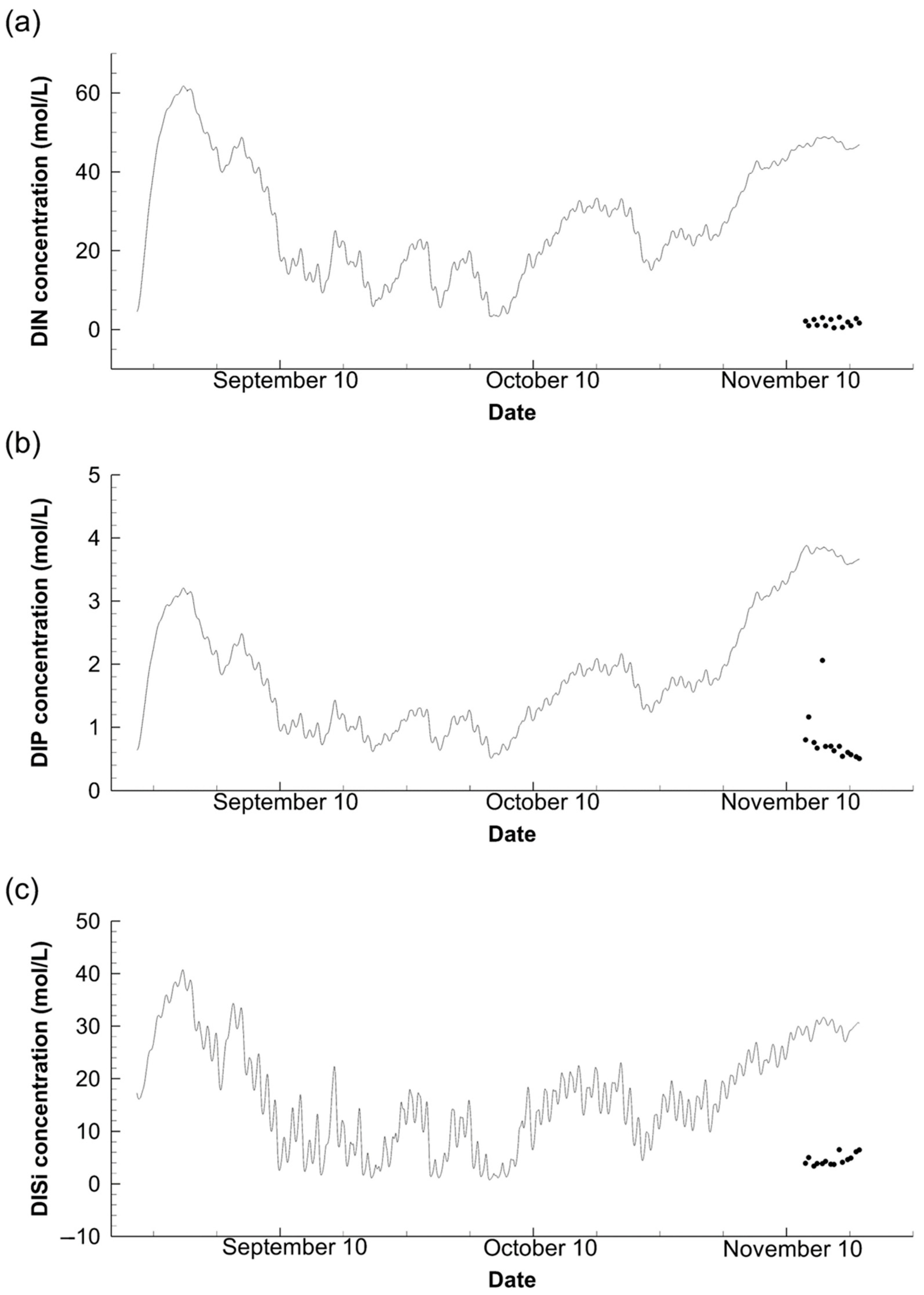
Nutrient concentration is one of the main concerns for this work because measurements were only taken twice a day and inadequately represented daily fluctuations in the pond. The above reasoning in Section 3.2 and Section 3.3 explains why it is unsurprising that there were substantial daily fluctuations in nutrients. Typically, the stratification disappearance caused the most fluctuation (e.g., Figure 7c). Three nutrients generally exhibited identical fluctuation patterns, while the concentration of dissolved nitrogen outweighed the others. This demonstrates the relative advantageous amount of nitrogen absorption by phytoplankton, showing consistency with the previous analysis [14]. Three nutrients had been at low concentrations for almost a month, but from mid-October, their concentrations have been rising, which was directly affected by the phytoplankton fluctuation (Figure 6). The subsequent fluctuation in all nutrients exactly corresponded to the phytoplankton shrinkage. The comparison period might reveal that the phosphorus concentration was the best calculated, with a minimum deviation value if calculated statistically. However, when considering the measurement precision and relatively low concentration of dissolved phosphorus, the numerical accuracy was comparable among three nutrients, and all concentrations were somewhat higher than their observation. This discrepancy is consistent with the previous study [14], where the complex relationship related to the nitrogen concentration of the pond was proposed as the explanation.
3.4. Sludge Accumulation
The accumulation of sludge is another significant concern for this work, as the sedimental condition is crucial for shrimp aquaculture ponds [5,6,13]. Although the current model is unable to evaluate sludge accumulation directly, the carbon weight of anaerobic organic matter qualitatively displays the sludge condition in the pond (Figure 8). The observed accumulation was concentrated in the middle and right bottom of the pond, which was consistent with the simulated results. Also, anaerobic organic matter was found in considerable concentrations in the side pond, which is partially affected by the numerical accuracy of flow pattern. From this perspective, the main characteristics of the sludge accumulation have been represented by the simulation results. The horizontal distribution of the sludge accumulation, however, is the simulation results’ greatest merit because it is difficult to accurately quantify the actual distribution of sludge accumulation based on the experience of local employees. The calculation results suggest that a clean zone may be found near the paddle-wheel aerators (Figure 8b), due to the high-speed flow. Furthermore, the sludge was distributed asymmetrically, with the upper side being relatively clean—a characteristic that might be attributed to the topography of the pond.
3.5. Future Research Priorities on Management
Recent research has emphasized the prioritization of operational aspects, with studies predominantly focusing on evaluating the development of intensive shrimp farming in land-based ponds, particularly in terms of production and management [33]. These investigations have consistently shown that high-density shrimp ponds exhibit a higher prevalence of heterotrophic bacteria, elevated levels of suspended particulate matter, and increased abundances of phytoplankton as observed in our target pond [34]. Consequently, they advocated for providing sufficient feed to mitigate the risk of farming failure. However, other studies suggested that cultivated shrimp may not efficiently utilize additional feed during the late stage, influenced by the dynamics of the benthic food web in ponds, potentially leading to overfeeding and degradation of the benthic environment [35]. Research comparing four widely used pond bottom treatments indicated that a cost-effective and ecologically beneficial approach involves combining natural dry-out with liming and frequent sediment removal [36]. These findings aligned with those of bio-economic modeling, demonstrating that enhanced economic profitability is associated with a shorter aquaculture period and quicker rotation [37].
As of the time of writing, the prevailing trend seems to be the adoption of autonomous monitoring systems, providing more comprehensive real-time information and facilitating further analysis [38]. Nevertheless, through this work, our understanding of shrimp aquaculture ponds has been augmented by upgrading the spatial dimension of ecosystem modeling. From this perspective, we recommend that future research efforts should include the development and utilization of three-dimensional modeling.
4. Conclusions
This study presents an evaluation of the ecosystem environment of a shrimp aquaculture pond in Kyushu District, Japan. Although the pond was the focus of a previous study, we have upgraded the model to a three-dimensional hydrodynamic environment. These simulation results demonstrated a high degree of accuracy when compared to the observation data; only little variations were confirmed when compared to the findings of the previous study. The comparison shows that our attempt to the three-dimensional environment is successful, with the following two main findings.
First, the intensive shrimp aquaculture in the targeted pond created a unique ecosystem. It was a shallow pond with a relatively high density of farmed shrimp, resulting in the concentration of chlorophyll a in it to be 100 times greater than in the adjacent outer marine environment. Despite this, our results initially showed how stratification impacted the pond ecosystem and confirmed the significant daily fluctuations in the water quality since stratification disappeared. More importantly, the horizontal distribution of anaerobic organic matter qualitatively indicated the accumulation of sludge, which assists the manual cleaning of anoxic sediments and reduces the risk associated with shrimp aquaculture.
Second, although the three-dimensional simulation has advanced the general understanding of the environment in shrimp ponds, the accuracy remains unsolved regarding sudden environmental fluctuations. There has been a noticeable drop in the dissolved oxygen concentration, but the calculation has not been successful. This discrepancy is plausibly a result of shrimp activities, and it meanwhile raises the risk of shrimp aquaculture. When necessary, a shrimp growth model could be coupled to narrow the difference in the future.
Overall, this study contributes to the sustainable management of intensive shrimp aquaculture because the developed model will be useful to determine the optimal number and the location of paddle wheel aerators to minimize energy consumed. Furthermore, this study identifies future research priorities for improving environmental assessments and operations.
Author Contributions
Conceptualization, J.Z., T.T. and D.K.; methodology, J.Z. and T.T.; software, J.Z. and T.T.; validation, J.Z., T.T. and H.W.; formal analysis, J.Z., T.T. and D.K.; investigation, D.K.; data curation, J.Z. and D.K.; writing—original draft preparation, J.Z.; writing—review and editing, J.Z., T.T., H.W. and D.K.; visualization, J.Z. and T.T.; supervision, D.K.; project administration, D.K. All authors have read and agreed to the published version of the manuscript.
Funding
This research received no external funding.
Institutional Review Board Statement
Not applicable.
Informed Consent Statement
Not applicable.
Data Availability Statement
All data included in this study are available upon request by contact with the corresponding author.
Acknowledgments
We received assistance from N. Yamayoshi, a master course student at the time, in conducting field survey. The authors would like to express their deepest gratitude to Takusui Co., Ltd., Japan, for their cooperation on the field investigation.
Conflicts of Interest
The authors declare no conflicts of interest.
References
- Steinmetz, G. This Mind-Bending Drone Footage Shows the Scale of the World’s Largest Shrimp Farm. Available online: https://businessinsider.com/video-shows-scale-of-the-world-largest-shrimp-farm-2017-2 (accessed on 27 January 2024).
- Ottinger, M.; Clauss, K.; Kuenzer, C. Large-Scale assessment of coastal aquaculture ponds with Sentinel-1 time series data. Remote Sens. 2017, 9, 440. [Google Scholar] [CrossRef]
- Shang, Y.C.; Leung, P.; Ling, B.H. Comparative economics of shrimp farming in Asia. Aquaculture 1998, 164, 183–200. [Google Scholar] [CrossRef]
- Páez-Osuna, F. The Environmental impact of shrimp aquaculture: Causes, effects, and mitigating alternatives. Environ. Manag. 2001, 28, 131–140. [Google Scholar] [CrossRef]
- Chevakidagarn, P.; Danteravanich, S. Environmental impact of white shrimp culture during 2012–2013 at Bandon Bay, Surat Thani Province: A case study investigating farm size. Agric. Nat. Resour. 2017, 51, 109–116. [Google Scholar] [CrossRef]
- Wang, J.K. Managing shrimp pond water to reduce discharge problems. Aquac. Eng. 1990, 9, 61–73. [Google Scholar] [CrossRef]
- Tacon, A.G.J. Nutritional studies in crustaceans and the problems of applying research findings to practical farming systems. Aquac. Nutr. 1996, 2, 165–174. [Google Scholar] [CrossRef]
- Burford, M.A.; Jackson, C.J.; Preston, N.P. Reducing nitrogen waste from shrimp farming: An integrated approach. In The New Wave: Proceedings of the Special Session on Sustainable Shrimp Culture; Browdy, C.L., Jory, D.E., Eds.; World Aquaculture Society: Baton Rouge, LA, USA, 2001; pp. 35–43. ISBN 978-1888807059. [Google Scholar]
- Jory, D.E.; Cabrera, T.R.; Dugger, D.M.; Fegan, D.; Lee, P.G.; Lawrence, L.; Jackson, C.J.; Mcintosh, R.P.; Castañeda, J.; International, B.; et al. A global review of shrimp feed management: Status and perspectives. Aquaculture 2001, 2001, 104–152. [Google Scholar]
- Hilborn, R.; Mangel, M. The Ecological Detective: Confronting Models with Data; Princeton University Press: Princeton, NJ, USA, 1997. [Google Scholar]
- Lorenzen, K.; Struve, J.; Cowan, V.J. Impact of farming intensity and water management on nitrogen dynamics in intensive pond culture: A mathematical model applied to Thai commercial shrimp farms. Aquac. Res. 1997, 28, 493–507. [Google Scholar] [CrossRef]
- Burford, M.A.; Costanzo, S.D.; Dennison, W.C.; Jackson, C.J.; Jones, A.B.; McKinnon, A.D.; Preston, N.P.; Trott, L.A. A synthesis of dominant ecological processes in intensive shrimp ponds and adjacent coastal environments in NE Australia. Mar. Pollut. Bull. 2003, 46, 1456–1469. [Google Scholar] [CrossRef]
- Burford, M.A.; Lorenzen, K. Modeling nitrogen dynamics in intensive shrimp ponds: The role of sediment remineralization. Aquaculture 2004, 229, 129–145. [Google Scholar] [CrossRef]
- Kitazawa, D.; Hakuta, K.; Yamayoshi, N.; Tabeta, S. Field measurement and modelling of the material cycle in the cultivation pond of penaeid shrimp Penaeus japonicus. In Proceedings of the ASME 2007 26th International Conference on Offshore Mechanics and Arctic Engineering (OMAE), San Diego, CA, USA, 10–15 June 2007; pp. 53–60. [Google Scholar] [CrossRef]
- Peterson, E.L.; Walker, M.B. Effect of speed on Taiwanese paddlewheel aeration. Aquac. Eng. 2002, 26, 129–147. [Google Scholar] [CrossRef]
- Kang, Y.H.; Lee, M.O.; Choi, S.D.; Sin, Y.S. 2-D Hydrodynamic model simulating paddlewheel-driven circulation in rectangular shrimp culture ponds. Aquaculture 2004, 231, 163–179. [Google Scholar] [CrossRef]
- Kittiwanich, J.; Songsangjinda, P.; Yamamoto, T.; Fukami, K.; Muanagyao, P. Modeling the effect of nitrogen input from feed on the nitrogen dynamics in an enclosed intensive culture pond of black tiger shrimp (Penaeus monodon). Coas. Mar. Sci. 2012, 35, 39–51. [Google Scholar]
- Poersch, L.H.; Milach, Â.M.; Cavalli, R.O.; Wasielesky, W.J.R.; Möller, O.; Castello, J.P. Use of a mathematical model to estimate the impact of shrimp pen culture at Patos Lagoon Estuary, Brazil. An. Acad. Bras. Ciênc. 2014, 86, 1063–1076. [Google Scholar] [CrossRef] [PubMed]
- Mirzaei, F.S.; Ghorbani, R.; Hosseini, S.A.; Haghighi, F.P.; Saravi, H.N. Associations between shrimp farming and nitrogen dynamic: A model in the Caspian Sea. Aquaculture 2019, 510, 323–328. [Google Scholar] [CrossRef]
- Soriano, F.A.C.; Junquera, V.I.; Minakata, P.E.; Cano, O.M.; Paz, J.d.J.O.; Ramirez, J.C.A.; Willerer, A.O.M. Nitrogen dynamics model in zero water exchange, low salinity intensive ponds of white shrimp, Litopenaeus vannamei, at Colima, Mexico. Lat. Am. J. Aquat. Res. 2013, 41, 68–79. [Google Scholar] [CrossRef]
- Silfiana; Widowati; Putro, S.P.; Udjiani, T. Modeling of nitrogen transformation in an integrated multi-trophic aquaculture (IMTA). J. Phys. Conf. Ser. 2018, 983, 12122. [Google Scholar] [CrossRef]
- Widowati; Putro, S.P.; Silfiana. Stability analysis of the phytoplankton effect model on changes in nitrogen concentration on integrated multi-trophic aquaculture systems. J. Phys. Conf. Ser. 2018, 1025, 12088. [Google Scholar] [CrossRef]
- Araneda, M.E.; Hernández, J.M.; Gasca-Leyva, E.; Vela, M.A. Growth modelling including size heterogeneity: Application to the intensive culture of white shrimp (P. vannamei) in freshwater. Aquac. Eng. 2013, 56, 1–12. [Google Scholar] [CrossRef]
- de Melo Filho, M.E.S.; Owatari, M.S.; Mouriño, J.L.P.; Carciofi, B.A.M.; Soares, H.M. Empirical modeling of feed conversion in pacific white shrimp (Litopenaeus vannamei) growth. Ecol. Model. 2020, 437, 109291. [Google Scholar] [CrossRef]
- Dong, S.; Liu, D.; Zhu, B.; Yu, L.; Shan, H.; Wang, F. A dynamic energy budget model for kuruma shrimp Penaeus japonicus: Parameterization and application in integrated marine pond aquaculture. Animals 2022, 12, 1828. [Google Scholar] [CrossRef] [PubMed]
- Zarzar, C.A.; Fernandes, T.J.; Cardoso de Oliveira, I.R. Modeling the growth of pacific white shrimp (Litopenaeus vannamei) using the new Bayesian hierarchical approach based on correcting bias caused by incomplete or limited data. Ecol. Inform. 2023, 77, 102271. [Google Scholar] [CrossRef]
- Lin, Q.; Yang, W.; Zheng, C.; Lu, K.; Zheng, Z.; Wang, J.; Zhu, J. Deep-learning based approach for forecast of water quality in intensive shrimp culture ponds. Indian J. Fish. 2018, 65, 75–80. [Google Scholar] [CrossRef]
- Ma, Z.; Song, X.; Wan, R.; Gao, L.; Jiang, D. Artificial neural network modeling of the water quality in intensive Litopenaeus vannamei shrimp tanks. Aquaculture 2014, 433, 307–312. [Google Scholar] [CrossRef]
- Ahmad, T.; Boyd, C.E. Design and peroormance of paddle wheel aerators. Aquac. Eng. 1988, 7, 39–62. [Google Scholar] [CrossRef]
- Chatvijitkul, S.; Boyd, C.E.; Davis, D.A. Nitrogen, phosphorus, and carbon concentrations in some common aquaculture feeds. J. World Aquac. Soc. 2017, 49, 477–483. [Google Scholar] [CrossRef]
- Ginot, V.; Hervé, J.-C. Estimating the parameters of dissolved oxygen dynamics in shallow ponds. Ecol. Modell. 1994, 73, 169–187. [Google Scholar] [CrossRef]
- Marques, G.M.; Augustine, S.; Lika, K.; Pecquerie, L.; Domingos, T.; Kooijman, S.A.L.M. The AmP project: Comparing species on the basis of dynamic energy budget parameters. PLoS Comput. Biol. 2018, 14, e1006100. [Google Scholar] [CrossRef] [PubMed]
- Junda, M. Development of intensive shrimp farming, Litopenaeus vannamei in land-based ponds: Production and management. J. Phys. Conf. Ser. 2018, 1028, 012020. [Google Scholar] [CrossRef]
- Alfiansah, Y.R.; Hassenrück, C.; Kunzmann, A.; Taslihan, A.; Harder, J.; Gärdes, A. Bacterial abundance and community composition in pond water from shrimp aquaculture systems with different stocking densities. Front. Microbiol. 2018, 9, 2457. [Google Scholar] [CrossRef]
- Huang, Q.; Olenin, S.; Li, L.; Sun, S.; De Troch, M. Meiobenthos as food for farmed shrimps in the earthen ponds: Implications for sustainable feeding. Aquaculture 2020, 521, 735094. [Google Scholar] [CrossRef]
- Yuvanatemiya, V.; Boyd, C.E.; Thavipoke, P. Pond bottom management at commercial shrimp farms in Chantaburi Province, Thailand. J. World Aquac. Soc. 2011, 42, 618–632. [Google Scholar] [CrossRef]
- Shinji, J.; Nohara, S.; Yagi, N.; Wilder, M. Bio-economic analysis of super-intensive closed shrimp farming and improvement of management plans: A case study in Japan. Fish. Sci. 2019, 85, 1055–1065. [Google Scholar] [CrossRef]
- Wardhany, V.A.; Yuliandoko, H.; Subono; Harun, A.M.U.; Astawa, I.G.P. Smart system and monitoring of Vanammei shrimp ponds. Int. J. Adv. Sci. Eng. Inf. Technol. 2021, 11, 1366. [Google Scholar] [CrossRef]
Figure 1.
Locations of Kyushu District, Japan, and shrimp aquaculture pond (a) monitoring sites (blue points) and two paddle-wheel aerators (red points) in the pond (b). The pipes of inflow and outflow of water were installed at Stations A and B, respectively. The intake pipe was drawn from the outer sea (Station D).
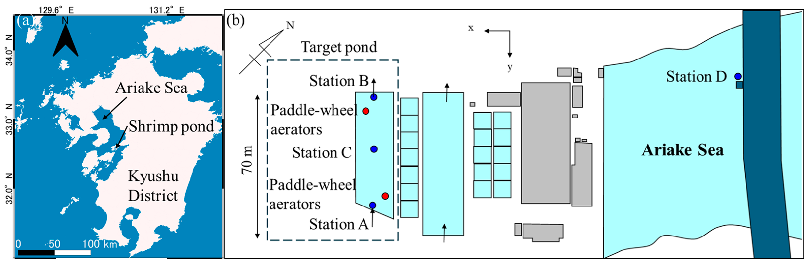
Figure 2.
The grid system for simulation and the locations of monitoring (validation) stations (in blue) and paddle-wheel aerators (in red) (a) and the vertical velocity profile given at the grid of paddle-wheel aerators (b). The gray grids in (a) represent the land.
Figure 2.
The grid system for simulation and the locations of monitoring (validation) stations (in blue) and paddle-wheel aerators (in red) (a) and the vertical velocity profile given at the grid of paddle-wheel aerators (b). The gray grids in (a) represent the land.
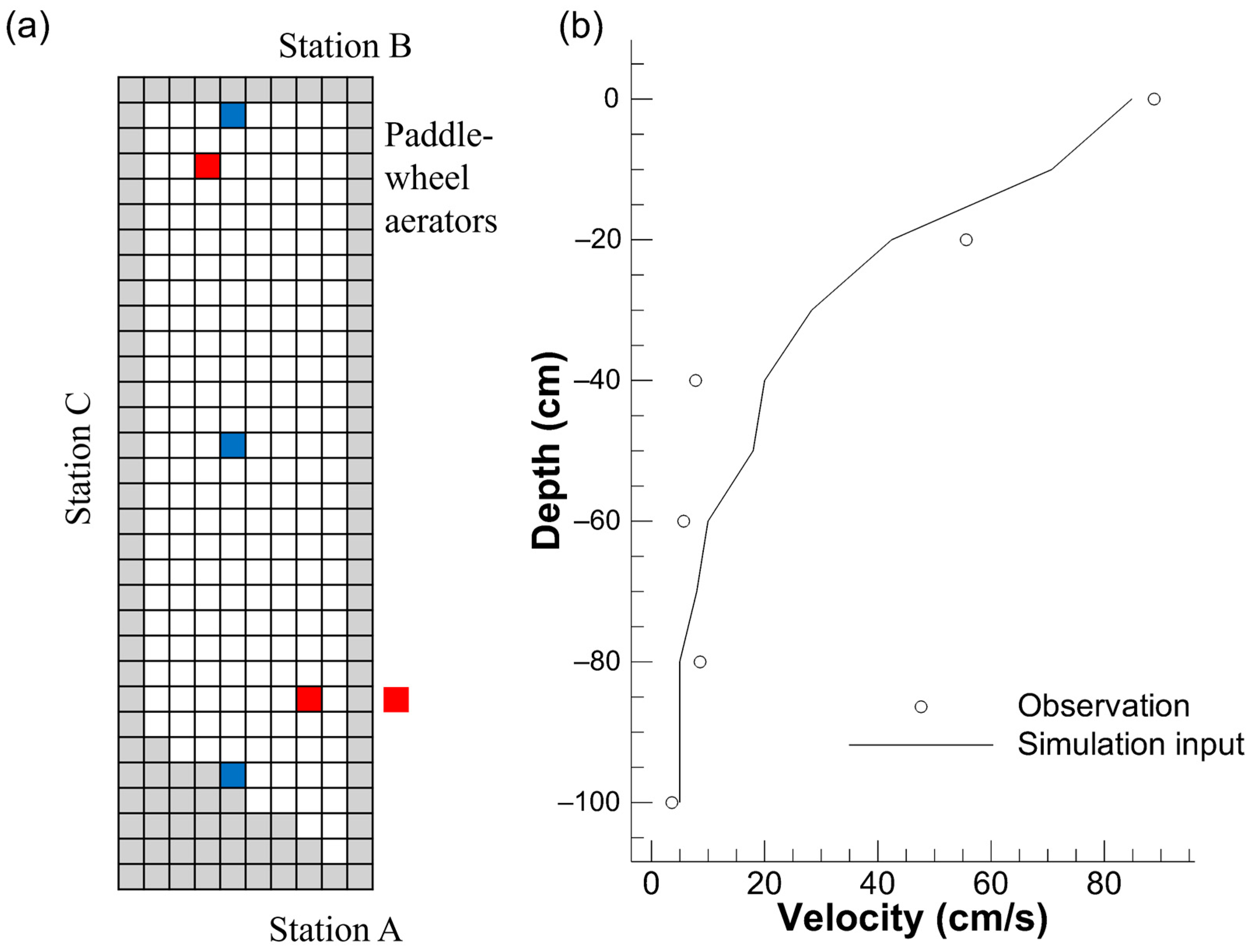
Figure 3.
Comparison of the observational (a) and numerical (b) flow pattern on 3 November 2006. The arrows represent the magnitude and direction of velocities. Note the slight discrepancy in the pond’s left bottom corner caused by the numerical simplification of the topography.
Figure 3.
Comparison of the observational (a) and numerical (b) flow pattern on 3 November 2006. The arrows represent the magnitude and direction of velocities. Note the slight discrepancy in the pond’s left bottom corner caused by the numerical simplification of the topography.

Figure 4.
Comparison of the observational (points) and numerical (line) water temperature at 40 cm below the water surface of Station C throughout the simulation period.
Figure 4.
Comparison of the observational (points) and numerical (line) water temperature at 40 cm below the water surface of Station C throughout the simulation period.
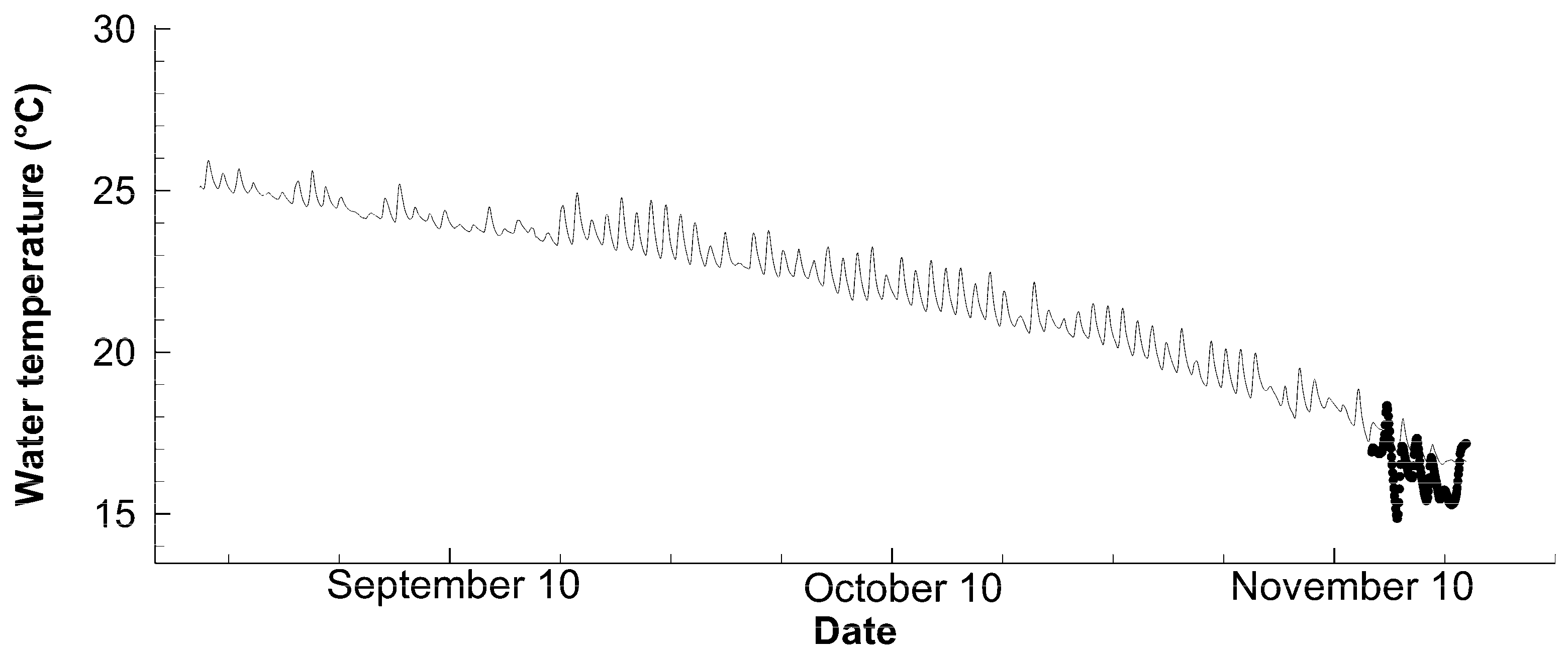
Figure 5.
Comparison of the observational (points) and numerical (line) chlorophyll a concentration, at 40 cm below the water surface of Station C throughout the simulation period.
Figure 5.
Comparison of the observational (points) and numerical (line) chlorophyll a concentration, at 40 cm below the water surface of Station C throughout the simulation period.

Figure 6.
Comparison of the observational (points) and numerical (line) dissolved oxygen concentration at 80 cm below the water surface of Station C throughout the simulation period.
Figure 6.
Comparison of the observational (points) and numerical (line) dissolved oxygen concentration at 80 cm below the water surface of Station C throughout the simulation period.
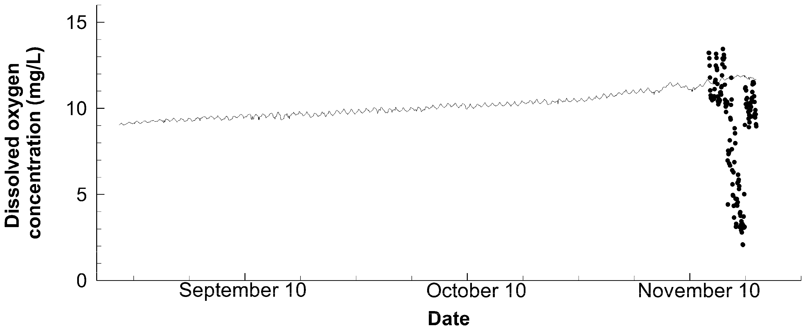
Figure 7.
Comparison of the observational (points) and numerical (line) for dissolved inorganic nitrogen (DIN); (a) phosphorus (DIP) (b) and silicon (DISi) (c), at water surface of Station B throughout the simulation period.
Figure 7.
Comparison of the observational (points) and numerical (line) for dissolved inorganic nitrogen (DIN); (a) phosphorus (DIP) (b) and silicon (DISi) (c), at water surface of Station B throughout the simulation period.

Figure 8.
Comparison of the observational (a) and numerical (b) for the sludge accumulation at the bottom of the shrimp pond during the aquaculture period. The carbon weight of anaerobic organic matter has been taken as the numerical alternative for the sludge accumulation. The white circles represent the paddle-wheel aerators.


Table 1.
A summarized condition of water quality monitoring.
| Items | Instrument | Setup |
|---|---|---|
| Water temperature | Compact-CT | Every 30 min values at 40 cm below the water surface of Station C |
| Chlorophyll a | Compact-CLW | Every 10 min values at 40 cm below the water surface of Station C |
| Dissolved oxygen | Compact-DOW | Every 10 min values at 80 cm below the water surface of Station C |
| Nutrient | Water samples | 50 mL each at 6:00 and 15:00 every day from the drawing pipe at Station A and from the surface water at Station B |
| Water treatment and analysis | immediately frozen in the refrigerator before the laboratory; filtered using a Whatman GF/F glass filter paper and analyzed by the Auto Analyzer in the laboratory |
Disclaimer/Publisher’s Note: The statements, opinions and data contained in all publications are solely those of the individual author(s) and contributor(s) and not of MDPI and/or the editor(s). MDPI and/or the editor(s) disclaim responsibility for any injury to people or property resulting from any ideas, methods, instructions or products referred to in the content. |
© 2024 by the authors. Licensee MDPI, Basel, Switzerland. This article is an open access article distributed under the terms and conditions of the Creative Commons Attribution (CC BY) license (https://creativecommons.org/licenses/by/4.0/).
Share and Cite
MDPI and ACS Style
Zhou, J.; Tu, T.; Wang, H.; Kitazawa, D. Modeling Environmental Impacts of Intensive Shrimp Aquaculture: A Three-Dimensional Hydrodynamic Ecosystem Approach. Fishes 2024, 9, 126. https://doi.org/10.3390/fishes9040126
AMA Style
Zhou J, Tu T, Wang H, Kitazawa D. Modeling Environmental Impacts of Intensive Shrimp Aquaculture: A Three-Dimensional Hydrodynamic Ecosystem Approach. Fishes. 2024; 9(4):126. https://doi.org/10.3390/fishes9040126
Chicago/Turabian StyleZhou, Jinxin, Teng Tu, Huajin Wang, and Daisuke Kitazawa. 2024. "Modeling Environmental Impacts of Intensive Shrimp Aquaculture: A Three-Dimensional Hydrodynamic Ecosystem Approach" Fishes 9, no. 4: 126. https://doi.org/10.3390/fishes9040126