Negative Energy Antiferromagnetic Instantons Forming Cooper-Pairing ‘Glue’ and ‘Hidden Order’ in High-Tc Cuprates

Abstract

An emergence of magnetic boson of instantonic nature, that provides a Cooper-‘pairing glue’, is considered in the repulsive ‘nested’ Hubbard model of superconducting cuprates. It is demonstrated that antiferromagnetic instantons of a spin density wave type may have negative energy due to coupling with Cooper pair condensate. A set of Eliashberg like equations is derived and solved self-consistently, proving the above suggestion. An instantonic propagator plays the role of the Green function of the pairing ‘glue’ boson. Simultaneously, the instantons defy condensation of the mean-field spin-density wave (SDW) order. We had previously demonstrated in analytical form that periodic chain of instanton-anti-instanton pairs along the axis of Matsubara time has zero scattering cross section for weakly perturbing external probes, like neutrons, etc., thus representing a ‘hidden order’. Hence, the two competing orders, superconducting and antiferromagnetic, may coexist (below some $T_c$) in the form of the superconducting order coupled to ‘hidden’ instantonic one. This new picture is discussed in relation with the mechanism of high temperature superconductivity.

1. Introduction

We present here an idea of instanton-mediated superconductivity using a ‘minimal’ model Hamiltoninan of electronic system with spin-fermion coupling [1,2] to a bosonic mode on a square lattice with antiferromagnetic (AF) wave vector $\overrightarrow{Q}$ near the ‘nested’ Fermi-surface points in momentum space. It proves to be that this simple model incorporates intrinsic creation of instantons and provides a unified explanation of an emergence of a ‘hidden order’ state followed by a transition to superconductivity. To explain a matter of principle we consider here just a model of fermions on a square lattice linearly coupled to a spin subsystem with dominating AF spin fluctuations. The latter are described by effective nonlinear Euclidean action $S_s$:

$$S={\int }_0^{\beta }d\tau \left[\sum _{i,\sigma }{c}_{i\sigma }^{+}({\partial }_{\tau }-{\mu }_e)c_{i\sigma }-\sum _{i,j,\sigma }{t}_{ij}{c}_{i\sigma }^{+}{c}_{j\sigma }+\sum _{i,\sigma ,{\sigma }^{\prime }}{c}_{i\sigma }^{+}{\overrightarrow{S}}_i\cdot {\overrightarrow{\sigma }}_{\sigma {\sigma }^{\prime }}{c}_{i{\sigma }^{\prime }}\right]+S_s;$$

(1)

$$S_s={\int }_0^{\beta }d\tau \left[\sum _i{\left({\partial }_{\tau }{\overrightarrow{S}}_i\right)}^2+\sum _{i,j}{J}_{ij}{\overrightarrow{S}}_i\cdot {\overrightarrow{S}}_j+\sum _{i}V\left({\overrightarrow{S}}_i\right)\right].$$

(2)

where $\overrightarrow{\sigma }=\left\{{\sigma }_x,{\sigma }_y,{\sigma }_z\right\}$ are the Pauli matrices, and ${\mu }_e$ is the chemical potential. This model could be considered formally as being an effective infrared-scale theory obtained by a proper renormalisation of the Hubbard-like on-site repulsive-U Hamiltonian [3,4]. In principle, two-component spin-fermion models could be derived from taking into account details of Cu and O orbitals in cuprates [5,6]. Naively, one would expect the spin subsystem part $S_s$ to consist just of the Hubbard-Stratonovich ‘spin-field’ quadratic term $\frac{3}{2U}{\sum }_i{\left(\overrightarrow{S}\right)}^2$ (cast into general $V\left({\overrightarrow{S}}_i\right)$ term in (2)), that together with the spin-fermion term ${\sum }_{i,\sigma ,{\sigma }^{\prime }}{c}_{i\sigma }^{+}{\overrightarrow{S}}_i\cdot {\overrightarrow{\sigma }}_{\sigma {\sigma }^{\prime }}{c}_{i{\sigma }^{\prime }}$, restores the familiar onsite repulsion, $\propto U{\sum }_i{n}_{i\uparrow }{n}_{i\downarrow }$, of the Hubbard-U model after path integration over spins ${\overrightarrow{S}}_i\left(\tau \right)$, where $n_{i\sigma }=c_{i\sigma }^{+}{c}_{i\sigma }$. But, in reality, one has also to allow for the spin-exchange terms of the kind ${\sum }_{i,j}{J}_{ij}{\overrightarrow{S}}_i\cdot {\overrightarrow{S}}_j$, that are generated by inter-site fermionic (indirect) exchange, and cause spin dynamics, creating the AF spin ordering fluctuations. The quartic and higher order in ${\overrightarrow{S}}_i$ terms are cast into $V\left({\overrightarrow{S}}_i\right)$ term in (2) as well, compare [7]. To proceed, we single out the most important for the rest part of the spin-fermion system action, that follows from the general expressions (1) and (2) and is conveniently written in the Fourier representation, assuming summation over the momenta in 2D Brillouin zone of the square lattice:

$$\begin{array}{c}\tilde{S}={\int }_0^{\beta }d\tau \left[\sum _{\mathbf{q},s}{c}_{\mathbf{q}\mathbf{s}}^{+}({\partial }_{\tau }+{\epsilon }_q)c_{\mathbf{q},s}+\sum _{\mathbf{q},\mathbf{Q},s,s^{\prime }}\left(c_{\mathbf{q}+\mathbf{Q},s}^{+}{\overrightarrow{S}}_{\mathbf{Q}}\left(\tau \right)\cdot {\overrightarrow{\sigma }}_{s{s}^{\prime }}{c}_{\mathbf{q},s^{\prime }}+H.c.\right)+\right.\hfill \\ \left.\sum _{\mathbf{Q}}\left({\partial }_{\tau }{\overrightarrow{S}}_{\mathbf{Q}}\cdot {\partial }_{\tau }{\overrightarrow{S}}_{-\mathbf{Q}}+v_s^2{(\mathbf{Q}-{\mathbf{Q}}_{AF})}^2|{\overrightarrow{S}}_{\mathbf{Q}}{|}^2+{\mu }_0{|{\overrightarrow{S}}_{\mathbf{Q}}|}^2\right)+\lambda \sum _{\mathbf{Q},{\mathbf{Q}}^{\prime }}|{\overrightarrow{S}}_{\mathbf{Q}}{|}^2\cdot {|{\overrightarrow{S}}_{{\mathbf{Q}}^{\prime }}|}^2\right]\hfill \end{array}$$

(3)

where we have introduced the AF wave vector ${\mathbf{Q}}_{AF}=\{\pi ,\pi \}$ expressed in the inverse units $a^{-1}$ of the square lattice, and $v_s$ is a spin-wave velocity, ${\mu }_0$ enters a ‘mass’ term, that defines finite correlation length of the AF fluctuations, $\lambda$ characterises coupling between the different spin fluctuations, and ${\epsilon }_q$ is fermionic dispersion shifted by the chemical potential ${\mu }_e$.

Leaving for the future work a solution of the 2+1D Higgs model that stems from the symmetries of the Euclidean action in (3) [7,8], we consider here much simplified version, that nevertheless demonstrates our major idea of the condensation of an instantonic Cooper-pairing ‘glue’. Namely, we introduce Ising spin $M_{\mathbf{Q}}$ instead of the Heisenberg spin ${\overrightarrow{S}}_{\mathbf{Q}}$ and, as an indulgence for the loss of the local rotational degrees of freedom, introduce a local rotation frame with the spin polarization axis changing direction on the scale of a ‘spin-bag’ size. The latter is of the order of the spin correlation length $\propto \sqrt{{{\mu }_0}^{-1}}$. Since we have introduced a local spin polarization axis in each bag e.g., aligned along the z-axis, the scalar product of the Pauli matrices and Fourier component of the spin vector in a particular ‘spin-bag’ could be substituted with the product of corresponding projections in the rotated ‘spin-bag’ reference frame: ${\overrightarrow{S}}_{\mathbf{Q}}\cdot \overrightarrow{\sigma }=M_{\mathbf{Q}}\cdot \sigma$, where $\sigma =\pm 1/2$. Simultaneously, the spin part of the fermionic field operators should be transformed with the unitary $2\times 2$ matrix $\widehat{R}(i,\tau )$: $c_{i\sigma }\to R_{i,\sigma {\sigma }^{\prime }}\cdot c_{i{\sigma }^{\prime }}$ and $c_{i\sigma }^{+}\to c_{i{\sigma }^{\prime }}^{+}{R^{†}}_{i,{\sigma }^{\prime }\sigma }$, that changes as a function of the point in the Euclidean space-time $i,\tau$. Then, the terms in (1), $c^{+}{\partial }_{\tau }c;c^{+}c$, generate dynamics of SU(2) guage field $\widehat{R}(i,\tau )$ and provide corresponding extra terms in the Euclidean action (3) [7,8]. In what follows we consider approximately complicated dynamics of the fermionic- $c^{+},c$, guage- $\widehat{R}$ and Higgs- $\overrightarrow{S}$ fields. Namely, the whole system is divided into a conglomerate of the ‘spin-bags’, their number is of the order of $N\propto V{{\mu }_0}^2>>1$, where V is 2D volume of the system. Each bag possesses space index i, now enumerating the ‘centers’ of the different bags inside the system. Each bag accommodates an antiferromagnetic spin-density wave (SDW) fluctuation, polarized along the i-th bag’s (local) spin polarization axis. The amplitude of the SDW fluctuation depends on the imaginary Matsubara time: $M_i\left(\tau \right)$, and possesses a single AF wave-vector $\overrightarrow{Q_{AF}}$. To allow for the change of the ‘spin-bag’ reference frames between the different bags we introduce the fluctuating phases ${\varphi }_i=Im\left\{log{M}_i\left(\tau \right)\right\}$, that change at random as function of the bag’s index i. Then, the Euclidean action (3) becomes:

$${\tilde{S}}_M={\int }_0^{\beta }d\tau \left[\sum _{\mathbf{q},\sigma }{c}_{\mathbf{q}\sigma }^{+}({\partial }_{\tau }+{\epsilon }_q)c_{\mathbf{q},\sigma }+\sum _{\mathbf{q},\sigma ,i}\left(c_{\mathbf{q}+{\mathbf{Q}}_{\mathit{AF}},\sigma }^{+}{M}_i\left(\tau \right)\sigma c_{\mathbf{q},\sigma }+H.c.\right)\right]+S_{sM}$$

(4)

$$S_{sM}={\int }_0^{\beta }d\tau \frac{1}{2g_{sf}{U}^2}\sum _i\left\{{\left({\partial }_{\tau }{M}_i\right)}^2+2\frac{{\mu }_0^2}{\lambda }{M_i}^2+{M_i}^4\right\}.$$

(5)

Here space distribution of spin fluctuation projection on the ith bag’s local z-axis, possessing AF wave vector ${\overrightarrow{Q}}_{AF}$, is characterized by the Matsubara time dependent complex amplitude $M_i\left(\tau \right)$:

$$M_i(\tau ,\mathbf{r})=M_i\left(\tau \right)e^{i{\mathbf{Q}}_{\mathit{AF}}\cdot \mathbf{r}}+{M_i}^{*}\left(\tau \right)e^{-i{\mathbf{Q}}_{\mathit{AF}}\cdot \mathbf{r}},M_i\left(\tau \right)\equiv |M_i|e^{i{\varphi }_i}$$

(6)

Several remarks are in order now. Comparison of (3) and (5) with (1) shows that we have approximated summation over SDW wave vector $\overrightarrow{Q}$ in the spin-fermion scattering terms with assignment of a finite weight to a single AF wave vector ${\overrightarrow{Q}}_{AF}$, assuming that this contribution dominates in the integrations in the Eliashberg like equations with the spin-fermion vertices, compare [1]. Consequently, the real-space antiferromagnetic spin rigidity energy in (3), $\propto v_s^2{(\overrightarrow{Q}-{\overrightarrow{Q}}_{AF})}^2{|{\overrightarrow{S}}_{\overrightarrow{Q}}|}^2$, is dropped in (5), as we consider only spin fluctuations with the wave vectors $\overrightarrow{Q}\approx {\overrightarrow{Q}}_{AF}$. Besides, we have chosen a local spin polarization axis in each ‘spin-bag’, thus substituting scalar product of Fourier component of the spin vector ${\overrightarrow{S}}_{\mathbf{Q}}\cdot \overrightarrow{\sigma }$ and of fermion spin operator $\overrightarrow{\sigma }$ with the product of corresponding projections in the rotated reference frame of the i-th bag [7]: ${\overrightarrow{S}}_{\mathbf{Q}}\cdot \overrightarrow{\sigma }=M_i\cdot s$. Since bosonic spin field must be $\tau$-periodic, the amplitude in (6) obeys periodicity condition:

$$\begin{array}{c}\hfill M_i\left(\tau +1/T\right)=M_i\left(\tau \right),\end{array}$$

(7)

where T is temperature, and dependence of $M_i$ on coordinate is due to periodic variation of the prefactor $\sim e^{i{\mathbf{Q}}_{\mathit{AF}}\cdot \mathit{r}}$ with AF wave vector ${\overrightarrow{Q}}_{AF}$. We have absorbed the coupling constant U in the definition of $M_i$ in the spin-fermion coupling (second) term in (4). This gives then a renormalized coupling constant: $g_{sf}\to g_{sf}{U}^2$. We shall consider below the case when mean-field SDW order is missing, though $\langle M_i\left(\tau \right)\rangle$ is ‘macroscopic’, i.e., proportional to the volume of a ‘spin-bag’. This means that a SDW in each spin-bag accommodates instanton-anti-instanton pairs, e.g., considered previously within effective $0+1D$ model [9]. Then, the following condition is obeyed:

$${\int }_0^{\beta }d\tau \langle M_i\left(\tau \right)\rangle =0$$

(8)

Hence, we call such ‘invisible SDW’ a quantum SDW (QSDW), to emphasise the absence of the static antiferromagnetic order.

Now we define expression for the partition function of the system. We take into account randomness of the phases ${\varphi }_i$ ascribed to the different ‘spin-bags’ by applying a ‘random phase approximation’, i.e., by taking average over ${\varphi }_i$ from 0 to $2\pi$ in the partition function:

$$Z=Z_f{Z}_{AF}\int Ad{\tau }_0\prod _i\int \mathcal{D}{\varphi }_i\langle \langle T_{\tau }\exp \left\{-{\int }_0^{\beta }\sum _{\mathbf{q},\sigma ,i}\left(c_{\mathbf{q}+{\mathbf{Q}}_{AF},\sigma }^{+}\left(\tau \right)M_i(\tau +{\tau }_0)\sigma c_{\mathbf{q},\sigma }\left(\tau \right)+H.c.\right)\right\}{\rangle }_{AF}{\rangle }_f$$

(9)

Here an interaction representation for the spin-fermion coupling term in Equation (4) is used [10], and Matsubara time $\tau$ ordering procedure is applied to the products of the quantum field-operators, as is indicated with the sign $T_{\tau }$. The Hibbs averaging is indicated by the angle brackets $\langle \dots \rangle$, being performed with the statistical weight provided by the noninteracting parts of the action of the magnetic $S_{sM}$ subsystem, see (5), and of the fermionic subsystem, $S_f$, that equals respectively:

$$S_f={\int }_0^{\beta }d\tau \left[\sum _{\mathbf{q},\sigma }{c}_{\mathbf{q}\sigma }^{+}({\partial }_{\tau }+{\epsilon }_q)c_{\mathbf{q}\sigma }\right]$$

(10)

In what follows, we shall consider instanton-populated ‘spin-bags’ for the reason explained below. Then, an integration over ${\tau }_0$ in the Equation (9) arises due to presence of the zero mode in each ‘spin-bag’, accompanying the instantonic saddle-point solution $M_0\left(\tau \right)$ of the magnetic subsystem [11]. A detailed description is given below, see Equation (20) and the text after it. Correspondingly, A-factor signifies Jacobian used for the integration over the zero mode of the magnetic action $S_{AF}$ [11], $A\sim \sqrt{S_{AF}^{cl}}$, where $S_{AF}^{cl}=S_{AF}\left(M_0\left(\tau \right)\right)$ is the saddle point value of the instantonic magnetic action. Integration over random phases ${\varphi }_i$ reflects existing symmetry of the spin subsystem on the scale of the ‘spin-bag’ size, as explained above. We introduce a short-hand notation for the farther convenience:

$$f\left(\tau \right)=\sum _{\mathbf{q},\sigma }{c}_{\mathbf{q}+{\mathbf{Q}}_{AF}\sigma }^{+}\left(\tau \right)\sigma c_{\mathbf{q}\sigma }\left(\tau \right);f^{†}\left(\tau \right)=\sum _{\mathbf{q},\sigma }{c}_{\mathbf{q}\sigma }^{+}\left(\tau \right)\sigma c{\left(\tau \right)}_{\mathbf{q}+{\mathbf{Q}}_{AF}\sigma }$$

(11)

Now, the time ordering $T_{\tau }$ permits us to rewrite (9) in the form of series expansion:

$$\begin{array}{c}Z=Z_f{Z}_{AF}\int Ad{\tau }_0\prod _j\int \mathcal{D}{\varphi }_j\sum _{n,m}{\displaystyle \frac{{(-1)}^{n+m}}{n!m!}}\langle \langle \prod _{i,k=1}^n\prod _{i^{\prime },k^{\prime }=1}^m{\int }_0^{\beta }d{\tau }_k{\int }_0^{\beta }d{\tau }_{k^{\prime }}^{\prime }{T}_{\tau }f\left({\tau }_k\right)f^{†}\left({\tau }_{k^{\prime }}^{\prime }\right){\rangle }_f\times \hfill \\ M_i({\tau }_k+{\tau }_0)M_{i^{\prime }}^{*}({\tau }_{k^{\prime }}^{\prime }+{\tau }_0){\rangle }_{AF}\hfill \end{array}$$

(12)

Independent averaging over the phases ${\varphi }_j$ of the QSDW in the different ‘spin-bags’ gives nonzero result under the conditions $n=m$ and, simultaneously, couples into “Wick-like” pairwise products the amplitudes $\left\{M_i\right\}$: $M_i({\tau }_k+{\tau }_0)M_{i^{\prime }}({\tau }_{k^{\prime }}^{\prime }+{\tau }_0){\delta }_{i,i^{\prime }}$, where ${\delta }_{ij}$ is Kronecker delta. Hence, partition function (9) reduces to:

$$\begin{array}{c}Z=Z_f{Z}_{AF}\int Ad{\tau }_0\langle \langle T_{\tau }\exp \left\{-{\int }_0^{\beta }{{\int }_0}^{\beta }d\tau d{\tau }^{\prime }\sum _{\mathbf{q},{\mathbf{q}}^{\prime },\sigma ,{\sigma }^{\prime },i}{D}_i(\tau +{\tau }_0,{\tau }^{\prime }+{\tau }_0)\sigma {\sigma }^{\prime }{c}_{\mathbf{q}+{\mathbf{Q}}_{AF},\sigma }^{+}\left(\tau \right)c_{\mathbf{q},\sigma }\left(\tau \right)\times \right.\hfill \\ \left.c_{{\mathbf{q}}^{\prime },{\sigma }^{\prime }}^{+}\left({\tau }^{\prime }\right)c_{{\mathbf{q}}^{\prime }+{\mathbf{Q}}_{AF},\sigma }\left({\tau }^{\prime }\right)\right\}{\rangle }_{AF}{\rangle }_f;D_i(\tau +{\tau }_0,{\tau }^{\prime }+{\tau }_0)=T_{\tau }{M}_i(\tau +{\tau }_0)M_i({\tau }^{\prime }+{\tau }_0)\hfill \end{array}$$

(13)

where all $M_i$ are now real. In the saddle-point approximation we substitute retarded interaction $D_i(\tau +{\tau }_0,{\tau }^{\prime }+{\tau }_0)$ in the four-fermion interaction term in (13) by the instantonic propagator $𝒟(\tau -{\tau }^{\prime })\propto \int d{\tau }_0{M}_0(\tau +{\tau }_0)M_0({\tau }^{\prime }+{\tau }_0)$ defined below in Equation (25). Hence, we have derived effective retarded interaction between the fermions inside a ‘spin-bag’, mediated by the fluctuating QSDW.

Namely, we demonstrate that, under a strong enough spin-fermion coupling in the Hamiltonian (4), a positive bare pre-factor ${\mu }_0^2$ in front of $M_i^2$ in (5) is renormalised and may become negative: $-{\mu }^2$. An intrinsic mechanism of this sign reversal, that happens below a temperature $T^{*}$, is a first order transition into a phase, that possesses a new saddle point of the Euclidean action of the Fermi-system. The saddle point accommodates a complex macroscopic fluctuation, that constitutes quantum antiferromagnetic ‘hidden’ order (QSDW) bound to a Cooper-pair condensate inside each ‘spin-bag’. We show that as the temperature T is lowered within the temperature interval $T^{*}<T<T_c$, the energy of this fluctuation crosses zero and becomes negative below $T_c$. This happens due to a growth of the amplitude of the antiferromagnetic QSDW, which is periodically modulated in the imaginary Matsubara time and has zero mean.The latter property makes this QSDW a ‘hidden order’ [9]. The periodic modulation of the QSDW amplitude along the Matsubara time axis is facilitated via sequence of (anti)instantons, an “instantonic crystal”, giving rise to instanton-mediated Cooper-pairing ‘glue’. The strength of the ‘glue’ increases as the temperature decreases, and the energy of the collective fluctuation passes through zero at $T_c$. Below $T_c$ Cooper-pairing fluctuation turns into equilibrium superconducting condensate, and the amplitude of the instantonic modulation of QSDW $M_0$ saturates and remains finite in the $T\to 0$ limit. A clip-representation of the quint essence of this scenario is presented in Figure 1. In the next section we remind derivation [9,12,13] of the zero mode instantonic propagator for an ad hoc Lagrangian of the type (5), but with sign-changed coefficient ${\mu }_0^2\to -{\mu }^2<0$, (14). The ‘hidden order’ behaviour of the QSDW characterized with this propagator is described. Next, in Section 3 we use the instantonic propagator of Section 2 as a ‘glue boson’ in the Eliashberg like system of equations, which is derived in the random-phase ${\varphi }_i=Im\left\{log{M}_i\left(\tau \right)\right\}$ approximation, and find analytic solution for the temperature Green’s functions of the Cooper-paired fermions, using a toy model in Equation (4), with dispersion ${\epsilon }_q$ possessing “nested” Fermi-surface regions. In Section 4 a negative shift of the bare coefficient ${\mu }_0^2$ is calculated explicitly via a second order variational derivative of the free energy decrease, $\Delta \Omega$, due to superconducting fluctuations: ${\delta }^2\Delta \Omega /\delta M^2\left(\tau \right)$. As a result, an algebraic self-consistency equation for the coefficient $-{\mu }^2<0$ is obtained and solved. Below a temperature $T^{*}$ this coefficient first becomes negative, which manifests transition of the Fermi-system into a state with saddle-point fluctuation described as ‘hidden order’ inside of each ‘spin-bag’ accommodating an antiferromagnetic QSDW coupled to superconducting condensate. At strong enough spin-fermion coupling the $T^{*}$ is greater than $T_c$, giving rise to a ‘strange metal’ region of the phase diagram of the Fermi-system. Namely, in the interval $T_c<T<T^{*}$, as the temperature further decreases below $T^{*}$, the saddle-point solution splits into two. One of the two saddle-points corresponds to $\mu \propto {\mu }_0{T}^{*}/T$ and has free energy that decreases together with the temperature and at $T_c$ reaches an upper bound of the free energy of the equilibrium superconducting state. Another saddle-point corresponds to $\mu \propto {\mu }_{0}T/T^{*}$ and has free energy that remains higher than the equilibrium free energy value and, hence, remains a fluctuation down to and at $T_c$. Below $T_c$ the superconducting state coexists with ‘hidden’ QSDW order, that plays a role of ‘pairing glue’. The relevance of the proposed instantonic mechanism of high-temperature superconductivity for cuprates is discussed in the last Section 5.

2. Instantonic Propagator: Cooper ‘Pairing Glue’ and ‘Hidden Order’

First, we remind our previous derivation [9] of the instantonic propagator, that was obtained using imaginary time-periodic instanton-anti-instanton solution for a Lagrangian of the type used in the Euclidean action (5), but with the negative pre-factor in front of $M^2$-term:

$$\begin{array}{c}{L}_{AF}^0\equiv \frac{1}{2g_{sf}{U}^2}\sum _i\left\{{({\dot{M}}_i)}^2+2\frac{{\mu }_0^2}{\lambda }{M_i}^2+{M_i}^4\right\}\to L_{AF}^{eff}=\frac{1}{2g_{sf}{U}^2}\left\{{\dot{M}}^2-2\frac{{\mu }^2}{\lambda }{M}^2+M^4\right\};\hfill \\ {\mu }_0^2\to -{\mu }^2;{\dot{M}}_i\equiv {\partial }_{\tau }{M}_i.\hfill \end{array}$$

(14)

Here temperature T and Matsubara time variable $\tau$ are assumed to be properly renormalized with parameter $\sqrt{\lambda }$: $\tilde{\tau }=\tau \sqrt{\lambda /2};\tilde{\beta }=\sqrt{\lambda /2}\beta$, and we’ll keep track of this in the final answers, avoiding busy formulas in between, compare [11]. In (14) we also had dropped the spin-bag index i and simplified notations by denoting QSDW amplitude $M_i$ simply with M. It is straightforward to see that saddle-point solution $M_0\left(\tau \right)$ of Euclidean action ${\tilde{S}}_{AF}$ with Lagrangian (14), periodic in the imaginary Matsubara time, obeys equation for the snoidal Jacobi elliptic function [14]. The saddle-point equation is readily derived by equating the variational derivative of the action ${\tilde{S}}_{AF}$ to zero:

$$\delta {\tilde{S}}_{AF}=\delta \underset{0}{\overset{\beta }{\int }}d\tau \frac{1}{2g_{sf}{U}^2}\left\{{\dot{M}}^2+{(M^2-\frac{{\mu }^2}{\lambda })}^2-\frac{{\mu }^4}{{\lambda }^2}\right\}=0;$$

(15)

$${\displaystyle {\dot{M}}^2={\left(M^2-\frac{{\mu }^2}{\lambda }\right)}^2+E\equiv \left(M^2-{\Delta }^2\right)\left(M^2-k^2{\Delta }^2\right),}$$

(16)

where new parameters $\Delta$, E, and k are introduced as follows:

$${\Delta }^2(1+k^2)=2\frac{{\mu }^2}{\lambda };E=-\frac{{\Delta }^4{(1-k^2)}^2}{4}$$

(17)

Indeed, Equation (16) has periodic solution expressed via the well known Jacobi snoidal function [14], see Figure 2:

$$M_0\left(\tau \right)\equiv k\Delta sn(\Delta \tau ;k).$$

(18)

Here $0\le k\le 1$ is called elliptic modulus, and Matsubara time periodicity (7) of the saddle-point field $M\left(\tau \right)$ imposes conditions:

$$\Delta =4K\left(k\right)nT,K\left(k\right)=\underset{0}{\overset{1}{\int }}dx{(1-x^2)}^{-1/2}{(1-k^2{x}^2)}^{-1/2},$$

(19)

where $K\left(k\right)$ is elliptic integral of the first kind [14], and n is integer equal to the number of instanton-anti-instanton pairs inside a single period of the Matsubara’s time $1/T$, and T is the temperature. Hence, the periodic saddle-point solution is:

$$\begin{array}{c}{M}_0(\tau ,{\tau }_0)\equiv 4kK\left(k\right)nTsn(4K\left(k\right)nT(\tau +{\tau }_0),k)=\hfill \\ =k\frac{\mu }{\sqrt{\lambda }}\sqrt{\frac{2}{(1+k^2)}}sn\left(\frac{\mu }{\sqrt{(1+k^2)}}(\tau +{\tau }_0),k\right).\hfill \end{array}$$

(20)

In (20) a shift ${\tau }_0$ along the Matsubara axis signifies existence of a zero mode excitation $\propto {\partial }_{\tau }{M}_0\left(\tau \right)$ causing an arbitrary shift of the saddle-point solution (20) along the Matsubara time axis without a change of the Euclidean action ${\tilde{S}}_{AF}\left(M_0\left(\tau \right)\right)$,11]. In passing from the first to last equality in (20) we had rescaled Matsubara time: $\tau \to \tau \sqrt{\lambda /2}$, to match notations in [11]. Simultaneously, using the first integral of the saddle-point differential Equation (16) we express the saddle-point action ${\tilde{S}}_{AF}\left(M_0\left(\tau \right)\right)$ as:

$${\tilde{S}}_0\equiv {\tilde{S}}_{AF}\left(M_0\left(\tau \right)\right)=\underset{0}{\overset{\beta }{\int }}d\tau \frac{1}{2g_{sf}{U}^2}\left\{2{\dot{M_0}}^2-E-\frac{{\mu }^4}{\lambda }\right\}=$$

(21)

$$=\frac{{\mu }^4}{2g_{sf}{U}^{2}T\lambda }\left\{\frac{8n}{3{(1+k^2)}^{2}K\left(k\right)}\left[(1+k^2)E\left(k\right)-(1-k^2)K\left(k\right)\right]-\frac{4k^2}{{(1+k^2)}^2}\right\}.$$

(22)

In the limit $k\to 1$ Jacobi function (18) acquires infinite period $\propto K(k=1)=\infty$ and turns into hyperbolic tangent:

$$M_0(\tau ;k=1)=\pm \frac{\mu }{\sqrt{\lambda }}\tanh \left(\frac{\mu }{\sqrt{2}}(\tau +{\tau }_0)\right),$$

(23)

while ${\tilde{S}}_0$ becomes $2n$-times the well known single instanton action [11], but shifted by the mean-field action offset:

$${\tilde{S}}_0(k=1)=\frac{1}{2g_{sf}{U}^2}\left\{2n\left(\frac{2\sqrt{2}{\mu }^3}{3\lambda }\right)-\frac{{\mu }^4}{T\lambda }\right\}$$

(24)

The $2n$ factor arises due to imposed Matsubara time periodicity of the Hubbard-Stratonovich field $M\left(\tau \right)$, see condition (8), thus leading to an instanton-anti-instanton pairs contribution, with n being the number of such pairs on the interval $[0,1/T]$, the latter being the “thickness” of the Euclidean space slab along the Matsubara time axis. It is important to mention, that combination of conditions (17) and (19) imposes bounds on the independent change of parameters n, k, and temperature T entering snoidal solution (20). Namely, to keep $\mu$ finite at $k\to 1$ one has to assume $nK\left(k\right)T\propto \mu =const<\infty$. A choice, that minimises Euclidean action (24), would be to fix $n=1$ and let $TK\left(k\right)<\infty$, [11]. We’ll return to this later in Section 4.

2.1. Instantonic Zero-Mode Enhancement of the Spin-Wave ‘Pairing Glue’

Using instantonic saddle-point solution $M_0\left(\tau \right)$ (20) we define an instantonic propagator:

$$\mathcal{D}({\tau }_1-{\tau }_2,{\overrightarrow{r}}_1-{\overrightarrow{r}}_2)=T\cos ({\overrightarrow{Q}}_{AF}\cdot ({\overrightarrow{r}}_1-{\overrightarrow{r}}_2)){\int }_0^{\beta }{M}_0({\tau }_1+{\tau }_0)M_0({\tau }_2+{\tau }_0)d{\tau }_0$$

(25)

The coordinate space dependent pre-factor arises from the nesting wave-vector ${\mathbf{Q}}_{AF}$ of the QSDW (6). According to the Hamiltonian in the action (4), this propagator describes coupling of the fermions to the spin excitations in the saddle-point approximation for $M(\tau ,\mathit{r})\to M_0\left(\tau \right)e^{\pm i{\overrightarrow{Q}}_{AF}\overrightarrow{r}}$, and allows for the zero mode via averaging over ${\tau }_0$ along the Matsubara time interval $[0,1/T]$. Since we have absorbed the coupling constant U into definition of M in the spin-fermion interaction term in (4), the spin-density correlator taken in the saddle-point approximation, $\mathcal{K}=\langle T_{\tau }S({\tau }_1,{\overrightarrow{r}}_1)S({\tau }_2,{\overrightarrow{r}}_2)\rangle$ is related to the propagator $\mathcal{D}$ in a simple way:

$$\mathcal{K}({\tau }_1-{\tau }_2,{\overrightarrow{r}}_1-{\overrightarrow{r}}_2)={\displaystyle \frac{\mathcal{D}({\tau }_1-{\tau }_2,{\overrightarrow{r}}_1-{\overrightarrow{r}}_2)}{U^2}}.$$

(26)

Now, as it was demonstrated in [9], propagator $\mathcal{D}$ can be calculated in explicit form from Equations (25) and expression $M_0\left(\tau \right)$ in Equation (20) using Fourier expansion for Jacobi elliptic function $sn$ [14]:

$$M_0\left(\tau \right)=4\pi nT\sum _{m=0}^{\infty }{\displaystyle \frac{sin\left({\omega }_m\tau \right)}{\sinh \left({\displaystyle \frac{(2m+1)q}{2}}\right)}};$$

(27)

$${\omega }_m=2\pi nT(2m+1);q=\pi K\left(k^{\prime }\right)/K\left(k\right);$$

(28)

where $k^{\prime 2}+k^2=1$. After substitution of expression Equation (28) into Equation (25) one finds readily:

$$\begin{array}{c}\mathcal{D}(\tau ,\overrightarrow{r})=\sum _{m=0}^{\infty }{\displaystyle \frac{{\left(4\pi nT\right)}^2\cos \left({\omega }_m\tau \right)\cos ({\overrightarrow{Q}}_{AF}\cdot \overrightarrow{r})}{2{\sinh }^2\left({\displaystyle \frac{(2m+1)q}{2}}\right)}}\hfill \\ \equiv \mathcal{D}\left(\tau \right)\cos ({\overrightarrow{Q}}_{AF}\cdot \overrightarrow{r}).\hfill \end{array}$$

(29)

Next, the sum in Equation (29) is expressed via the contour integral [10]:

$$\mathcal{D}\left(\tau \right)={\displaystyle \frac{{\left(2\pi nT\right)}^2}{8\pi iTn}}{\int }_C{\displaystyle \frac{e^{-2z\tau }\left(1+\tanh {\displaystyle \frac{z}{2Tn}}\right)}{{\sinh }^2({\displaystyle \frac{zq}{2\pi inT}})}}dz$$

(30)

where only the real-space Fourier component with wave-vector $\overrightarrow{Q}$ is kept. The integration contour surrounds imaginary axis of z, and Matsubara time variable $\tau$ is taken inside the interval $0<\tau <1/\left(2nT\right)$ being the half-period of function $M\left(\tau \right)$. Within the latter interval of Matsubara time the integrand in (30) converges fast enough to zero, thus allowing to stretch the contour C along the real axis, leading to equality:

$$\mathcal{D}\left(\tau \right)={\displaystyle \frac{{\left(2\pi nT\right)}^{2}2{\pi }^{2}nT}{q^2}}\sum _{s=-\infty }^{+\infty }{\displaystyle \frac{1}{1+e^{-\frac{z_s}{nT}}}}\left[{\displaystyle \frac{e^{-\frac{z_s}{nT}}}{1+e^{-\frac{z_s}{nT}}}}-2\tau \right]e^{-2z_s\tau };z_s=\frac{2{\pi }^{2}Tns}{q},$$

(31)

where summation runs over all integers s. In the limit $k\to 1$, equivalent to $q\to 0$, see definition in (28), the propagator takes especially simple form, that approaches ‘sawtooth’ curve along the Matsubara axis, with the period $1/nT$:

$$\mathcal{D}\left(\tau \right)=\frac{{\pi }^2{\alpha }^2}{8q^2}\left[4nT\tau \left(1-cth\left\{2\nu nT\tau \right\}\right)-1+2(1-2nT\tau )cth\left\{\nu (1-2nT\tau )\right\}\right];$$

(32)

$$0\le \tau \le \frac{1}{2nT};{\alpha }^2\equiv {\left(4\pi nT\right)}^2;\nu \equiv \frac{{\pi }^2}{q}.$$

(33)

In the interval $1/2nT\le \tau \le 1/nT$ one finds $\mathcal{D}(\ll )$ using relations:

$$\mathcal{D}(-\tau )=\mathcal{D}\left(\tau \right);\mathcal{D}\left(\tau \right)=\mathcal{D}\left(\frac{1}{nT}-\tau \right).$$

(34)

Finally, approximate expression for the instantonic propagator $D\left(\tau \right)$ in the $k\to 1$ limit takes the form below, with relations (17) being used:

$$\mathcal{D}\left(\tau \right)=\frac{{\mu }^2}{2\lambda }\left\{\begin{array}{c}[1-4nT\tau ];0<\tau <1/\left(2nT\right);\hfill \\ \tau -3];1/\left(2nT\right)<\tau <1/\left(nT\right).\hfill \end{array}\right.$$

(35)

At this point it is convenient to compare the scale of the instantonic propagator found in Equations (32) and (35), $D\left(\tau \right)\propto {\mu }^2/\lambda$, with the common spin-wave propagator, see e.g., [1]. For the latter case we use the general recipe of [10] and find an amplitude of the harmonic oscillator in the vicinity of the local mean-field minima of the Euclidean action (15) characterised with Lagrangian:

$${\displaystyle L_{AF}^{mf}=\frac{1}{2g_{sf}{U}^2}\left\{{\dot{\delta }}^2+\frac{{\mu }^2}{\lambda }{\delta }^2-\frac{{\mu }^4}{{\lambda }^2}\right\},M_{mf}=\pm \frac{\mu }{\sqrt{\lambda }};M=M_{mf}+\delta .}$$

(36)

From (36) it is straightforward to check that just opposite to (35):

$${\mathcal{D}}_0\left(\tau \right)=-<T_{\tau }\delta \left(\tau \right)\delta \left(0\right)>\propto \frac{\sqrt{\lambda }}{\mu }$$

(37)

Comparison of (35) and (37) indicates that exchange with instantons in the semiclassical limit, ${\mu }^2/\lambda \gg 1$, provides stronger ‘pairing glue’ than exchange with the spin-waves. The same is true for the spin-waves of the bare Lagranian in (14), in that case one can use (37), but exchange $\mu$ for ${\mu }_0$ in the estimate.

2.2. Instantonic Propagator as ‘Hidden Order’

Before considering in the next section the role of instantonic exchange in the triggering of superconducting transition at ‘high temperature’, we first demonstrate why instantonic SDW (i.e., QSDW) is ‘hidden order’.

Namely, it is instructive to use (35) and calculate for a particular case of $n=1$ Fourier components of $\mathcal{D}\left(\tau \right)$ along the Matsubara axis of bosonic frequencies ${\omega }_n=2\pi mT$:

$$\begin{array}{c}\mathcal{D}\left({\omega }_m\right){\displaystyle ={\int }_0^{1/T}\mathcal{D}\left(\tau \right)e^{i{\omega }_m\tau }d\tau =\propto -{\int }_0^{1/2T}{e}^{i{\omega }_m\tau }\left(\tau -\frac{1}{4T}\right)d\tau -}\hfill \\ {\displaystyle -{\int }_{1/2T}^{1/T}{e}^{i{\omega }_m\tau }\left(\frac{3}{4T}-\tau \right)d\tau =\frac{2}{{\omega }_m^2}\left(1-{(-1)}^m\right).}\end{array}$$

(38)

This calculation demonstrates (proven for the general case in [9]) a unique property of the propagator $\mathcal{D}$ to possess only second order poles, i.e., to have zero residues. This comes out from Equation (29), reflecting the fact that $M_0\left(\tau \right)$ in Equation (20) is Jacobi’s elliptic double periodic function in the complex plane of $\tau$ [14]. Hence, using the general recipe [10], one finds zero cross section $d\sigma (\overrightarrow{q},\omega )$ of the neutron scattering on the instantonic QSDW (6):

$$d\sigma \sim {\displaystyle \frac{Im{\mathcal{D}}^R(\overrightarrow{q},\omega )}{U^2(1-\exp (-\omega /k_{B}T))}}\equiv 0,$$

(39)

where retarded Green function is obtained by analytic continuation of the propagator (25) from the imaginary Matsubara’s axis to the real axis of frequencies, see [9]:

$${\mathcal{D}}^R\left(\omega \right)\propto -{\displaystyle \frac{{\left(2\pi Tn\right)}^3}{q^2}}\sum _{m=-\infty }^{+\infty }{\displaystyle \frac{1}{{(\omega +2z_m+i\delta )}^2}}=-{\displaystyle \frac{\pi Tn}{2si{n}^2(\tilde{\omega }{T}_2/4)}}$$

(40)

$$z_m=2{\pi }^{2}Tnm/q;T_2=K\left(k^{\prime }\right)/\left(K\left(k\right)nT\right);\tilde{\omega }=\omega +i\delta$$

(41)

Hence, we see, indeed, that QSDW (6) has zero scattering cross section in meand field approximation, as it should be since it does not dissipate energy already at finite temperatures. Also the energy transfer W between the external “force” $f\left(t\right)$ and the QSDW (6) is strictly zero:

$$W\equiv -i{\int }_{-\infty }^{+\infty }{\displaystyle \frac{d\omega }{2\pi }}\omega {\mathcal{D}}^R\left(\omega \right){|f\left(\omega \right)|}^2\equiv 0$$

(42)

3. Eliashberg Equations with Instantonic Propagator as a Cooper Pairing ‘Glue’

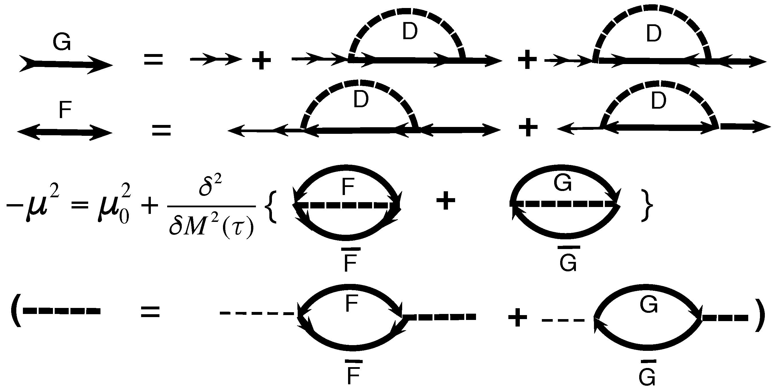
The Eliashberg equations, with instantonic propagator $\mathcal{D}\left(\tau \right)\cos ({\overrightarrow{Q}}_{AF}\cdot \overrightarrow{r})$ of (25) playing role of spin excitation mode for the Cooper pairing, differ from the common ones [1,4,15] by the self-consistency condition applied to the instantonic propagator $\mathcal{D}\left(\tau \right)$, as is explained in detail below and symbolically expressed in the last but one line in Figure 3. The last line in Figure 3 contains the ‘common’ third equation for the pairing boson propagator and is written in the brackets for comparison, see e.g., [1,4]. We derive the ‘Eliashberg equations’ using effective retarded interaction $D_i(\tau +{\tau }_0,{\tau }^{\prime }+{\tau }_0)$ in (13) substituted by the instantonic propagator $\mathcal{D}\left(\tau \right)\cos ({\overrightarrow{Q}}_{AF}\cdot \overrightarrow{r})$ from Equation (25). Then, the ‘usual’ integral equations for the self-energy functions ${\sum }_{1p,\sigma }$ and ${\sum }_{2p,\sigma }$ are obtained [15].The latter become much simplified under an assumption of the nesting with QSDW’s wave-vector $Q_{AF}$ and a d-wave symmetry of the superconducting order parameter in comparison with [15] (see Appendix A and Appendix B for details):

$${\displaystyle {\sum }_{1p,\sigma }\left(\omega \right)=\sum _{\Omega }\frac{{\mathcal{D}}_Q(\Omega )\left(-i(\omega -\Omega )-{\epsilon }_{p-Q}-{\sum }_{1p-Q,\sigma }^{*}(\omega -\Omega )\right)}{|-i(\omega -\Omega )+{\epsilon }_{p-Q}+{\sum }_{1,p-Q,\sigma }{(\omega -\Omega )|}^2+{|{\sum }_{2p-Q,\sigma }(\omega -\Omega )|}^2};}$$

(43)

$${\displaystyle {\sum }_{2p,\sigma }\left(\omega \right)=\sum _{\Omega }\frac{-{\mathcal{D}}_Q(\Omega ){\sum }_{2,p-Q,\sigma }(\omega -\Omega )}{|-i(\omega -\Omega )+{\epsilon }_{p-Q}+{\sum }_{1p-Q,\sigma }{(\omega -\Omega )|}^2+{|{\sum }_{2p-Q,\sigma }(\omega -\Omega )|}^2},}$$

(44)

where $\omega =\pi T(2m+1)$ and $\Omega =2\pi Tm$, $m=0,\pm 1,...$ are fermionic and bosonic frequencies, respectively [10], and here and everywhere below we use notation Q for the AF wave vector $Q_{AF}$ in order to simplify notations. The d-wave symmetry of Cooper pairing in combination with ‘nesting’ conditions for the bare fermionic dispersion leads to the following relations (compare [4]):

$${\epsilon }_{p-Q}=-{\epsilon }_p\equiv -\epsilon ;{\sum }_{2p-Q,\sigma }=-{\sum }_{2p,\sigma };{\sum }_{1p,\sigma }=-{\sum }_{1p-Q,\sigma }^{*};$$

(45)

$${\sum }_{1p,\sigma }\left(\omega \right)=f(\epsilon ,\omega )+is(\epsilon ,\omega );f(-\epsilon ,\omega )=-f(\epsilon ,\omega );s(\epsilon ,-\omega )=-s(\epsilon ,\omega ).$$

(46)

In the $k\to 1$ limit the saddle-point action (22) of the spin subsystem reaches the lowest value, while the instantons acquire a hyperbolic tangent form (23). Simultaneously, the instantonic propagator $\mathcal{D}\left(\tau \right)$ acquires the sawtooth shape (35). Under these conditions parameter q in (28) becomes small: $q\to 0$, and self-energy function ${\sum }_{1p,\sigma }$ (46) can be found in algebraic form (see Appendix A and Appendix B):

$${\sum }_{\sigma }(\epsilon ,\omega )=\epsilon \cdot f+i\omega \cdot s;$$

(47)

where f and s are slowly dependent on $\omega$ and $\epsilon$ functions.

Bound States Along the Axis of Matsubara Time

When conditions (47) hold, the second Eliashberg Equation (44) for superconducting self-energy ${\sum }_2(\epsilon ,\omega )$ is transformed into the Schrödinger’s equation on the Matsubara time axis of coordinates, with instantonic propagator $\mathcal{D}\left(\tau \right)$ playing a role of periodic ‘potential’. For this purpose we introduce definition of the ‘kernel’ $K\left(\tau \right)\equiv T{\sum }_{\omega }K\left(\omega \right)e^{-i\omega t}$:

$$K\left(\tau \right)=T\sum _{\omega }{\displaystyle \frac{e^{-i\omega t}}{{\omega }^2{(1-s)}^2+{\epsilon }^2{(1+f)}^2+{|{\sum }_2|}^2}}=\frac{\sinh \left[g\left(\frac{1}{2T}-\left|\tau \right|\right)\right]}{2g{(1-s)}^{2}cosh\left(\frac{g}{2T}\right)};$$

(48)

and:

$$g^2={\displaystyle \frac{{\epsilon }^2{(1+f)}^2+{|{\sum }_2|}^2}{{(1-s)}^2}}$$

(49)

The kernel possesses the following property:

$${\displaystyle \frac{{\partial }^{2}K\left(\tau \right)}{\partial {\tau }^2}}=g^{2}K\left(\tau \right)-\frac{\delta \left(\tau \right)}{{(1-s)}^2},$$

(50)

where $\delta \left(\tau \right)$ is Dirac Delta function. Above we have approximated self-energy in the denominator of the sum in (48) as $\omega$-independent function of energy $\epsilon$: ${\sum }_2(\epsilon ,\omega )\to {\sum }_2(\epsilon ,0)\equiv {\sum }_2$, provided, that $\omega$-dependence of the self-energy ${\sum }_2$ is slow enough and it can be taken at $\omega \approx 0$. Using definition (48) of the kernel $K\left(\tau \right)$ we introduce new unknown function $\sigma (\epsilon ,\tau )$ instead of ${\sum }_{2,\sigma }(\epsilon ,\omega )$ (the $\epsilon$ indices are dropped below to simplify notations):

$$\sigma \left(\omega \right)\equiv K\left(\omega \right){\sum }_2\left(\omega \right),\sigma \left(\tau \right)\equiv {\int }_0^{1/T}K\left(\tau -{\tau }^{\prime }\right){\sum }_2\left({\tau }^{\prime }\right)d{\tau }^{\prime },$$

(51)

$$\sigma \left(\tau +\frac{1}{T}\right)=-\sigma \left(\tau \right).$$

(52)

The last antisymmetry condition is due to Fermi-statistics. Then, we rewrite the second Eliashberg Equation (44) for superconducting self-energy ${\sum }_2(\epsilon ,\omega )$ in the integral form:

$$\sigma \left(\tau \right)={\int }_0^{1/T}K\left(\tau -{\tau }^{\prime }\right)\mathcal{D}\left({\tau }^{\prime }\right)\sigma \left({\tau }^{\prime }\right)d{\tau }^{\prime }.$$

(53)

Now, using property (50) of the kernel $K\left(\tau \right)$ and differentiating Equation (53) twice over $\tau$ we obtain the following Schrödinger like equation:

$$-{\sigma }^{″}\left(\tau \right)-\frac{1}{{(1-s)}^2}\mathcal{D}\left(\tau \right)\sigma \left(\tau \right)=-g^2\sigma \left(\tau \right);\mathcal{D}\left(\tau +\frac{1}{nT}\right)=\mathcal{D}\left(\tau \right),$$

(54)

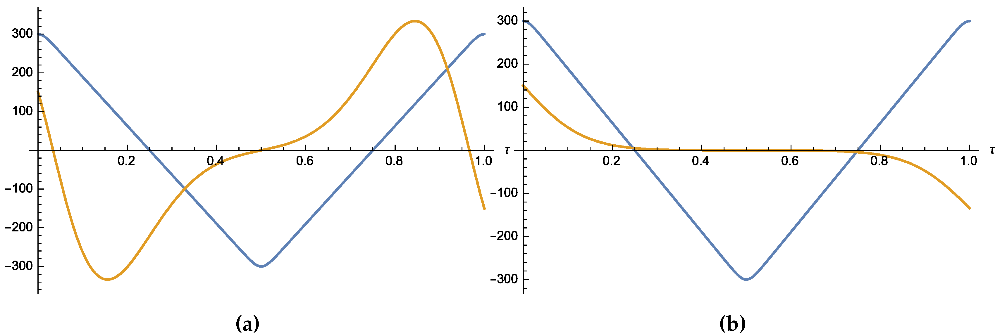
where, indeed, propagator $\mathcal{D}\left(\tau \right)$ plays the role of periodic ‘Bloch potential’, while unknown function $\sigma \left(\tau \right)$ plays the role of the ‘wave function’, with $-g^2$ being an eigenvalue. In Figure 4 the instantonic propagator (32) is plotted (blue line), thus manifesting a ‘sawtooth’ curve. According to (52) the ‘wave function’ should posses at least one (odd number of) zero inside the interval $\{0,1/T\}$ of Matsubara slab. Hence, we are looking for the first excited state with eigenvalue $E_1=-g_1^2$, which is closest one to the bottom of the ‘energy band’. The ground state wave function does not posses zeroes, according to quantum mechanics, and is real and periodic by virtue of the Bloch’s theorem, see e.g., [14]. Examples of a single zero and a triple zero wave functions, that were calculated numerically, are plotted in Figure 4. Now, substituting (35) into (54) we find the following equivalent equation within a single period $1/nT$ of the ‘potential’ $\mathcal{D}\left(\tau \right)$:

$$-{\sigma }^{″}\left(\tau \right)+\frac{{\mu }^{2}4nT}{2\lambda {(1-s)}^2}|\tau |\sigma \left(\tau \right)=\left(\frac{{\mu }^2}{2\lambda {(1-s)}^2}-g^2\right)\sigma \left(\tau \right),-\frac{1}{2nT}\le \tau \le \frac{1}{2nT}.$$

(55)

According to Figure 4b, the lowest possible eigenvalue, $-g_1^2$, could be approximated by the minimal value of the sawtooth potential itself, thus, leading to the following solution of the second Eliashberg Equation (44):

$${\epsilon }^2{(1+f)}^2+{|{\sum }_2|}^2=g_1^2{(1-s)}^2\approx \frac{{\mu }^2}{2\lambda }.$$

(56)

Hence, nonzero self-energy ${\sum }_2$ exists in the interval of energies around the Fermi-level, $\{-{\epsilon }_M,{\epsilon }_M\}$:

$$-{\epsilon }_M\le \epsilon \le {\epsilon }_M;{\epsilon }_M^2\equiv \{g_1^2\frac{{(1-s)}^2}{{(1+f)}^2},w^2\}{|}_{min},$$

(57)

where w is a width of the energy interval around the bare chemical potential, inside which the nesting condition (45) holds. Other solutions with smaller eigenvalues $-g^2$ do exist as well, see e.g., Figure 4a, $g_3^2=0;{\sum }_2\equiv 0$, but they correspond to excited states of Cooper-pairs condensate.

4. Instanton Driven ‘Strange Metal’ and Superconducting Transitions

Now we use standard procedure [10] to calculate free energy change $\Delta \Omega$ per ‘spin-bag’ due to instanton-mediated superconducting pairing (thus dropping the spin-bag index i introduced in (4)):

$$\Delta {\Omega }_s=-T\ln {\displaystyle \frac{Tr\left\{e^{-{\int }_0^{\beta }{H}_{int}\left(\tau \right)d\tau }\mathcal{G}\left(0\right)\right\}}{Tr\left\{\mathcal{G}\left(0\right)\right\}}}\equiv {\Omega }_s-{\Omega }_0;\mathcal{G}\left(0\right)\equiv e^{-\beta H_0};$$

(58)

$$H_{int}=\left(c_{q+Q,s}^{+}{M}_0\left(\tau \right)s{c}_{q,s}+H.c.\right)$$

(59)

where $H_0$ is the first term in the sum in (4) respectively. We use the instantonic amplitude $\alpha$ defined in (33), as a formal variable coupling strength in the spin-fermion interaction Hamiltonian $H_{int}$ in (59) and calculate the free energy derivative:

$${\displaystyle \frac{\partial {\Omega }_s}{\partial \alpha }}=T{\int }_0^{\beta }〈{\displaystyle \frac{\partial H_{int}\left(\tau \right)}{\partial \alpha }}〉d\tau =-\frac{T}{\alpha }{{\int }_0^{\beta }\int }_0^{\beta }〈\langle H_{int}\left(\tau \right)H_{int}\left({\tau }^{\prime }\right)〉{\rangle }_{{\tau }_0}d\tau d{\tau }^{\prime },$$

(60)

where thermodynamic averaging in (60) together with an averaging over the ‘zero mode’ shift ${\tau }_0$ of the instantons leads to the following relation, see Appendix A and Appendix B:

$$\begin{array}{c}{\displaystyle \frac{\partial {\Omega }_s}{\partial \alpha }}=\frac{T^2}{\alpha }\sum _{\Omega ,\omega p,\sigma }\mathcal{D}(\Omega )\left\{{\displaystyle \frac{{\overline{\sum }}_{2,p-Q,\sigma }\left(\omega \right){\sum }_{2p,\sigma }(\omega -\Omega )+{\sum }_{2,p-Q,\sigma }\left(\omega \right){\overline{\sum }}_{2p,\sigma }(\omega -\Omega )}{\mathsf{\Phi }\left(\omega \right)\mathsf{\Phi }(\omega -\Omega )}}+\right.\hfill \\ \left.+{\displaystyle \frac{2Re\left[(i\omega +{\epsilon }_p-{\sum }_{1,p,\sigma }\left(\omega \right))(i(\omega -\Omega )+{\epsilon }_{p-Q}-{\sum }_{1,p-Q,\sigma }(\omega -\Omega ))\right]}{\mathsf{\Phi }\left(\omega \right)\mathsf{\Phi }(\omega -\Omega )}}\right\}\hfill \end{array}$$

(61)

where:

$$\mathsf{\Phi }\left(\omega \right)=(i\omega -{\epsilon }_p-{\sum }_{1,p,\sigma }\left(\omega \right))(i\omega +{\epsilon }_p+{\sum }_{1,p,\sigma }^{*}\left(\omega \right))-{\sum }_{2p,\sigma }\left(\omega \right){\overline{\sum }}_{2p,\sigma }\left(\omega \right)$$

(62)

Now, we take into account ‘nesting’ conditions with vector ${\overrightarrow{Q}}_{AF}$ expressed in (45) and (46), and further use definition of ‘kernel’ $K\left(\omega \right)$ in (48) in combination with Eliashberg Equations (43) and (44). Along this route we finally obtain, after subtraction of the ‘normal state’ free energy, $\Delta {\Omega }_s\equiv {\Omega }_1-{\Omega }_1({\sum }_2=0)$, the following expression:

$${\displaystyle \frac{\partial \Delta {\Omega }_s}{\partial \alpha }}=-\frac{2T}{\alpha }\sum _{\omega ,p,\sigma }K\left(\omega \right){\left|{{\displaystyle \sum }}_{2,p,\sigma }\left(\omega \right)\right|}^2\approx -\frac{\tanh \left(g_1/2T\right)}{\alpha {(1-s)}^2{g}_1}\sum _{p,\sigma }{\left|{{\displaystyle \sum }}_{2,p,\sigma }(\omega =0)\right|}^2,$$

(63)

where we had inferred $K(\tau =0)$ from (48) and approximated self-energy ${\sum }_{2,p,\sigma }\left(\omega \right)$ with a frequency independent function of momentum p at $\omega =0$. Now, we use solution (56) for the self-energy ${\sum }_2$ and pass from summation over momentum p to an integration over energy $\epsilon =\epsilon \left(p\right)$, simultaneously introducing a bare density of states ${\nu }_0$ in the vicinity of the Fermi-level. Then, relation (63) further yields:

$$\begin{array}{c}\frac{\partial \Delta {\Omega }_s}{\partial \alpha }=-\frac{2{\nu }_0}{\alpha g_1}\tanh \left({\displaystyle \frac{g_1}{2T}}\right)\underset{0}{\overset{{\epsilon }_M}{\int }}d\epsilon \left[{g_1}^2-{\epsilon }^2{\displaystyle \frac{{(1+f)}^2}{{(1-s)}^2}}\right]=\hfill \\ =-\frac{2{\nu }_0}{\alpha g_1}\tanh \left({\displaystyle \frac{g_1}{2T}}\right)\left[{g_1}^2{\epsilon }_M-\frac{{\epsilon }_M^3}{3}{\displaystyle \frac{{(1+f)}^2}{{(1-s)}^2}}\right]\hfill \end{array}$$

(64)

where upper limit of integration ${\epsilon }_M$ is defined in (57). To proceed, one uses the following relation that follows from Equations (17), (28) and (33):

$$g_1^2\equiv {\alpha }^2{A}^2\approx \frac{{\mu }^2}{2\lambda {(1-s)}^2};A^2=\frac{{\pi }^2}{8q^2{(1-s)}^2}.$$

(65)

Following the well known procedure of calculation of the free energy of an interacting system [10], we substitute $\alpha \to x$ in (64) and integrate over x from 0 to $\alpha$, thus, finding $\Delta {\Omega }_s$:

$$\Delta {\Omega }_s={\int }_0^{\alpha }{\displaystyle \frac{\partial \Delta \Omega }{\partial x}}dx=-\frac{4{\nu }_0}{3}\left|\frac{1-s}{1+f}\right|A^2{\int }_0^{\alpha }x\tanh \left({\displaystyle \frac{xA}{2T}}\right)dx.$$

(66)

Before we proceed one important observation is in order. The above integration in (66) neglects dependence of coefficients $f,s$ on $\alpha$: see Equations (81)–(85). This leads to a simplified result for $T^{*}$ below, (86). When allowing for $\alpha$ dependence of $f,s$ one finds more involved expression for $T^{*}$, (87), that results in Figure 5. A detailed derivation will be published in the paper under preparation. Now, neglecting mentioned above effect, we obtain a simple expression, that depending on ratio $\alpha A/2T$, has two limits:

$$\Delta {\Omega }_s=-\frac{2\widetilde{{\nu }_0}}{3}\left\{\begin{array}{c}{\displaystyle \frac{{\alpha }^3{A}^3}{3T}}\equiv {\displaystyle \frac{{\left(g_1^2\right)}^{3/2}}{3T}};\alpha A/2T\ll 1;\hfill \\ {\alpha }^2{A}^2\equiv g_1^2;\alpha A/2T\gg 1.\hfill \end{array}\right.;\widetilde{{\nu }_0}\equiv {\nu }_0\left|\frac{1-s}{1+f}\right|.$$

(67)

Now, using (67), one is in a position to find self-consistently a phase transition from the bare ‘spin-wave’ Lagrangian to an ‘instantonic’ Lagrangian, as is indicated in (14), which is induced by Cooper pairing fluctuations. Namely, in the above derivation of (67) an instantonic pairing ‘glue’ propagator (32) was used to evaluate the lowest energy eigenvalue $-g_1^2$ of the ‘Schrödinger’s’ Equation (54). Hence, using (67), we can relate a value of the free energy per ‘spin-bag’ decrease due to superconducting fluctuations, $\Delta {\Omega }_s$, to pairing ‘glue’ amplitude, $g_1^2{(1-s)}^2\approx {\mu }^2/2\lambda$, and infer from this a mechanism of (sign) change of the pre-factor: ${\mu }_0^2\to -{\mu }^2$ in the Lagrangian (14). A value of parameter $\mu$ has to be determined self-consistently, which is described in the next subsection.

4.1. Self-Consistency Equation for Instantonic Phase Formation

An idea of the following derivation is to cast energy decrease (67) into a form:

$$\Delta {\Omega }_s=-2c^{2}T\underset{0}{\overset{\beta }{\int }}d\tau \frac{1}{2g_{sf}{U}^2}{M}_0^2\left(\tau \right),$$

(68)

which then leads to the following expression for effective Euclidean action ${\tilde{S}}_0$ of the system:

$${\tilde{S}}_0={\displaystyle \frac{\Delta {\Omega }_s}{T}}+\underset{0}{\overset{\beta }{\int }}d\tau L_{AF}^0=\underset{0}{\overset{\beta }{\int }}d\tau \frac{1}{2g_{sf}{U}^2}\left\{{\dot{M}}^2-2\frac{{\mu }^2}{\lambda }{M}^2+M^4\right\};$$

(69)

$$\begin{array}{c}{\mu }^2+{\mu }_0^2=c^2.\hfill \end{array}$$

(70)

Here (70) follows immediately from definitions (68), (69), and (14). In order to find coefficient $c^2$ from (68), we calculate variation of the both sides of equality (68) under an infinitesimal variation of the function $M_0\left(\tau \right)$ at a time instant $\tau$. The variation of the left hand side of (68), $\Delta {\Omega }_s$, can be found using well known formula [16], that relates variation of e.g., eigenvalue $-g_1^2$ of the Schrödinger’s Equation (54) to an infinitesimal change of potential $\mathcal{D}\left(\tau \right)$ at a time instant $\tau$:

$$\delta {g_1^2}_{\tau }=\frac{1}{{(1-s)}^2}\delta \mathcal{D}\left(\tau \right){\sigma }_1^{*}\left(\tau \right){\sigma }_1\left(\tau \right),$$

(71)

where ${\sigma }_1\left(\tau \right)$ is eigenfunction of the Schrödinger’s Equation (54) corresponding to the eigenvalue $-g_1^2$, and variation of the potential is derived readily from (25):

$$\delta \mathcal{D}\left(\tau \right)=\delta M\left(\tau \right)M_0\left(2\tau \right).$$

(72)

Substituting (72) into (71) we obtain:

$$\delta {g_1^2}_{\tau }=\frac{1}{{(1-s)}^2}\delta M\left(\tau \right)M_0\left(2\tau \right){\sigma }_1^{*}\left(\tau \right){\sigma }_1\left(\tau \right)$$

(73)

Choosing a zero origin of the Matsubara time interval $\{0,1/T\}$ at $M_0\left(\tau =0\right)=0$ and taking into account strong localisation of the eigenfunction ${\sigma }_1\left(\tau \right)$ in the vicinities of the minima of potential $\mathcal{D}\left(\tau \right)$, see Figure 4b, we rewrite (73):

$$\delta {g_1^2}_{\tau }=\frac{2}{{(1-s)}^{2}n}\delta M\left(\tau \right)M_0\left(\tau \right),$$

(74)

where factor $1/n$ arises due to normalisation of the eigenfunction ${\sigma }_1\left(\tau \right)$ in the n minima of potential $\mathcal{D}\left(\tau \right)$ possessing period $1/nT$. Using (74), it is straightforward to find variation of $\Delta {\Omega }_s$:

$$\delta {\left\{\Delta {\Omega }_s\right\}}_{\tau }=-\frac{2\widetilde{{\nu }_0}}{3}\delta M\left(\tau \right)M_0\left(\tau \right)\left\{\begin{array}{c}{\displaystyle \frac{g_1}{T{(1-s)}^{2}n}};g_1/2T\ll 1;\hfill \\ {\displaystyle \frac{2}{{(1-s)}^{2}n}};g_1/2T\gg 1.\hfill \end{array}\right..$$

(75)

Simultaneously, variation of the right hand side of (68) is found trivially:

$$\delta {\left\{-2c^{2}T\underset{0}{\overset{\beta }{\int }}d\tau \frac{1}{2g_{sf}{U}^2}{M}_0^2\left(\tau \right)\right\}}_{\tau }=-\frac{2c^2}{g_{sf}{U}^2}\delta M\left(\tau \right)M_0\left(\tau \right).$$

(76)

Now, equating results in (75) and (76) and using Equation (80) and known value of $g_1$ from (56) one finds self-consistency equation for the pre-factor ${\mu }^2$ of the effective instantonic action (69):

$$c^2\equiv {\mu }^2+{\mu }_0^2=\frac{\widetilde{{\nu }_0}{g}_{sf}{U}^2}{3}\left\{\begin{array}{c}{\displaystyle \frac{\mu }{T\sqrt{2\lambda }{|1-s|}^{3}n}};{\displaystyle \frac{\mu }{2T\sqrt{2\lambda }|1-s|}}\ll 1;\hfill \\ {\displaystyle \frac{2}{{(1-s)}^{2}n}};{\displaystyle \frac{\mu }{2T\sqrt{2\lambda }|1-s|}}\gg 1.\hfill \end{array}\right.$$

(77)

Hence, we found that positive bare coefficient ${\mu }_0^2$ in the Lagrangian may turn into a negative coefficient $-{\mu }^2$ in the effective Lagrangian (14) due to Cooper pair condensate formation, thus manifesting formation of an ‘instantonic phase’. The latter would be manifested by a nonzero constant $g_1^2$, see (56) and Figure 4.

4.2. ‘Strange Metal’ Phase Below Transition Temperature T*

Our strategy is to investigate evolution with temperature of the Euclidean action $S_0\left(T\right)$ of the system (24), starting from origination of the instantonic phase, $S_0\left(T^{*}\right)>0$ (likely called ‘strange metal’ phase in high-$T_c$ cuprates), until transition to superconducting phase, $S_0\left(T_c\right)<0$. We proceed by solving Equations (77) simultaneously with Eliashberg equations for the constants f and s, defined in (47), that follow from (43), see Appendix A and Appendix B. First, consider the ‘high temperatures’ interval $g_1/2T\ll 1$. Then, the first of the Equations (77) constitutes a quadratic equation, and together with equations for the constants f and s read:

$$\begin{array}{c}{\mu }^2-{\displaystyle \frac{2{\tilde{G}}^2}{T}}\mu +{\mu }_0^2=0;{\tilde{G}}^2={\displaystyle \frac{\widetilde{{\nu }_0}{g}_{sf}{U}^2}{6\sqrt{2\lambda }{|1-s|}^{3}n}};\widetilde{{\nu }_0}\equiv {\nu }_0\left|{\displaystyle \frac{1-s}{1+f}}\right|\hfill \end{array}$$

(78)

$$\begin{array}{c}{s}^2-s+G^2=0;G^2\equiv {\displaystyle \frac{{\mu }^2}{24\lambda n^2{T}^2}};{\left({\displaystyle \frac{g_1}{2T}}\right)}^2={\displaystyle \frac{{\mu }^2}{8\lambda T^2{(1-s)}^2}}\ll 1\hfill \end{array}$$

(79)

$$\begin{array}{c}f+1={\displaystyle \frac{G^2}{G^2-s^2}}.\hfill \end{array}$$

(80)

An inequality in (79) hints to smallness of $G^2$ parameter, leading indeed, to a consistent solution:

$$\begin{array}{c}{s}_{\pm }=\frac{1}{2}\left(1\pm \sqrt{1-4G^2}\right);\hfill \end{array}$$

(81)

$$\begin{array}{c}{s}_{-}\approx G^2;f_{-}={\displaystyle \frac{s_{-}^2}{G^2-s_{-}^2}}\approx G^2;\hfill \end{array}$$

(82)

$$\begin{array}{c}\widetilde{{\nu }_0}\equiv {\nu }_0\left|{\displaystyle \frac{1-s}{1+f}}\right|\approx {\nu }_0;\hfill \end{array}$$

(83)

$$\begin{array}{c}{\mu }_{\pm }={\displaystyle \frac{{\tilde{G}}^2}{T}}\pm \sqrt{{\displaystyle \frac{{\tilde{G}}^4}{T^2}}-{\mu }_0^2};\hfill \end{array}$$

(84)

$$\begin{array}{c}{\tilde{G}}^2\approx {\displaystyle \frac{{\nu }_0{g}_{sf}{U}^2}{6\sqrt{2\lambda }n}}.\hfill \end{array}$$

(85)

The choice of “−” sign in (81) is dictated by consistency with inequality (79). Hence, from (84) one readily finds a temperature $T^{*}$, at which transition to an instantonic phase first takes place:

$$T^{*}={\displaystyle \frac{{\tilde{G}}^2}{{\mu }_0}}|n=1\approx {\displaystyle \frac{{\nu }_0{g}_{sf}{U}^2}{6\sqrt{2\lambda }{\mu }_0}}$$

(86)

In relation with remark made after Equation (66), an account of $s,f$ dependence on $\alpha$ leads to a more involved relation (derivation is pending in the paper under preparation):

$${T^{*}}^2={\displaystyle \frac{{\left({\nu }_0{g}_{sf}{U}^2\right)}^2}{36{\left({\mu }_0\sqrt{\lambda }\right)}^2}}\left[1\pm \sqrt{1-{\displaystyle \frac{12{\mu }_0^4}{{\left({\nu }_0{g}_{sf}{U}^2\right)}^2}}}\right],$$

(87)

where the upper sign brunch leads to result (86), while the lower sign brunch leads to a saturation of $T^{*}$ at ${\mu }_0/\left(\sqrt{6\lambda }\right)$ in the large limit of dimensionless coupling constant $g=\sqrt{{\nu }_0{g}_{sf}{U}^2}/{\mu }_0$. The two branches of the instantonic amplitude ${\mu }_{\pm }$ originate at $T^{*}$ according to (84), and split in the temperatures interval $T^{*}>T>T_c$ while starting from the common initial value ${\mu }_{\pm }(T=T^{*})={\mu }_0$:

$$\begin{array}{c}{\mu }_{+}\left(T\right)\approx 2{\displaystyle \frac{{\tilde{G}}^2}{T}};\hfill \end{array}$$

(88)

$$\begin{array}{c}{\mu }_{-}\left(T\right)\approx T{\displaystyle \frac{{\mu }_0^2}{2{\tilde{G}}^2}};T^{*}>>T>T_c\hfill \end{array}$$

(89)

where both expressions are given in the ‘low temperature’ limit $T_c<<T<<T^{*}$. In order for these solutions to exist the following condition must hold:

$$G\left(T^{*}\right)={\displaystyle \frac{\mu \left(T^{*}\right)}{2\sqrt{6\lambda }{T}^{*}}}\equiv {\displaystyle \frac{{\mu }_0^2}{\sqrt{3}{\nu }_0{g}_{sf}{U}^2}}<1/2.$$

(90)

Thus, temperature dependences of the Euclidean action $S_0\left(T\right)$ of the system (24) corresponding to the two instantonic brunches ${\mu }_{\pm }\left(T\right)$ differ. While branch ${\mu }_{+}\left(T\right)$ finally leads to a condensation of Cooper pairs in superconducting state at $T_c$, the other branch ${\mu }_{-}\left(T\right)$ remains a (macroscopic) fluctuation mode, that gradually softens ($S_0\left({\mu }_{-}\left(T\right)\right)\propto T^3$) as the temperature decreases.

4.3. Superconducting Transition Inside the Instantonic Phase: T_c

Consider now an expression for the effective Euclidean action $S_0\left(T\right)$ of the system (24) with normal metal Euclidean action being subtracted, see (69). It is obvious, that transition from instantonic phase to superconducting thermal equilibrium state is manifested by $S_0\left(T\right)$ becoming negative. Hence, equation that defines superconducting transition temperature $T_c$ is just:

$${\tilde{S}}_0\left(T_c\right)=\frac{1}{2g_{sf}{U}^2}\left\{2n\left(\frac{2\sqrt{2}\mu {\left(T_c\right)}^3}{3\lambda }\right)-\frac{\mu {\left(T_c\right)}^4}{T_c\lambda }\right\}=0;n=1.$$

(91)

It is straightforward to infer from (91) and definition (65) that:

$$\frac{\mu \left(T_c\right)}{T_c\sqrt{\lambda }}=2\left(\frac{2\sqrt{2}}{3\sqrt{\lambda }}\right);{\displaystyle \frac{g_1}{2T_c}}={\displaystyle \frac{\mu \left(T_c\right)}{2T_c\sqrt{2\lambda }|1-s|}}\equiv {\displaystyle \frac{2}{3\sqrt{\lambda }|1-s|}}\gg 1.$$

(92)

Hence, in the vicinity of $T_c$ one has to use the second of Equations (77) and also equations for the constants f and s, that are valid in the limit: ${\displaystyle \frac{g_1}{2T_c}}\gg 1$ (see Appendix A and Appendix B):

$$\begin{array}{c}{\mu }^2+{\mu }_0^2=\frac{2\widetilde{{\nu }_0}{g}_{sf}{U}^2}{3{(1-s)}^2};\hfill \end{array}$$

(93)

$$\begin{array}{c}{s}^2-s-G_1^2=0;G_1^2\equiv {\displaystyle \frac{2{\mu }^2}{\lambda g_1^2}};\hfill \end{array}$$

(94)

$$\begin{array}{c}f={\displaystyle \frac{s^2}{G_1^2-s^2}}.\hfill \end{array}$$

(95)

$$\begin{array}{c}{g}_1^2={\displaystyle \frac{{\mu }^2}{2\lambda {(1-s)}^2}}.\hfill \end{array}$$

(96)

Next, one substitutes (94) into (95), and also (96) into (94), leading after a simple algebra to the following relations:

$$\begin{array}{c}\hfill f=-s;\left\{\begin{array}{c}s=1;\hfill \\ s=\frac{4}{3}.\hfill \end{array}\right.\end{array}$$

(97)

Then, a choice consistent with inequality (96) and finiteness of the instantonic amplitude in (93) would be:

$$s=-f=\frac{4}{3}.$$

(98)

Finally, substituting (98) into (93) one finds $T_c$ from (92):

$$T_c=\frac{3}{4\sqrt{2}}{\left(6{\nu }_0{g}_{sf}{U}^2-{\mu }_0^2\right)}^{1/2}.$$

(99)

It is interesting to observe, that a necessary condition for existence of solution for $T_c$ follows from (99):

$${\displaystyle \frac{{\nu }_0{g}_{sf}{U}^2}{{\mu }_0^2}}>{\displaystyle \frac{1}{6}},$$

(100)

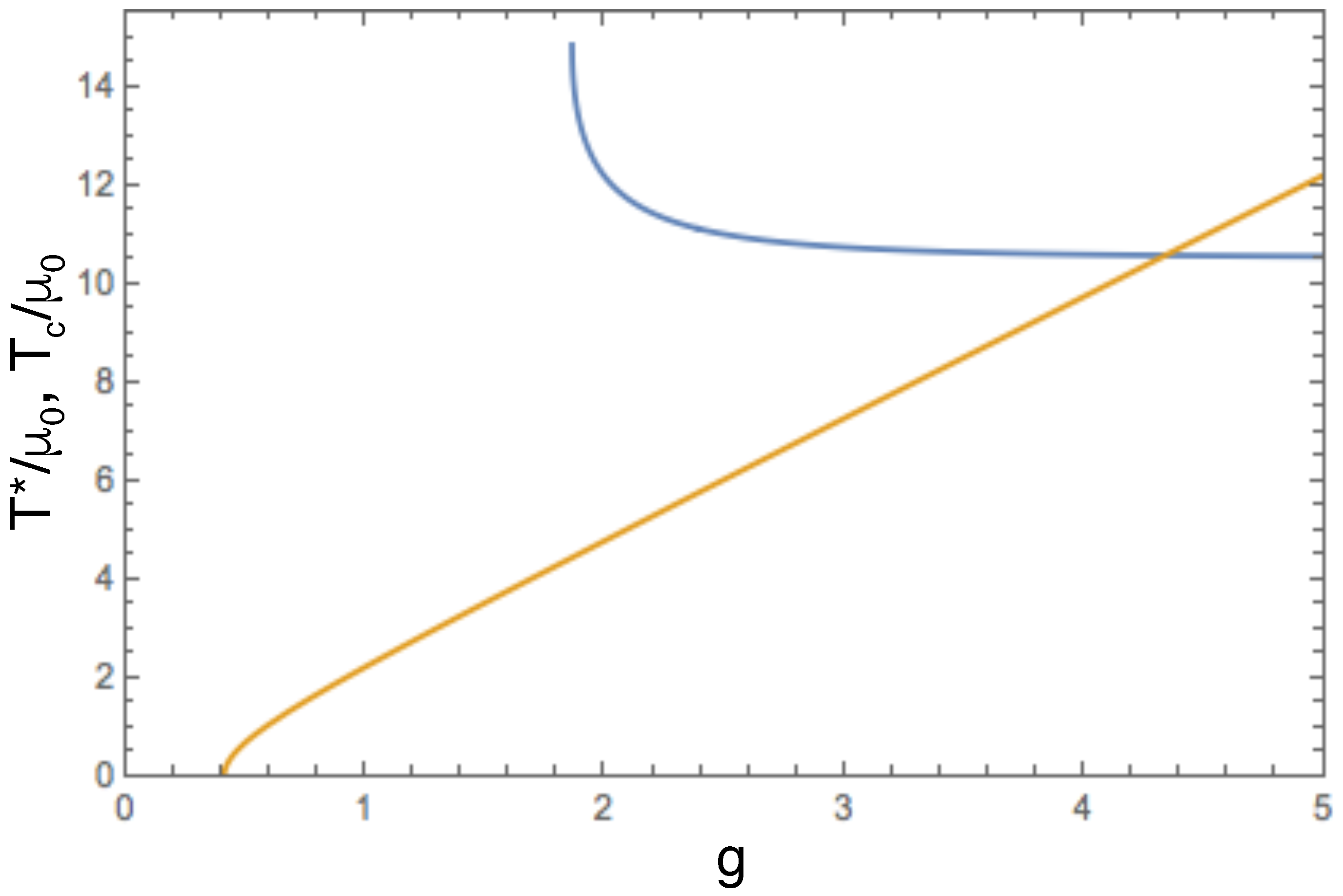
and is less restrictive than condition for existence of $T^{*}$ solution in (87): ${\nu }_0{g}_{sf}{U}^2/{\mu }_0^2>\sqrt{12}$. Thus, there may exist an interval of intermediate coupling strength, $1/6<{\nu }_0{g}_{sf}{U}^2/{\mu }_0^2<\sqrt{12}$, in which $T_c$ is not preceded by $T^{*}$, i.e., ‘strange metal’ phase is absent above the superconducting dome. This feature is indeed present in the phase diagram of high-$T_c$ cuprates in the ‘underdoped’ regime [17,18,19]. Both transition temperatures are found from Eliashberg like system of equations, but with spin wave instantonic propagator playing role of pairing boson. Figure 5 contains plots of the analytically evaluated $T^{*}$, (86), and $T_c$, (99), dependences on effective instanton-fermion dimensionless coupling strength $g=\left(\sqrt{{\nu }_0{g}_{sf}}U\right)/{\mu }_0$, that surprisingly resemble phase diagram in the temperature-doping coordinates, see e.g., [17,18,19]. To get the second part of the superconducting $T_c$ dome in the ‘overdoped’ region of high-$T_c$ cuprates an assumption should be made on the dependences on doping of e.g., bare density of ‘nested’ fermionic states ${\nu }_0$, (64), and related cut-off energy ${\epsilon }_M$, (57). Simultaneously, a numerical self-consistent solution of the ‘Eliashberg equations’ (43), (44), and (76) in the whole interval of coupling g should be made. Finally, we mention that transition temperatures $T^{*}$ and $T_c$ derived above depend on the powers of $\sqrt{{\nu }_0{g}_{sf}}U$, rather than on $U\exp \{-1/\left({\nu }_0{g}_{sf}\right)\}$ typical for a weak-coupling BCS theory, compare e.g., [2].

5. Conclusions

To summarise, an instantonic mechanism of high temperature superconductivity is proposed as part of a wider picture. Namely, it is demonstrated that in principle, an instantonic quantum nematic can emerge as a ‘hidden order’, that self-consistently provides pairing glue for Cooper pairs. This may happen as a 1-st order phase transition, since according to Equation (84), the negative sign coefficient $-2{{\mu }_0}^2/\lambda$ appears discontinuously at transition temperature $T^{*}$, when it substitutes the bare positive coefficient $2{{\mu }_0}^2/\lambda$ in front of the quadratic term in the effective AF spin action (5). Since the instantonic action of a QSDW-populated ‘spin-bag’ (24), (69) remains positive in the interval of temperatures $T_c<T<T^{*}$, the ‘spin-bags’ could be considered as fluctuations of ‘annealed’ type with preformed Cooper pairs inside. At superconducting $T_c$ the instantonic action of ‘spin-bag’ passes zero and becomes negative at $T<T_c$ according to (91). Hence, the ‘spin-bags’ condense, becoming a ‘quenched’ quantum disorder, that is dressed with the condensate of Cooper pairs. The picture may be different, since depending on the strength of effective spin-fermion coupling, a temperature of nematic phase transition, $T^{*}$, either precedes superconducting transition temperature $T_c$, or ceases to exist, with instantonic quantum nematic condensing together with the superconducting Cooper pairs. Quantumness of emergent nematic state is provided by periodic in Matsubara time instantonic modulation of the amplitude of ‘hidden’ QSDW order. A detailed calculation of the measurable characteristics of the instanton-anti-instanton populated ‘spin-bags’ phases in 2+1D spin-fermion system is in progress and will be presented elsewhere.

References

- Abanov, A.; Chubukov, A.V.; Schmalian, J. Quantum-critical theory of the spin-fermion model and its application to cuprates: Normal state analysis. Adv. Phys. 2003, 52, 119–218. [Google Scholar] [CrossRef] [Green Version]
- Chubukov, A.V.; Schmalian, J. Superconductivity due to massless boson exchange in the strong-coupling limit. Phys. Rev. B 2005, 72, 174520. [Google Scholar] [CrossRef]
- Vojta, M.; Buragohain, C.; Sachdev, S. Quantum impurity dynamics in two-dimensional antiferromagnets and superconductors. Phys. Rev. B 2000, 61, 15152. [Google Scholar] [CrossRef]
- Efetov, K.B.; Meier, H.; Pépin, C. Pseudogap state near a quantum critical point. Nat. Phys. 2013, 9, 442–446. [Google Scholar] [CrossRef]
- Deng, H.Y. Spin glass behaviors compatible with a Zhang–Rice singlet within an effective model for cuprate superconductors. J. Phys. Condens. Matter 2009, 21, 075702. [Google Scholar] [CrossRef] [PubMed]
- Hussein, M.S.D.A.; Daghofer, M.; Dagotto, E.; Moreo, A. Phenomenological three-orbital spin-fermion model for cuprates. Phys. Rev. B 2018, 98, 035124. [Google Scholar] [CrossRef]
- Scheurera, M.S.; Chatterjeea, S.; Wub, W.; Ferrero, M.; Georges, A.; Sachdev, S. Topological order in the pseudogap metal. Proc. Natl. Acad. Sci. USA 2018, 115, E3665–E3672. [Google Scholar] [CrossRef] [Green Version]
- Chatterjee, S.; Sachdev, S.; Scheurer, M.S. Intertwining Topological Order and Broken Symmetry in a Theory of Fluctuating Spin-Density Waves. Phys. Rev. Lett. 2017, 119, 227002. [Google Scholar] [CrossRef] [Green Version]
- Mukhin, S.I. Spontaneously broken Matsubara’s time invariance in fermionic system: Macroscopic quantum ordered state of matter. J. Supercond. Nov. Magn. 2011, 24, 1165–1171. [Google Scholar] [CrossRef]
- Abrikosov, A.A.; Gor’kov, L.P.; Dzyaloshinski, I.E. Methods of Quantum Field Theory in Statistical Physics; Dover Publications: New York, NY, USA, 1963. [Google Scholar]
- Polyakov, A.M. Guage Fields and Strings; Harwood Academic Publishers: Amsterdam, The Netherlands, 1987. [Google Scholar]
- Mukhin, S.I. Euclidean action of fermi-system with hidden order. Phys. B Phys. Conden. Matter 2015, 460, 264–267. [Google Scholar] [CrossRef]
- Mukhin, S.I. Euclidian Crystals in Many-Body Systems: Breakdown of Goldstone’s Theorem. J. Supercond. Nov. Magn. 2014, 27, 945–950. [Google Scholar] [CrossRef]
- Witteker, E.T.; Watson, G.N. A Course of Modern Analysis; Cambridge University Press: Cambridge, UK, 1996. [Google Scholar]
- Eliashberg, G.M. Interactions between electrons and lattice vibrations in a superconductor. JETP 1960, 11, 696–702. [Google Scholar]
- Dashen, R.G.; Hasslacher, B.; Neveu, A. Semiclassiacl bound states in an asymptotically free theory. Phys. Rev. D 1975, 12, 2443–2458. [Google Scholar] [CrossRef]
- Zhang, H.; Sato, H. Universal relationship between Tc and the hole content in p-type cuprate superconductors. Phys. Rev. Lett. 1993, 70, 1697. [Google Scholar] [CrossRef]
- Tallon, J.L.; Bernhard, C.; Shaked, H.; Hitterman, R.L.; Jorgensen, J.D. Generic superconducting phase behavior in high-Tc cuprates: Tc variation with hole concentration in YBa2Cu307-δ. Phys. Rev. B 1995, 51, 12911–12914. [Google Scholar] [CrossRef]
- Chen, H.-D.; Capponi, S.; Alet, F.; Zhang, S.-C. Global phase diagram of the high-Tc cuprates. Phys. Rev. B 2004, 70, 024516. [Google Scholar] [CrossRef]
Figure 1.
Instanton-mediated Cooper-pairing below .
Figure 2.
Schematic plot of a periodic saddle-point solution (20) with the number of instanton-anti-instanton pairs . An arbitrary shift along the Matsubara axis is indicated with the dashed line, its significance is discussed in the text.
Figure 3.
The Eliashberg equations, with instantonic spin excitation propagator of (25) displaying Cooper pairing boson.
Figure 4.
Effective ‘Bloch potential’ (blue line) and eigen ‘wave function’ (yellow line) corresponding to the following set of parameters: , , ; (a) ; (b) .
Figure 5.
Analyticallyevaluated schematic plot of the instanton mediated Cooper-pairing (blue line) and superconducting (yellow line) dependences on effective instanton-fermion dimensionless coupling strength .
© 2018 by the author. Licensee MDPI, Basel, Switzerland. This article is an open access article distributed under the terms and conditions of the Creative Commons Attribution (CC BY) license (http://creativecommons.org/licenses/by/4.0/).
Share and Cite
MDPI and ACS Style
Mukhin, S. Negative Energy Antiferromagnetic Instantons Forming Cooper-Pairing ‘Glue’ and ‘Hidden Order’ in High-Tc Cuprates. Condens. Matter 2018, 3, 39. https://doi.org/10.3390/condmat3040039
AMA Style
Mukhin S. Negative Energy Antiferromagnetic Instantons Forming Cooper-Pairing ‘Glue’ and ‘Hidden Order’ in High-Tc Cuprates. Condensed Matter. 2018; 3(4):39. https://doi.org/10.3390/condmat3040039
Chicago/Turabian StyleMukhin, Sergei. 2018. "Negative Energy Antiferromagnetic Instantons Forming Cooper-Pairing ‘Glue’ and ‘Hidden Order’ in High-Tc Cuprates" Condensed Matter 3, no. 4: 39. https://doi.org/10.3390/condmat3040039