Dispersion and Damping of Phononic Excitations in Fermi Superfluid Gases in 2D

Abstract

We calculate the sound velocity and the damping rate of the collective excitations of a 2D fermionic superfluid in a non-perturbative manner. Specifically, we focus on the Anderson–Bogoliubov excitations in the BEC-BCS crossover regime, as these modes have a sound-like dispersion at low momenta. The calculation is performed within the path-integral formalism and the Gaussian pair fluctuation approximation. From the action functional, we obtain the propagator of the collective excitations and determine their dispersion relation by locating the poles of this propagator. We find that there is only one kind of collective excitation, which is stable at $T=0$ and has a sound velocity of $v_F/\sqrt{2}$ for all binding energies, i.e., throughout the BEC-BCS crossover. As the temperature is raised, the sound velocity decreases and the damping rate shows a non-monotonous behavior: after an initial increase, close to the critical temperature $T_C$ the damping rate decreases again. In general, higher binding energies provide higher damping rates. Finally, we calculate the response functions and propose that they can be used as another way to determine the sound velocity.

1. Introduction

Collective excitations in ultra-cold atomic Fermi gases are a subject of intense experimental [1,2,3,4,5,6,7,8] and theoretical [9,10,11,12,13,14] research, because their spectra provide valuable information on the internal states of the atomic system. In recent works [12,13,14], the eigenfrequencies and damping rates of different collective excitations (phonons, pair-breaking “Higgs”modes, Leggett modes) have been calculated in a non-perturbative way within the Gaussian pair fluctuation (GPF) approach based on the GPF effective bosonic action [15,16,17]. These studies are related to fermionic systems in three dimensions. Because the experimental setup for cold atomic gases made it possible to reach highly anisotropic trapping of atoms, an effectively two-dimensional geometry is at present experimentally achievable. It makes theoretical investigations of collective excitations of ultra-cold quantum gases in two dimensions timely and relevant.

The microscopic GPF method is complementary to the frequently used two-fluid hydrodynamic approximation, which is capable of obtaining the sound velocity in both uniform and trapped quantum gases, see, e.g., References [18,19,20], and is effectively used to study collective properties, such as density distribution, discrete collective modes of a trapped gas, and the sound velocity in the BCS-BEC crossover. These two approaches can be applied in parallel which is significant for a comparison and verification of results. Both methods have their own advantages: the hydrodynamic approach can lead to good results for many observables at a low cost, while the microscopic approach allows us to derive both the eigenfrequencies and damping factors of collective modes mutually consistently.

The purpose of this study is to investigate the dispersion relation of collective excitations of a 2D fermionic superfluid without making the assumption that the damping rate is small enough to treat it perturbatively. In this sense we refer to our method as “non-perturbative”, to contrast it with previous treatments. Nevertheless, it must be kept in mind that the Gaussian pair fluctuation approach itself still relies on a fluctuation expansion around a self-consistent mean-field. Here, we particularly focus on phononic (Anderson–Bogoliubov) excitations [9,10,11,13], characterized by their sound-like dispersion relationship at low momenta.

2. Gaussian Pair Fluctuation Approximation

In the path-integral formalism [21] the partition sum of a quantum field ${\psi }_{\mathbf{x},\tau ,\sigma }$ (that depends on position $\mathbf{x}$, imaginary time $\tau$ and spin $\sigma$) is obtained by summing all possible field configurations, where and each field configuration is weighted by a factor $e^{-S[\{{\overline{\psi }}_{\mathbf{x},\tau ,\sigma },{\psi }_{\mathbf{x},\tau ,\sigma }\}]}$, with $S\left[\{{\overline{\psi }}_{\mathbf{x},\tau ,\sigma },{\psi }_{\mathbf{x},\tau ,\sigma }\}\right]$ is the action functional of the system under investigation.

Our calculations start with the action functional for an ultra-cold Fermi gas [15,16,17]. Ultra-cold means that the thermal wavelength of the atomic gas is large compared to the range of the interatomic potential, so that it can be approximated by a contact potential: $V(\mathbf{r}-{\mathbf{r}}^{\prime })=g\delta (\mathbf{r}-{\mathbf{r}}^{\prime })$. Because of the fermionic anti-symmetry requirement, s-wave interactions can only occur between opposite-spin fermions. Hence, the action potential is given by

$$\begin{array}{cc}\hfill S\left[\overline{\psi },\psi \right]& ={\int }_0^{\hslash \beta }d\tau \int d\mathbf{x}\sum _{\sigma }\left({\overline{\psi }}_{\mathbf{x},\tau ,\sigma }\hslash \frac{\partial }{\partial \tau }-\frac{{\hslash }^2}{2m}{\nabla }_{\mathbf{x}}^2-{\mu }_{\sigma }\right){\psi }_{\mathbf{x},\tau ,\sigma }\hfill \\ \hfill & +g{\int }_0^{\hslash \beta }d\tau \int d\mathbf{x}{\overline{\psi }}_{\mathbf{x},\tau ,\uparrow }{\overline{\psi }}_{\mathbf{x},\tau ,\downarrow }{\psi }_{\mathbf{x},\tau ,\downarrow }{\psi }_{\mathbf{x},\tau ,\uparrow },\hfill \end{array}$$

(1)

with m the mass of the atoms and $\beta =1/\left(k_{B}T\right)$ with T the temperature. The fermionic fields ${\psi }_{\mathbf{x},\tau ,\uparrow }$ and ${\overline{\psi }}_{\mathbf{x},\tau ,\downarrow }$ are Grassmann variables, and the number of spin-up and spin-down atoms $\left(\sigma =\uparrow ,\downarrow \right)$ is determined by the chemical potentials ${\mu }_{\uparrow }$ and ${\mu }_{\downarrow }$. Here, we restrict ourselves to balanced fermi gases (equal amounts of spin-up and spin-down particles), so that there is only one chemical potential $\mu ={\mu }_{\downarrow }={\mu }_{\uparrow }$. The strength of the contact potential is determined by the parameter g. For a two-dimensional atomic gas it can be related to the binding energy $E_b$ of the atoms, such that [22]:

$$\frac{1}{g}=\frac{1}{8\pi }(i\pi -ln(E/E_b))-{\int }_0^{+\infty }\frac{kdk}{2\pi }\frac{1}{2k^2-E+iϵ}.$$

(2)

At low temperature and low binding energy $0<E_b<2E_F$, the two-dimensional Fermi gas is in the Bardeen-Cooper-Schrieffer regime of superfluidity, whereas for $E_b>2E_F$ it is in the Bose-Einstein quasicondensate regime of tightly bound pairs. Here, we choose units such that $\hslash ,2m,k_F,k_B=1$ (so that $E_F=1$ as well). These are essentially density-based units: since $k_F=\sqrt{2\pi n}$, the total density n equals $1/\left(2\pi \right)$ in our units. Please note that the Fermi velocity in these units equals $v_F=(\hslash k_F)/m=2$.

When fermionic pairing is present, it is convenient to introduce a bosonic field representing these pairs, by performing the Hubbard–Stratonovich transformation [23,24]. This transformation converts the partition sum to:

$$\begin{array}{cc}\hfill Z& =\int \mathcal{D}{\overline{\psi }}_{\mathbf{k},n,\sigma }\mathcal{D}{\psi }_{\mathbf{k},n,\sigma }\int \mathcal{D}{\overline{\Delta }}_{\mathbf{q},m}\mathcal{D}{\Delta }_{\mathbf{q},m}exp\left(\sum _{\mathbf{q},m}\frac{{\overline{\Delta }}_{\mathbf{q},m}{\Delta }_{\mathbf{q},m}}{g}\right.\hfill \\ \hfill & \left.-\sum _{{\mathbf{k}}^{\prime },n^{\prime }}\sum _{{\mathbf{k}}^{″},n^{″}}{\overline{\eta }}_{{\mathbf{k}}^{\prime },n^{\prime }}\langle {\mathbf{k}}^{\prime },n^{\prime }|-{\mathbb{G}}^{-1}|{\mathbf{k}}^{″},n^{″}\rangle {\eta }_{{\mathbf{k}}^{″},n^{″}}\right)\hfill \end{array}$$

(3)

with

$$\begin{array}{cc}\hfill \langle \mathbf{k},n|-{\mathbb{G}}^{-1}|{\mathbf{k}}^{\prime },n^{\prime }\rangle & =\langle {\mathbf{k}}^{\prime },n^{\prime }|{\mathbf{k}}^{″},n^{″}\rangle \left(\begin{array}{cc}-i{\omega }_n+k^2-\mu & 0\\ 0& i{\omega }_n-k^2-\mu \end{array}\right)\hfill \\ \hfill & +\frac{1}{\sqrt{\beta V}}\left(\begin{array}{cc}0& -{\Delta }_{\mathbf{k}+{\mathbf{k}}^{\prime },n+n^{\prime }}\\ -{\overline{\Delta }}_{\mathbf{k}+{\mathbf{k}}^{\prime },n+n^{\prime }}& 0\end{array}\right)\hfill \end{array}$$

(4)

and the Nambu spinors

$${\eta }_{\mathbf{k},n}=\left(\begin{array}{c}{\psi }_{\mathbf{k},n,\uparrow }\\ {\overline{\psi }}_{\mathbf{k},n,\downarrow }\end{array}\right),{\overline{\eta }}_{\mathbf{k},n}=\left(\begin{array}{cc}{\overline{\psi }}_{\mathbf{k},n,\downarrow }& {\psi }_{\mathbf{k},n,\uparrow }\end{array}\right).$$

(5)

Here, ${\omega }_n=2\pi n/\beta$ are the fermionic Matsubara frequencies ($n\in \mathbb{Z}$) and $\mathbf{k}=\{k_x,k_y\}=(2\pi /L)\{n_x,n_y\}$ (with $n_x,n_y,n_z\in \mathbb{Z}$). The bosonic scalar pair fields are ${\overline{\Delta }}_{\mathbf{q},m}$ and ${\Delta }_{\mathbf{q},m}$. When a uniform pair quasicondensate is present, this implies that a macroscopic number of pairs occupy the same pair state: the quantum field can be approximated by a classical field $\Delta$ that is constant in space and imaginary time:

$${\Delta }_{\mathbf{q},m}=\sqrt{\beta V}\delta \left(\mathbf{q}\right){\delta }_{m,0}\Delta ,{\overline{\Delta }}_{\mathbf{q},m}=\sqrt{\beta V}\delta \left(\mathbf{q}\right){\delta }_{m,0}{\Delta }^{*}.$$

(6)

With (6), the partition function becomes [25]:

$$Z_{sp}=e^{-\beta V{\Omega }_{sp}(T,\mu )}$$

(7)

where ${\Omega }_{sp}$ is the saddle-point (or mean-field) grand canonical thermodynamic potential,

$${\Omega }_{sp}=-\frac{1}{g}{|\Delta |}^2-\frac{1}{V}\sum _{\mathbf{k}}\left[\frac{1}{\beta }ln\left[2cosh\left(\beta E_{\mathbf{k}}\right)+2\right]-{\xi }_{\mathbf{k}}\right]$$

(8)

with ${\xi }_{\mathbf{k}}={\mathbf{k}}^2-\mu$ and $E_{\mathbf{k}}=\sqrt{{\xi }_{\mathbf{k}}^2+{\Delta }^2}$. The gap $\Delta$ must be determined self consistently: as a classical field solution, it satisfies the principle of least action. This leads to the gap equation:

$$\frac{1}{V}\sum _{\mathbf{k}}\left[\frac{1}{2E_{\mathbf{k}}}tanh\left(\frac{\beta }{2}{E}_{\mathbf{k}}\right)\right]+\frac{1}{g}=0.$$

(9)

Please note that in two dimensions, the gap equation can be solved analytically with respect to $\Delta$:

$${\Delta }^2=\frac{4}{{\beta }^2}{arccosh}^2\left\{\frac{1}{2}exp\left[\frac{\beta }{2}\left(2-\mu \right)\right]\right\}-{\mu }^2.$$

(10)

This solution must be supplemented with an equation for the chemical potential. Within the saddle-point approach, the particle density is given by

$$n_{sp}=-\frac{\partial {\Omega }_{sp}}{\partial \mu }={\int }_0^{+\infty }\frac{kdk}{2\pi }\left[1-\frac{{\xi }_{\mathbf{k}}}{E_{\mathbf{k}}}tanh\left(\frac{\beta }{2}{E}_k\right)\right].$$

(11)

The chemical potential is then obtained from setting $n_{sp}=1/\left(2\pi \right)$.

To go beyond the saddle-point approximation, we must restore the quantum fluctuations, adding them back to the classical field. The fluctuations around the saddle point can further be split into amplitude fluctuations $a_{\mathbf{q},z}$ and phase fluctuations ${\theta }_{\mathbf{q},z}$. Assuming that the classical field solution still dominates, the fluctuation fields are considered small so the action can be expanded to quadratic order in the fluctuation fields. This leads to a result for the partition sum that is mathematically similar to the result obtained for a superfluid Fermi gas in 3D [12,13]:

$$Z=Z_{sp}\int \mathcal{D}{\theta }_{\mathbf{q},z}\mathcal{D}{a}_{\mathbf{q},z}exp\left[-\frac{1}{2}\sum _{\mathbf{q},z}\left(\begin{array}{cc}{\theta }_{\mathbf{q},z}\Delta & a_{\mathbf{q},z}\end{array}\right)\left(\begin{array}{cc}{M}_{++}(z,\mathbf{q})& -i{M}_{+-}(z,\mathbf{q})\\ i{M}_{-+}(z,\mathbf{q})& M_{--}(z,\mathbf{q})\end{array}\right)\left(\begin{array}{c}{\theta }_{\mathbf{q},z}\Delta \\ a_{\mathbf{q},z}\end{array}\right)\right].$$

(12)

As the fluctuation action is quadratic in the fields, the matrix $\mathbb{M}$ with elements $M_{++},\pm i{M}_{+-},M_{--}$ represents the inverse propagator of the bosonic fluctuations. The matrix elements are given by:

$$\begin{array}{cc}\hfill M_{++}\left(z,\mathbf{q}\right)& =\int \frac{d\mathbf{k}}{{\left(2\pi \right)}^2}\frac{X\left(E_{\mathbf{k}+\frac{\mathbf{q}}{2}}\right)+X\left(E_{\mathbf{k}-\frac{\mathbf{q}}{2}}\right)}{4E_{\mathbf{k}+\frac{\mathbf{q}}{2}}{E}_{\mathbf{k}-\frac{\mathbf{q}}{2}}}\frac{\left(E_{\mathbf{k}+\frac{\mathbf{q}}{2}}{E}_{\mathbf{k}-\frac{\mathbf{q}}{2}}+{\xi }_{\mathbf{k}+\frac{\mathbf{q}}{2}}{\xi }_{\mathbf{k}-\frac{\mathbf{q}}{2}}+{\Delta }^2\right)\left(E_{\mathbf{k}+\frac{\mathbf{q}}{2}}+E_{\mathbf{k}-\frac{\mathbf{q}}{2}}\right)}{z^2-{\left(E_{\mathbf{k}+\frac{\mathbf{q}}{2}}+E_{\mathbf{k}-\frac{\mathbf{q}}{2}}\right)}^2}\hfill \\ & +\int \frac{d\mathbf{k}}{{\left(2\pi \right)}^2}\frac{X\left(E_{\mathbf{k}+\frac{\mathbf{q}}{2}}\right)-X\left(E_{\mathbf{k}-\frac{\mathbf{q}}{2}}\right)}{4E_{\mathbf{k}+\frac{\mathbf{q}}{2}}{E}_{\mathbf{k}-\frac{\mathbf{q}}{2}}}\frac{\left(E_{\mathbf{k}+\frac{\mathbf{q}}{2}}{E}_{\mathbf{k}-\frac{\mathbf{q}}{2}}-{\xi }_{\mathbf{k}+\frac{\mathbf{q}}{2}}{\xi }_{\mathbf{k}-\frac{\mathbf{q}}{2}}-{\Delta }^2\right)\left(E_{\mathbf{k}+\frac{\mathbf{q}}{2}}-E_{\mathbf{k}-\frac{\mathbf{q}}{2}}\right)}{z^2-{\left(E_{\mathbf{k}+\frac{\mathbf{q}}{2}}-E_{\mathbf{k}-\frac{\mathbf{q}}{2}}\right)}^2}\hfill \\ & +\int \frac{d\mathbf{k}}{{\left(2\pi \right)}^2}\frac{X\left(E_{\mathbf{k}}\right)}{2E_{\mathbf{k}}},\hfill \end{array}$$

(13)

$$\begin{array}{cc}\hfill M_{+-}\left(z,\mathbf{q}\right)& =z\int \frac{d\mathbf{k}}{{\left(2\pi \right)}^2}\left[\frac{X\left(E_{\mathbf{k}+\frac{\mathbf{q}}{2}}\right)+X\left(E_{\mathbf{k}-\frac{\mathbf{q}}{2}}\right)}{4E_{\mathbf{k}+\frac{\mathbf{q}}{2}}{E}_{\mathbf{k}-\frac{\mathbf{q}}{2}}}\frac{{\xi }_{\mathbf{k}+\frac{\mathbf{q}}{2}}{E}_{\mathbf{k}-\frac{\mathbf{q}}{2}}+{\xi }_{\mathbf{k}-\frac{\mathbf{q}}{2}}{E}_{\mathbf{k}+\frac{\mathbf{q}}{2}}}{z^2-{\left(E_{\mathbf{k}+\frac{\mathbf{q}}{2}}+E_{\mathbf{k}-\frac{\mathbf{q}}{2}}\right)}^2}\right.\hfill \\ & \left.+\frac{X\left(E_{\mathbf{k}+\frac{\mathbf{q}}{2}}\right)-X\left(E_{\mathbf{k}-\frac{\mathbf{q}}{2}}\right)}{4E_{\mathbf{k}+\frac{\mathbf{q}}{2}}{E}_{\mathbf{k}-\frac{\mathbf{q}}{2}}}\frac{{\xi }_{\mathbf{k}+\frac{\mathbf{q}}{2}}{E}_{\mathbf{k}-\frac{\mathbf{q}}{2}}-{\xi }_{\mathbf{k}-\frac{\mathbf{q}}{2}}{E}_{\mathbf{k}+\frac{\mathbf{q}}{2}}}{z^2-{\left(E_{\mathbf{k}+\frac{\mathbf{q}}{2}}-E_{\mathbf{k}-\frac{\mathbf{q}}{2}}\right)}^2}\right],\hfill \end{array}$$

(14)

$$\begin{array}{cc}\hfill M_{--}\left(z,\mathbf{q}\right)& =\int \frac{d\mathbf{k}}{{\left(2\pi \right)}^2}\left[\frac{X\left(E_{\mathbf{k}+\frac{\mathbf{q}}{2}}\right)+X\left(E_{\mathbf{k}-\frac{\mathbf{q}}{2}}\right)}{4E_{\mathbf{k}+\frac{\mathbf{q}}{2}}{E}_{\mathbf{k}-\frac{\mathbf{q}}{2}}}\frac{\left(E_{\mathbf{k}+\frac{\mathbf{q}}{2}}{E}_{\mathbf{k}-\frac{\mathbf{q}}{2}}+{\xi }_{\mathbf{k}+\frac{\mathbf{q}}{2}}{\xi }_{\mathbf{k}-\frac{\mathbf{q}}{2}}-{\Delta }^2\right)\left(E_{\mathbf{k}+\frac{\mathbf{q}}{2}}+E_{\mathbf{k}-\frac{\mathbf{q}}{2}}\right)}{z^2-{\left(E_{\mathbf{k}+\frac{\mathbf{q}}{2}}+E_{\mathbf{k}-\frac{\mathbf{q}}{2}}\right)}^2}\right.\hfill \\ & \left.+\frac{X\left(E_{\mathbf{k}+\frac{\mathbf{q}}{2}}\right)-X\left(E_{\mathbf{k}-\frac{\mathbf{q}}{2}}\right)}{4E_{\mathbf{k}+\frac{\mathbf{q}}{2}}{E}_{\mathbf{k}-\frac{\mathbf{q}}{2}}}\frac{\left(E_{\mathbf{k}+\frac{\mathbf{q}}{2}}{E}_{\mathbf{k}-\frac{\mathbf{q}}{2}}-{\xi }_{\mathbf{k}+\frac{\mathbf{q}}{2}}{\xi }_{\mathbf{k}-\frac{\mathbf{q}}{2}}+{\Delta }^2\right)\left(E_{\mathbf{k}+\frac{\mathbf{q}}{2}}-E_{\mathbf{k}-\frac{\mathbf{q}}{2}}\right)}{z^2-{\left(E_{\mathbf{k}+\frac{\mathbf{q}}{2}}-E_{\mathbf{k}-\frac{\mathbf{q}}{2}}\right)}^2}+\frac{X\left(E_{\mathbf{k}}\right)}{2E_{\mathbf{k}}}\right],\hfill \end{array}$$

(15)

with the function

$$X\left(E_{\mathbf{k}}\right)=tanh\left(\beta E_{\mathbf{k}}/2\right).$$

(16)

The bosonic excitations of the fermionic superfluid determine the poles of the propagator ${\mathbb{M}}^{-1}$. For fixed $\mathbf{q}$, the excitation energy is found as the real part of the pole and the damping rate as its imaginary part. Here, our goal is to extract the sound velocity and sound damping, so we focus on the long-wavelength behavior of the Anderson–Bogoliubov mode. The long-wavelength limit is found by setting $z=uq$ for the dispersion relation, and only after this substitution taking the limit $q\to 0$. We arrive at the result:

$$\begin{array}{cc}\hfill M_{--}& ={\int }_0^{\infty }\frac{kdk}{4\pi }\left[\frac{{\Delta }^{2}X\left(E_k\right)}{E_k^3}+\frac{{\Delta }^2{X}^{\prime }\left(E_k\right)}{E_k^2}\left(\sqrt{\frac{u^2}{u^2-v_k^2}}-1\right)\right]+O\left(q^2\right),\hfill \end{array}$$

(17)

$$M_{+-}=-uq{\int }_0^{\infty }\frac{kdk}{4\pi }\left[\frac{X\left(E_k\right){\xi }_k}{2E_k^3}+\frac{{\Delta }^2{X}^{\prime }\left(E_k\right)}{2E_k^2{\xi }_k}\left(\sqrt{\frac{u^2}{u^2-v_k^2}}-1\right)\right]+O\left(q^3\right),$$

(18)

$$\begin{array}{cc}\hfill M_{++}& =q^2{\int }_0^{\infty }\frac{kdk}{4\pi }\left[\frac{X\left(E_k\right)}{E_k^5}\left(-\frac{3}{2}{\xi }_k^2{k}^2+E_k^2{k}^2+\frac{1}{2}{\xi }_k{E}_k^2-\frac{1}{4}{u}^2{E}_k^2\right)\right.\hfill \\ & \left.+\frac{{\Delta }^2{X}^{\prime }\left(E_k\right)k^2}{E_k^4}\left({(u/v_k)}^2\sqrt{\frac{u^2}{u^2-v_k^2}}-\frac{1}{2}-{(u/v_k)}^2\right)\right]+O\left(q^4\right).\hfill \end{array}$$

(19)

where $X^{\prime }\left(E_k\right)=dX\left(E_k\right)/d{E}_k$. In the long-wavelength limit, the matrix elements are a function of the parameter u. The sound mode is then found by identifying for which value of the complex u parameter the propagator has a pole. This comes down to solving $det\mathbb{M}\left(u\right)=0$. Using the long-wavelength expansion (17)–(19), the determinant of the inverse fluctuation propagator can be simplified similarly to Reference [13]:

$$det\mathbb{M}=\left[U\left(u\right)C\left(u\right)-D^2\left(u\right)\right]q^2+O\left(q^4\right),$$

(20)

where the coefficients for the 2D case are:

$$\begin{array}{cc}\hfill U\left(u\right)& ={\int }_0^{\infty }\frac{kdk}{4\pi }\left[\frac{{\Delta }^{2}X\left(E_k\right)}{E_k^3}+\frac{{\Delta }^2{X}^{\prime }\left(E_k\right)}{E_k^2}\left(\sqrt{\frac{u^2}{u^2-v_k^2}}-1\right)\right],\hfill \end{array}$$

(21)

$$D\left(u\right)=-u{\int }_0^{\infty }\frac{kdk}{4\pi }\left[\frac{X\left(E_k\right){\xi }_k}{2E_k^3}+\frac{{\Delta }^2{X}^{\prime }\left(E_k\right)}{2E_k^2{\xi }_k}\left(\sqrt{\frac{u^2}{u^2-v_k^2}}-1\right)\right],$$

(22)

$$\begin{array}{cc}\hfill C\left(u\right)& ={\int }_0^{\infty }\frac{kdk}{4\pi }\left\{\frac{X\left(E_k\right)}{E_k^5}\left(-\frac{3}{2}{\xi }_k^2{k}^2+E_k^2{k}^2+\frac{1}{2}{\xi }_k{E}_k^2-\frac{1}{4}{u}^2{E}_k^2\right)\right.\hfill \\ & \left.+\frac{{\Delta }^2{X}^{\prime }\left(E_k\right)k^2}{E_k^4}\left[{\left(\frac{u}{v_k}\right)}^2\left(\sqrt{\frac{u^2}{u^2-v_k^2}}-1\right)-\frac{1}{2}\right]\right\}.\hfill \end{array}$$

(23)

with $v_k=\partial E_k/\partial k=2k{\xi }_k/E_k$ the group velocity of the fermionic (pair-breaking) excitations. The resulting solution u of Equation (20) is interpreted as the complex sound velocity, as in [13]. Specifically, the real part of is the speed of sound (the sound mode energy divided by q), whereas the negative imaginary part equals the damping rate divided by q.

3. Results and Discussion

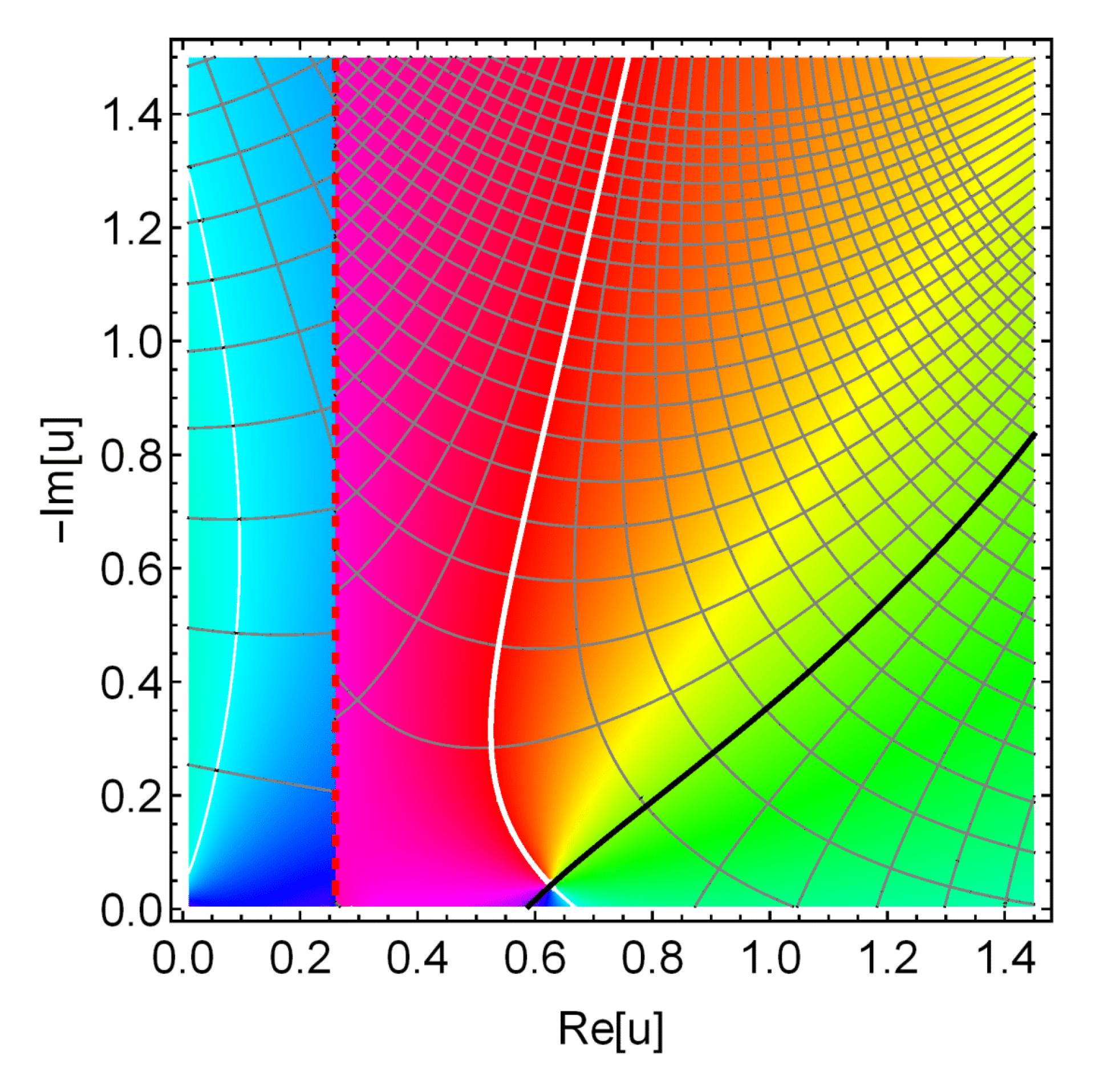
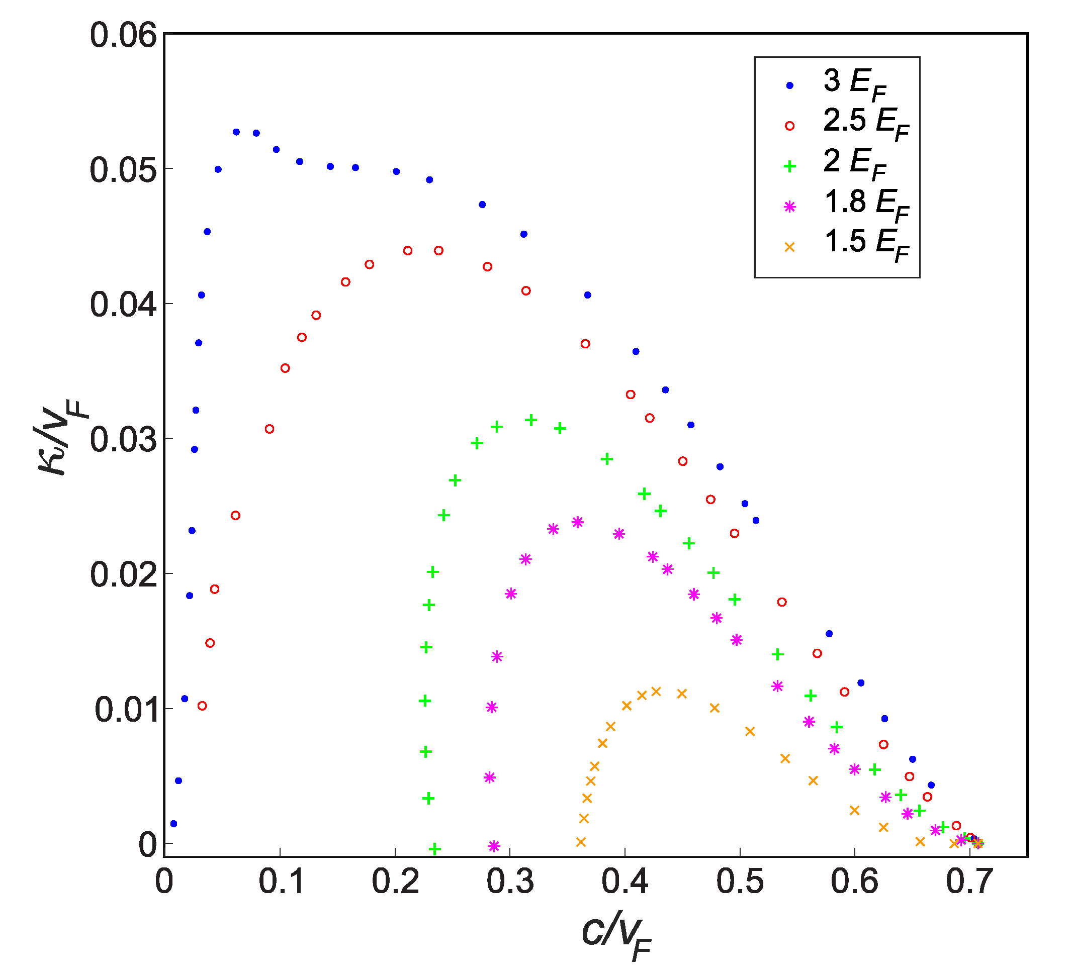
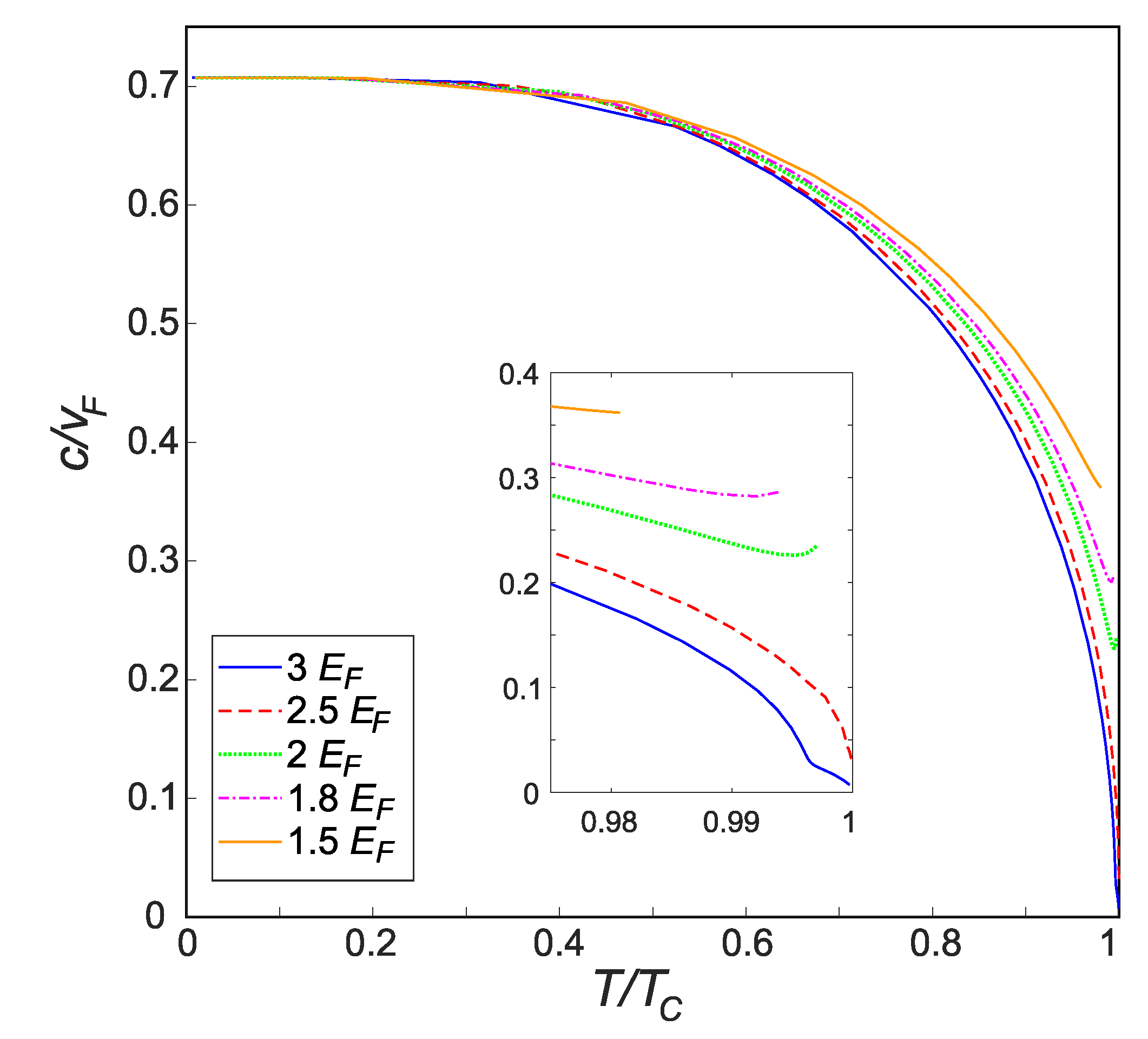
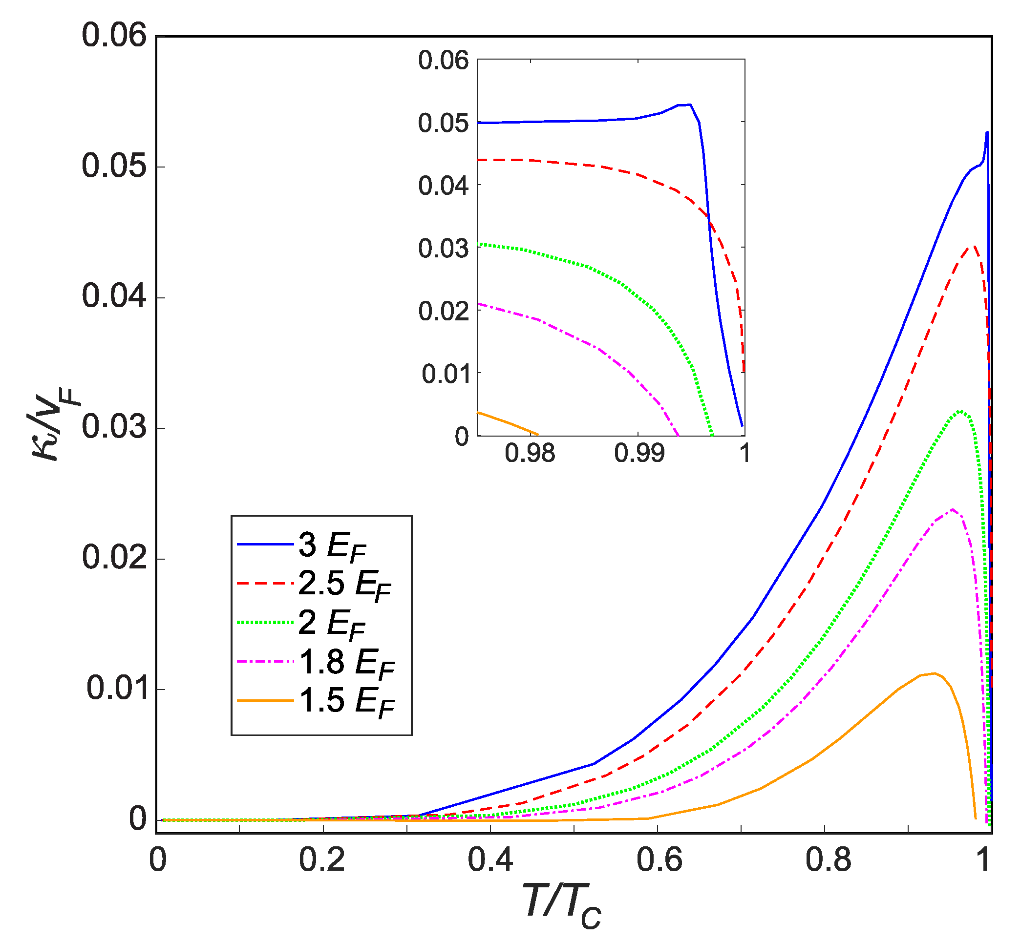
3.1. Sound Mode as Pole of the Propagator

In expressions (21)–(23) for the coefficients U, D and C, there are terms of the form

$$\mathcal{F}\left(u\right)={\int }_0^{\infty }\frac{f(k,u)}{\sqrt{u^2-v_k^2}}.$$

(24)

The denominator $\sqrt{u^2-v_k^2}$ results in a branch cuts along the real axis for $\mathcal{F}\left(u\right)$ in the complex u plane. As we need to obtain U, D and C in the lower complex plane to find solutions of (20), it is necessary to analytically continue these functions through the branch cuts. For this we use the same method as in Refs. [12,13], namely the analytic continuation scheme introduced by Nozières [26]. It is based on computing the spectral function along the real axis

$$\rho \left(c\right)=\frac{1}{2\pi i}\underset{\delta \to 0}{lim}\left[\mathcal{F}(c+i\delta )-\mathcal{F}(c-i\delta )\right].$$

(25)

Then in the lower complex plane, the continuation of $\rho$ provides the desired analytic continuation ${\mathcal{F}}^c=\mathcal{F}\left(u\right)+2\pi i\rho \left(u\right)$. The spectral function $\rho \left(c\right)$ exhibits a kink at $c=v_b$ satisfying

$$v_b=4\mu +6{\Delta }^2{\left(\mu {\Delta }^2+{\Delta }^2\sqrt{{\mu }^2+{\Delta }^2}\right)}^{-1/3}-6{\left(\mu {\Delta }^2+{\Delta }^2\sqrt{{\mu }^2+{\Delta }^2}\right)}^{1/3}.$$

(26)

The analytic continuation of the spectral function to the left of the kink is different from the continuation of the function to the right of $v_b$. This divides the analytically continued functions in two, as it effectively rotates the branch cut to the line $[v_b-0i,v_b-i\infty ]$. Hence, there are two regions in the lower complex u plane: domain I with $Re\left(u\right)<v_b$ and domain II with $Re\left(u\right)>v_b$. As in the three-dimensional case, the presence of the two domains has a physical origin: the group velocity $v_k$ corresponds to a Landau critical velocity for emitting fermionic excitations in the superfluid, and $v_b$ is the maximal group velocity for fermionic excitations with $k<k_F$. For more details on the continuation scheme (in 3D), we refer to [13].

An example of the analytic continuation is shown in Figure 1, plotting the numerically computed values of $det\mathbb{M}$ in the lower complex plane. A complex root is present at the point where the white line (where $Im\left(det\mathbb{M}\right)=0$) and the black line (where $Re\left(det\mathbb{M}\right)=0$) cross. This root corresponds to the complex sound velocity at the chosen parameters. The vertical red dotted line is the aforementioned branch cut between the two domains. The roots were always sought with an imaginary value of less than 2, because for higher values of $Im\left(u\right)$ the collective excitations are overdamped.

Changing parameters such as the temperature, we can track how the root of $det\mathbb{M}$ moves across the complex plane. Figure 2 shows the paths of the complex sound velocity u when the temperature passes from zero to $T_c$, the critical temperature at which $\Delta \to 0$. Various paths for u in the complex plane are shown, corresponding to five different values for the binding energy. At $T=0$ the results for all binding energies coincide at $u=v_F/\sqrt{2}$. This result has been obtained using the mean-field equation of state combined with the mean-field gap equation for background parameters $\left(\mu ,\Delta \right)$. The obtained zero-temperature sound velocity reproduces the known zero-temperature limit [27,28] which gives the constant sound velocity in 2D at all coupling strengths. This can also be shown analytically by taking the $\beta \to \infty$ limit in expressions (21)–(23). For non-zero temperatures, however, the sound velocity differs from the zero-temperature limit. Also taking into account fluctuations beyond the mean-field solutions changes the dependence of the sound velocity on the coupling strength even at zero temperature, so that it is not constant [29]. The present work is focused on the temperature dependence of the sound velocity and damping. Taking into account fluctuations is beyond the scope of this study.

As the temperature is increased towards $T_c$ the paths ends up on the real axis. In the BCS regime, the complex sound velocity disappears below the real axis before the critical temperature is reached. The path for $E_b=3E_F$ differs from the other paths due to the “bump” at the peak that we could not yet interpret. In general, a higher binding energy gives a higher damping rate, which is possible because the system in the BEC regime is more dependent on the temperature.

Figure 3 and Figure 4 show the temperature dependence of the sound velocity $c=Re\left(u\right)$ and the damping parameter $\kappa =-Im\left(u\right)$, respectively. Please note that $\kappa$ equals the damping rate divided by q—just as the energy, the damping rate is linear in q in the long-wavelength limit. The sound velocity decreases monotonically from its zero-temperature value of $v_F/\sqrt{2}$, but does not reach zero as the temperature reaches the critical temperature.

The general decreasing behavior of the sound velocity of a superfluid Fermi gas when the temperature rises from zero to $T_c$ is common both for 2D and 3D Fermi gases [10]. To understand better the dependence of the sound velocity in 2D on the binding energy and temperature, we can remind that the mean-field result for the sound velocity has been re-derived in Reference [28] using simple thermodynamic relation, which in the chosen units reads:

$$u=\sqrt{2n{\left(\frac{\partial \mu }{\partial n}\right)}_{L^2,T}}.$$

(27)

In the mean-field approach, the chemical potential at $T=0$ is [28]

$$\mu =E_F-\frac{1}{2}{E}_b=2\pi n-\frac{1}{2}{E}_b.$$

(28)

The chemical potential appears then to be independent on the binding energy and gives the aforesaid sound velocity $u=v_F/\sqrt{2}$ in the whole range of $E_b$. This is specific for a 2D gas, as distinct from 3D. Moreover, this result coincides with the zero-temperature sound velocity for an ideal Fermi gas in 2D, which is consistent with the BCS limit of a vanishingly small coupling strength. In the far BCS regime $k_B{T}_c\ll E_F$, hence the chemical potential and the sound velocity behave asymptotically close to their zero-temperature expressions. This explains why the decrease of the sound velocity as a function of the temperature becomes less expressed for weaker coupling strengths as can be seen from Figure 3.

The smaller the damping parameter $\kappa$ is, the more stable the collective excitations are, so that at $T=0$ we have fully stable excitations. As the temperature rises, as expected, $\kappa$ also rises, and when the temperature continues to rise, $\kappa$ goes down again. In the BEC regime, this result makes sense, since one must view $\kappa$ relative to c and if $\kappa$ tends to zero, c also goes to zero. The result that one gets in the BCS regime on the other hand is unexpected, namely a stabilization of the mode close to $T_c$. This may mean that our description of the system is not accurate at temperatures close to $T_c$ and that the present GPF approximate action for the 2D system is should be restricted to temperatures well below $T_c$. To get a better estimate of the regime of validity, we investigate the response function in the next subsection.

3.2. Response Function

An alternative way to determine the sound velocity, without relying on the analytical continuation, consists of using instead the response function. For low momentum, the pair field response function is given by [13]:

$$q^2{\mathbb{M}}^{-1}\left(uq,\mathbf{q}\right)=\frac{1}{U\left(u\right)C\left(u\right)-D{\left(u\right)}^2}\left(\begin{array}{cc}C\left(u\right)q^2& iD\left(u\right)q\\ -iD\left(u\right)q& U\left(u\right)\end{array}\right)+O\left(q^4\right).$$

(29)

The dominating term here is proportional to the phase-phase element ${\left({\mathbb{M}}^{-1}\right)}_{2,2}$. We determine the phase-phase response function in the long-wavelength limit as

$$\chi \left(c\right)=\underset{q\to 0}{lim}\frac{1}{\pi }Im\left[q^2{\left({\mathbb{M}}^{-1}\right)}_{2,2}\left(\left(c+0^{+}i\right)q,\mathbf{q}\right)\right]=\frac{1}{\pi }Im\left[\frac{U}{UC-D^2}\left(c+0^{+}i\right)\right]$$

(30)

Please note that a presence just below the real axis of a pole (i.e., a node of $UC-D^2$) will lead to a peak of $\chi \left(c\right)$. The location of the peak approximates the real value of the pole, i.e., to the sound velocity. The height of the peak is determined by the residue, and its width is determined by how far in the lower half plane the pole lies. Hence, the value of c for which the response function achieves a maximum $c\equiv c_{resp}$ can be used as an approximation for the sound velocity.

The numerical solutions for c and $c_{resp}$ lie close to each other, as can be seen from Figure 5. An advantage of this second technique is that it is more reliable to determine the sound speeds close to $T_c$, and hence allows us to estimate the region of validity for our results. From Figure 5, it can be seen that the sound speed starts to rise again close to $T_c$ in the BCS regime. This phenomenon is not intuitively expected and deviates from that of Figure 3 but can possibly be explained by second sound. The first sound is the sound wave of the density fluctuations. Normally, temperature differences spread through diffusion, but with second sound we have temperature fluctuations that behave like waves. Second sound only occurs in the Bose condensed state, so it is possible that in the BCS regime the first sound dominates and therefore does not disappear at and above the critical temperature, whereas the BEC regime second sound dominates and therefore disappears at $T_c$. Regardless of this interpretation, we can identify the region where c corresponds to $c_{resp}$ as the region where the method of finding the sound velocity from the poles of the bosonic fluctuation propagator is reliable. This turns out to be a rather large fraction of the temperature range, $T⪅0.95$ $T_c$.

4. Conclusions

The aim of this work is to determine the long-wavelength dispersion of Anderson–Bogoliubov excitations for two-dimensional superfluid Fermi gases by locating the poles of the propagator of pair field fluctuations. The fluctuation propagator is in turn obtained via an expansion of the matrix elements of the GPF action up to the second order in powers of q. As was the case for the 3D system, our method of analytical continuation does not need to assume that the poles lie close to the real axis (i.e., that the damping can be tackled perturbatively). We found that at $T=0$, the sound velocity is equal to $v_F/\sqrt{2}$ independently on the binding energy, being in line with preceding works, and the damping rate is equal to zero. For non-zero temperatures, the sound velocity differs from this known value. As the temperature rises, the sound velocity decreases and the damping increases. Taking into account fluctuations can of course change the dependence of the sound velocity and damping on the binding energy and temperature. For $T=0$ fluctuations can be included in the treatment rigorously, their influence on the equation of state of a Fermi gas in 2D at non-zero temperatures is a nontrivial problem, because the superfluid state in two dimensions is a quasicondensate rather than a true condensate. This is a subject of the future investigation.

The response function has been calculated for various temperatures and binding energies. The maxima of the response functions could then be used to determine the sound rates at different temperatures and binding energies in an alternative way, which gives almost the same results as those obtained through complex poles of the fluctuation propagator, except the close vicinity of the transition temperature, where the second method is more reliable. The estimated sound velocities agree with the previous results, and we get a better view at the sound velocity near the critical temperature $T_c$. In the BCS regime, we still have stable collective excitation at $T_c$, while in the BEC regime this is not the case. The reason for this could be that in the BCS regime first sound dominates and keeps existing past $T_c$, while in the BEC regime second sound dominates and disappears past $T_c$.

Recently, the sound mode was studied experimentally for a uniform Fermi superfluid in a box trap [7,8]. The superfluid was excited at a given frequency by vibrating a wall of the container, and the resulting density response was measured to estimate both the dispersion and the damping. A similar technique could well be employed to study the sound mode in the two-dimensional case, given the versatility of trapping potentials that can be achieved. This could allow experimental verification of the results predicted here. The straightforward extension of the present approach to Fermi gases confined to a frequently used parabolic confinement potential is possible for sufficiently large potential wells. In this case, a change of the sound velocity and damping comes completely from a renormalization of the gap and number equations in a trap [18,19,20] with respect to bulk. In the opposite case of a relatively small-radius confinement potential, the hydrodynamic approach used in Reference [20] can effectively determine spectra of discrete low-lying modes. Another promising development of the present study is related to the collective modes in ultra-cold Fermi gases with dipolar interactions intensely investigated recently [30,31,32]. Different interaction potentials, as well as a deformation of the Fermi surface [32] can be straightforwardly incorporated in the GPF approach. Finally, we note that the path-integral technique used here has as a specific advantage over some other methods that it explicitly allows the studying of damped collective modes at non-zero temperatures, relevant to the experiments.

References

1. Bartenstein, M.; Altmeyer, A.; Riedl, S.; Jochim, S.; Chin, C.; Denschlag, J.H.; Grimm, R. Collective Excitations of a Degenerate Gas at the BEC-BCS Crossover. Phys. Rev. Lett. 2004, 92, 203201. [Google Scholar] [CrossRef] [PubMed] [Green Version]
2. Kinast, J.; Turlapov, A.; Thomas, J.E. Damping of a Unitary Fermi Gas. Phys. Rev. Lett. 2005, 94, 170404. [Google Scholar] [CrossRef] [PubMed]
3. Altmeyer, A.; Riedl, S.; Kohstall, C.; Wright, M.J.; Geursen, R.; Bartenstein, M.; Chin, C.; Hecker Denschlag, J.; Grimm, R. Precision Measurements of Collective Oscillations in the BEC-BCS Crossover. Phys. Rev. Lett. 2007, 98, 040401. [Google Scholar] [CrossRef] [Green Version]
4. Tey, M.K.; Sidorenkov, L.A.; Guajardo, E.R.S.; Grimm, R.; Ku, M.J.; Zwierlein, M.W.; Hou, Y.H.; Pitaevskii, L.; Stringari, S. Collective Modes in a Unitary Fermi Gas across the Superfluid Phase Transition. Phys. Rev. Lett. 2013, 110, 055303. [Google Scholar] [CrossRef] [Green Version]
5. Sidorenkov, L.A.; Tey, M.K.; Grimm, R.; Hou, Y.H.; Pitaevskii, L.; Stringari, S. Second sound and the superfluid fraction in a Fermi gas with resonant interactions. Nature 2013, 498, 78. [Google Scholar] [CrossRef]
6. Hoinka, S.; Dyke, P.; Lingham, M.G.; Kinnunen, J.J.; Bruun, G.M.; Vale, C.J. Goldstone mode and pair-breaking excitations in atomic Fermi superfluids. Nat. Phys. 2017, 13, 943. [Google Scholar] [CrossRef] [Green Version]
7. Patel, P.B.; Yan, Z.; Mukherjee, B.; Fletcher, R.J.; Struck, J.; Zwierlein, M.W. Universal Sound Diffusion in a Strongly Interacting Fermi Gas. arXiv 2019, arXiv:1909.02555. [Google Scholar]
8. Mukherjee, B.; Yan, Z.; Patel, P.B.; Hadzibabic, Z.; Yefsah, T.; Struck, J.; Zwierlein, M.W. Homogeneous Atomic Fermi Gases. Phys. Rev. Lett. 2017, 118, 123401. [Google Scholar] [CrossRef] [Green Version]
9. Anderson, P.W. Random-Phase Approximation in the Theory of Superconductivity. Phys. Rev. 1958, 112, 1900. [Google Scholar] [CrossRef]
10. Ohashi, Y.; Griffin, A. Superfluidity and collective modes in a uniform gas of Fermi atoms with a Feshbach resonance. Phys. Rev. A 2003, 67, 063612. [Google Scholar] [CrossRef] [Green Version]
11. Combescot, R.; Kagan, M.Y.; Stringari, S. Collective mode of homogeneous superfluid Fermi gases in the BEC-BCS crossover. Phys. Rev. A 2006, 74, 042717. [Google Scholar] [CrossRef] [Green Version]
12. Kurkjian, H.; Klimin, S.N.; Tempere, J.; Castin, Y. Pair-Breaking Collective Branch in BCS Superconductors and Superfluid Fermi Gases. Phys. Rev. Lett. 2019, 122, 093403. [Google Scholar] [CrossRef] [PubMed] [Green Version]
13. Klimin, S.N.; Tempere, J.; Kurkjian, H. Phononic collective excitations in superfluid Fermi gases at nonzero temperatures. Phys. Rev. A 2019, 100, 063634. [Google Scholar] [CrossRef] [Green Version]
14. Klimin, S.N.; Kurkjian, H.; Tempere, J. Leggett collective excitations in a two-band Fermi superfluid at finite temperatures. New J. Phys. 2019, 21, 113043. [Google Scholar] [CrossRef]
15. De Melo, C.S.; Randeria, M.; Engelbrecht, J.R. Crossover from BCS to Bose superconductivity: Transition temperature and time-dependent Ginzburg-Landau theory. Phys. Rev. Lett. 1993, 71, 3202. [Google Scholar] [CrossRef] [PubMed]
16. Engelbrecht, J.R.; Randeria, M.; Melo, C.S. BCS to Bose crossover: Broken-symmetry state. Phys. Rev. B 1997, 55, 15153. [Google Scholar] [CrossRef]
17. Diener, R.B.; Sensarma, R.; Randeria, M. Quantum fluctuations in the superfluid state of the BCS-BEC crossover. Phys. Rev. A 2008, 77, 023626. [Google Scholar] [CrossRef] [Green Version]
18. Adhikari, S.K.; Salasnich, L. Superfluid Bose-Fermi mixture from weak coupling to unitarity. Phys. Rev. A 2008, 78, 043616. [Google Scholar] [CrossRef] [Green Version]
19. Gautam, S.; Adhikari, S.K. Weak coupling to unitarity crossover in Bose-Fermi mixtures: Mixing-demixing transition and spontaneous symmetry breaking in trapped systems. Phys. Rev. A 2019, 100, 023626. [Google Scholar] [CrossRef] [Green Version]
20. Klimin, S.N.; Tempere, J.; Devreese, J.T.; Van Schaeybroeck, B. Collective modes of an imbalanced trapped Fermi gas in two dimensions at finite temperatures. Phys. Rev. A 2011, 83, 063636. [Google Scholar] [CrossRef]
21. Feynman, R.P.; Hibbs, A.R.; Styer, D.F. Quantum Mechanics and Path Integrals; McGraw-Hill: New York, NY, USA, 1965. [Google Scholar]
22. Randeria, M.; Duan, J.M.; Shieh, L.Y. Superconductivity in a two-dimensional Fermi gas: Evolution from Cooper pairing to Bose condensation. Phys. Rev. B 1990, 41, 327. [Google Scholar] [CrossRef] [PubMed]
23. Hubbard, J. Calculation of Partition Functions. Phys. Rev. Lett. 1959, 3, 77. [Google Scholar] [CrossRef]
24. Stratonovich, R.L. On a method of calculating quantum distribution functions. In Soviet Physics Doklady; American Institute of Physics: College Park, MD, USA, 1957; Volume 2, p. 416. [Google Scholar]
25. Tempere, J.; Devreese, J.P. Path-Integral Description of Cooper Pairing. In Superconductors—Materials, Properties and Applications; Gabovich, A., Ed.; Institute of Physics: London, UK, 2012. [Google Scholar] [CrossRef] [Green Version]
26. Nozières, P. Le problème à N corps: Propriétés générales des gaz de fermions; Dunod: Paris, France, 1963. [Google Scholar]
27. Marini, M.; Pistolesi, F.; Strinati, G.C. Evolution from BCS superconductivity to Bose condensation: Analytic results for the crossover in three dimensions. Eur. Phys. J. B 1998, 1, 151. [Google Scholar] [CrossRef] [Green Version]
28. Salasnich, L.; Marchetti, P.A.; Toigo, F. Superfluidity, sound velocity, and quasicondensation in the two-dimensional BCS-BEC crossover. Phys. Rev. A 2013, 88, 053612. [Google Scholar] [CrossRef] [Green Version]
29. Bighin, G.; Salasnich, L. Finite-temperature quantum fluctuations in two-dimensional Fermi superfluids. Phys. Rev. B 2016, 93, 014519. [Google Scholar] [CrossRef] [Green Version]
30. Chan, C.K.; Wu, C.; Lee, W.C.; Sarma, S.D. Anisotropic-Fermi-liquid theory of ultracold fermionic polar molecules: Landau parameters and collective modes. Phys. Rev. A 2010, 81, 023602. [Google Scholar] [CrossRef] [Green Version]
31. Mulkerin, B.C.; Liu, X.J.; Hu, H. Leggett mode in a two-component Fermi gas with dipolar interactions. Phys. Rev. A 2019, 99, 023626. [Google Scholar] [CrossRef] [Green Version]
32. Veljić, V.; Pelster, A.; Balaž, A. Stability of quantum degenerate Fermi gases of tilted polar molecules. Phys. Rev. Res. 2019, 1, 012009. [Google Scholar] [CrossRef] [Green Version]
Figure 1. The (complex) determinant of the inverse fluctuation propagator is shown as a function of u, for E b = 1.8 and β = 0.87 . The color reveals the phase (along a color wheel from red over the spectrum to violet and then back to red). Curves show contours of the real and imaginary values.
Condensedmatter 05 00013 g001
Figure 2. Paths traced by the complex sound velocity when varying temperature from zero to the critical temperature, for different binding energies E b = 1.5 , 1.8 , 2 , 2.5 , 3 ( E F ) .
Condensedmatter 05 00013 g002
Figure 3. Sound velocity c as a function of temperature for E b = 1.5 , 1.8 , 2 , 2.5 , 3 E F .
Condensedmatter 05 00013 g003
Figure 4. Damping factor κ as a function of temperature for E b = 1.5 , 1.8 , 2 , 2.5 , 3 E F .
Condensedmatter 05 00013 g004
Figure 5. Sound velocity c r e s p as a function of temperature for E b = 1.5 , 1.8 , 2 , 2.5 , 3 E F . Inset: this sound velocity for temperatures close to T C .
Condensedmatter 05 00013 g005