Open-Source Digitally Replicable Lab-Grade Scales


1
Department of Mechanical Engineering–Engineering Mechanics, Michigan Technological University, Houghton, MI 49931, USA
2
Department of Electrical & Computerfigure Engineering, Michigan Technological University, Houghton, MI 49931, USA
3
Department of Material Science & Engineering, Michigan Technological University, Houghton, MI 49931, USA
4
Department of Electronics and Nanoengineering, School of Electrical Engineering, Aalto University, FI-00076 Espoo, Finland
*
Author to whom correspondence should be addressed.
Instruments 2020, 4(3), 18; https://doi.org/10.3390/instruments4030018
Submission received: 26 April 2020
/
Revised: 25 June 2020
/
Accepted: 25 June 2020
/
Published: 27 June 2020
Abstract
:This study provides designs for a low-cost, easily replicable open-source lab-grade digital scale that can be used as a precision balance. The design is such that it can be manufactured for use in most labs throughout the world with open-source RepRap-class material extrusion-based 3-D printers for the mechanical components and readily available open-source electronics including the Arduino Nano. Several versions of the design were fabricated and tested for precision and accuracy for a range of load cells. The results showed the open-source scale was found to be repeatable within 0.05 g with multiple load cells, with even better precision (0.005 g) depending on load cell range and style. The scale tracks linearly with proprietary lab-grade scales, meeting the performance specified in the load cell data sheets, indicating that it is accurate across the range of the load cell installed. The smallest load cell tested (100 g) offers precision on the order of a commercial digital mass balance. The scale can be produced at significant cost savings compared to scales of comparable range and precision when serial capability is present. The cost savings increase significantly as the range of the scale increases and are particularly well-suited for resource-constrained medical and scientific facilities.
1. Introduction
The incredible success of free and open-source development of software [1,2] is being rapidly adopted by the hardware community [3,4] as it enables scientific equipment designers to rapidly build upon one another’s work [5,6,7]. This has resulted in a democratization of design building on open-source designs [8,9,10] often with open-source tools that enable a true digital distributed manufacturing [11,12,13,14]. The most robust examples, is the self-replicating rapid prototype (RepRap) fused filament fabrication (FFF)-based 3-D printer [15,16,17] that has brought the cost of both rapid prototyping and additive manufacturing low enough to be used by the masses [18,19,20,21]. FFF-based 3-D printers derived from RepRaps now have 3-D printed parts with sufficient mechanical strength [22] to be used for final functional parts even if printed on machines that only cost a few hundred dollars. This has resulted in an explosion of open-source digitally fabricated instruments and a repository of designs housed at the NIH [5,6,23,24]. There are many examples of progressively more sophisticated open-source 3-D printed parts being used to build chemical mixing systems [22,23,24,25], mechanical components for optics setups [26,27,28,29,30,31] and microscopes [32,33,34], instruments to test water quality testing [35,36,37,38], various types of syringe pumps [39,40,41,42,43] that are combined with other components to make complete systems for making microfluidics and metafluidics [44,45,46,47]. Although the most important features of open-source 3-D printable instruments is the ease with which scientists can customize a tool, in general, they are also much less expensive than equivalent (and often technically inferior) commercial proprietary systems [6,23,24,48,49,50] and provide a high return on investment [51,52]. This advantage expands as the device is made with a higher percentage of digitally replicable components [53]. To continue this tradition of standing on the shoulders of open hardware giants [54], this paper describes the design of an open-source largely 3-D printed digital scale. A digital scale is a scientific instrument that provides fast measurements of mass generally with an accuracy range of 0.1 g to 0.01 g and have easy-to-read automatic liquid crystal displays. (Accuracy refers to closeness of the measurements to a known value of the mass. On the other hand, precision refers to the closeness of the measurements to one another, which is commonly stated as a single standard deviation of several tests and is independent of the accuracy (i.e., statistical dispersion).) Digital scales are used in a wide range of scientific applications including chemical research, genomics, drug discovery, and proteomics. Scales are classified by precision; where a precision balance has a measurement resolution of 0.001 g, an analytical balance has one of 0.0001 g and a micro balance has one of 0.0000001 g. On the high-end of scales, an open-source quartz crystal microbalance (OpenQCM) [55] uses an open-source Arduino Nano and is already well established in the scientific literature [56,57,58,59,60].
Thus, this study provides the designs for a low-cost, easily replicable, open-source lab-grade digital scale that can be used as a precision balance depending on configuration. The design is such that it can be manufactured for use in most labs throughout the world with open-source RepRap-class material extrusion-based 3-D printers for the mechanical components and readily available open-source electronics including the Arduino Nano. In addition, a validation procedure for quantifying the accuracy and precision is provided. Several versions of the design were fabricated and tested for a range of load cells, and the results are discussed in the context of resource-constrained medical and scientific facilities.
2. Materials and Methods
2.1. Design
This series of open-source scales is based on load cells, which are devices designed to measure weight or force. The load cells used in this study are strain gage load cells, which convert strain (i.e., change in length) of a material into an electrical signal proportional to the force applied [61]. This series of scales was designed to be easily manufacturable, require minimal components, and offer the functionality necessary for a basic digital scale, a precision balance, and an analytical balance. Component location is accomplished entirely by features on the 3-D printed components including bosses and snap-fit joints, meaning that the only fasteners required are those that hold the load cell in place. The assembly was designed to fully enclose all electronics, limiting airflow, which has been observed to affect the output of the load cell amplifier.
At the time of writing, the scale is designed to accommodate two sizes of single-point parallel beam load cells—TAL220 and TAL221—but is set up to enable fast adaptation to other models. These were selected first due to their low cost, wide selection of weight ranges, and insensitivity to moment loading on the bed, which aids in measurement repeatability [61]. The base and bed were designed to be easily modified to accommodate other load cell styles as required.
The open-source scale systems were designed for use in two settings: (1) as an independent digital scale with a displayed output which can be tared (the reference for a reading of zero can be offset to ignore a known mass, such as that of a container) and calibrated (the output can be corrected to present the true mass by loading the scale with a known mass) without use of a computer, and (2) as a serially connected logging instrument for a laboratory setting and data-logging. The serial capability also allows this scale to be constructed without an LCD, offering a significant cost reduction for uses that do not require a display, such as automated weighing or cases where a computer will always be used as the power supply.
To accomplish independent functionality, components were specified to ensure that the entire scale can be powered by a 5V USB power supply, either from a computer USB port or cell phone charging block, both of which are commonly available at low cost. The components’ power requirements are small enough that the low-current digital pins on an Arduino can power them, allowing independent control of power to each component, which is leveraged in the implementation of power-saving features [62,63,64]. The scale’s tare and calibration functions are controlled with a single push-button—pressed for tare, and held for several seconds to calibrate.
As a logging scale, the microcontroller is configured to interface serially with a computer. The API for serial communication is built to comply with the Scale Manufacturers Association (SMA) SCP-0499 Level #2 standard for limited-feature digital scale serial communication protocol. This includes capability to serially query the scale output, command tare, calibration, and provide basic scale information [65]. The API allows for continuous tracking of the scale readout for data-logging, which is useful for automated data-collection in cases such as long-term mass-tracking and discrete automated processes such as melt flow indexing (MFI).
2.2. Bill of Materials
The bill of materials (BOM) is shown in Table 1.
2.3. Manufacturing and Assembly
The 3-D printable components shown in Table 1 are available to be freely downloaded on the Open Science Framework (OSF) [81] and are released under a GNU General Public License (GPL) 3.0 [82]. All the required STL-rendered components were 3-D printed polylactic acid (PLA), filament of diameter 2.85 mm on a Lulzbot TAZ 6 (Aleph Objects, Loveland CO). The objects were sliced with Cura Lulzbot edition v.3.6.20 [83] using the settings detailed in Table 2. The optional cover was 3-D printed translucent glycol modified polyethylene terephthalate (PETG) filament of diameter 2.85 mm on a Lulzbot TAZ 6 [84].
After printing the components, all support material and brims were cleaned from the components. Please note that these components can all be printed without support material, depending on required surface finish.
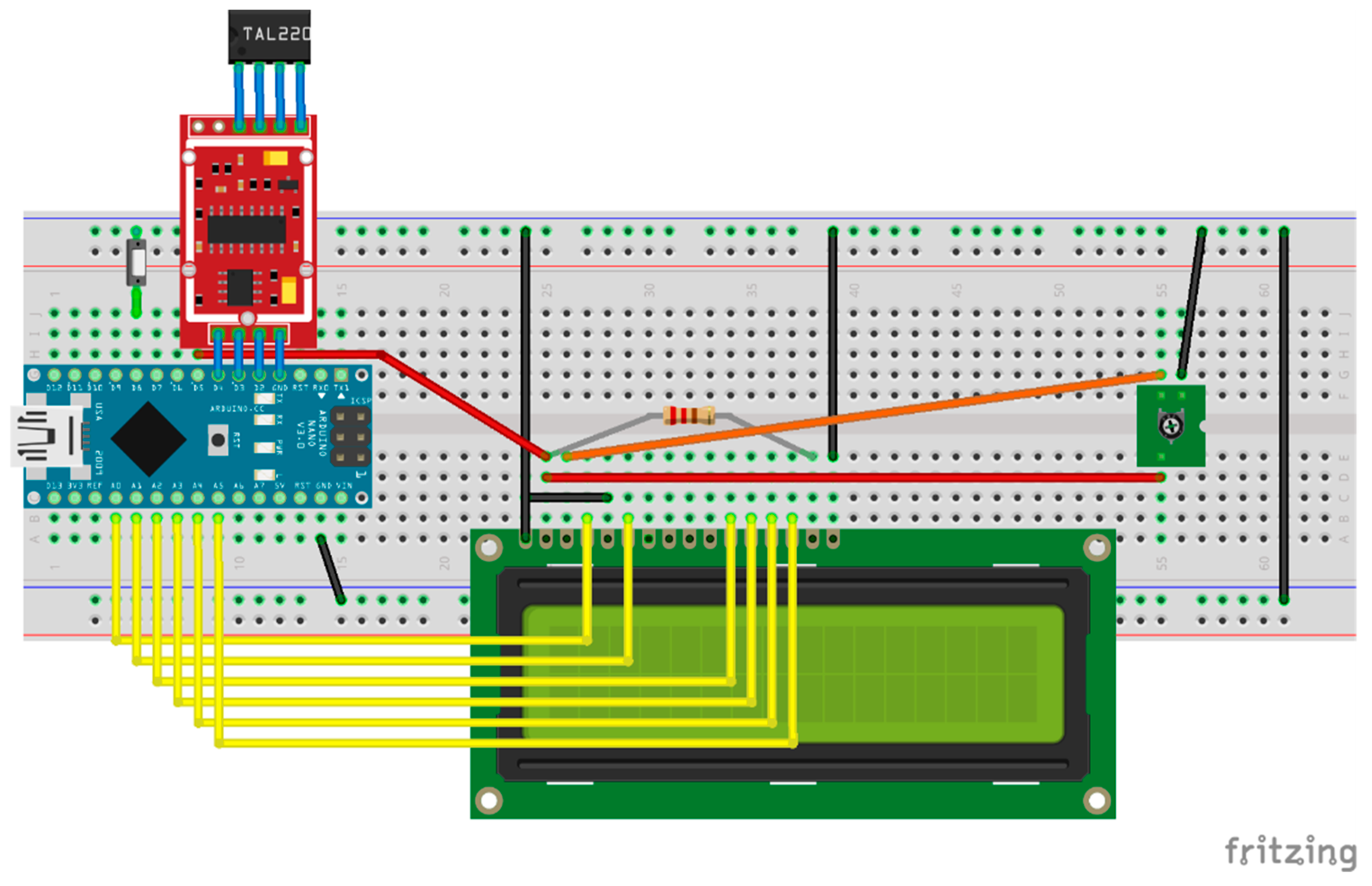
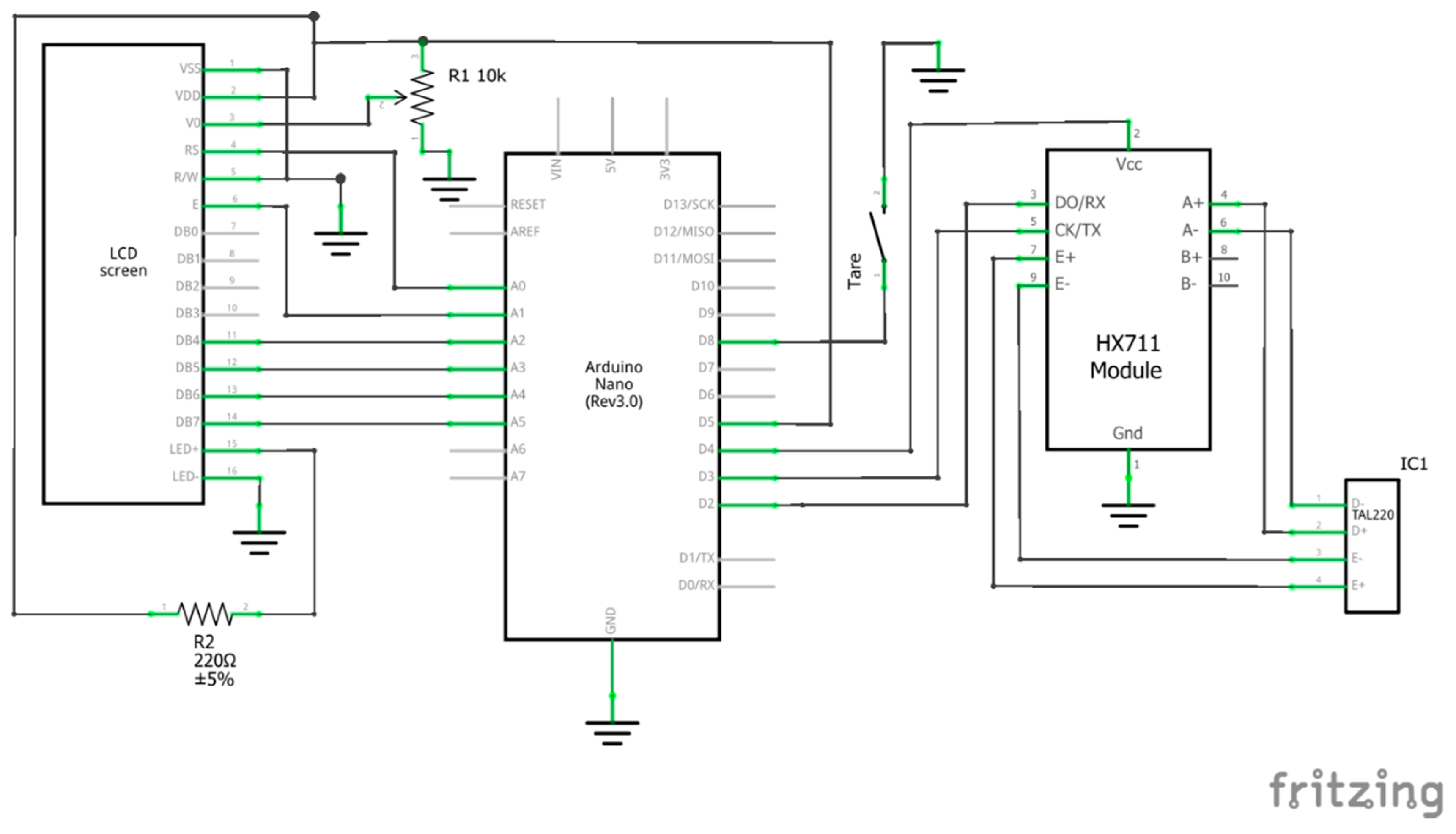
The electronics were assembled according to the diagrams in Figure 1 and Figure 2, which were created with Fritzing [85]. The LCD was wired based on Arduino documentation [86].
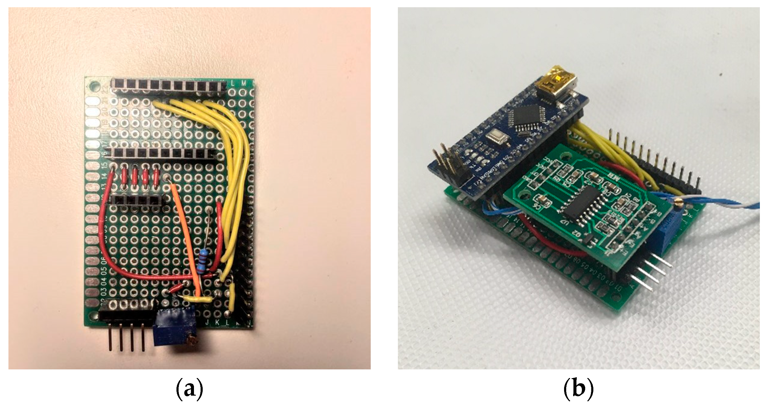
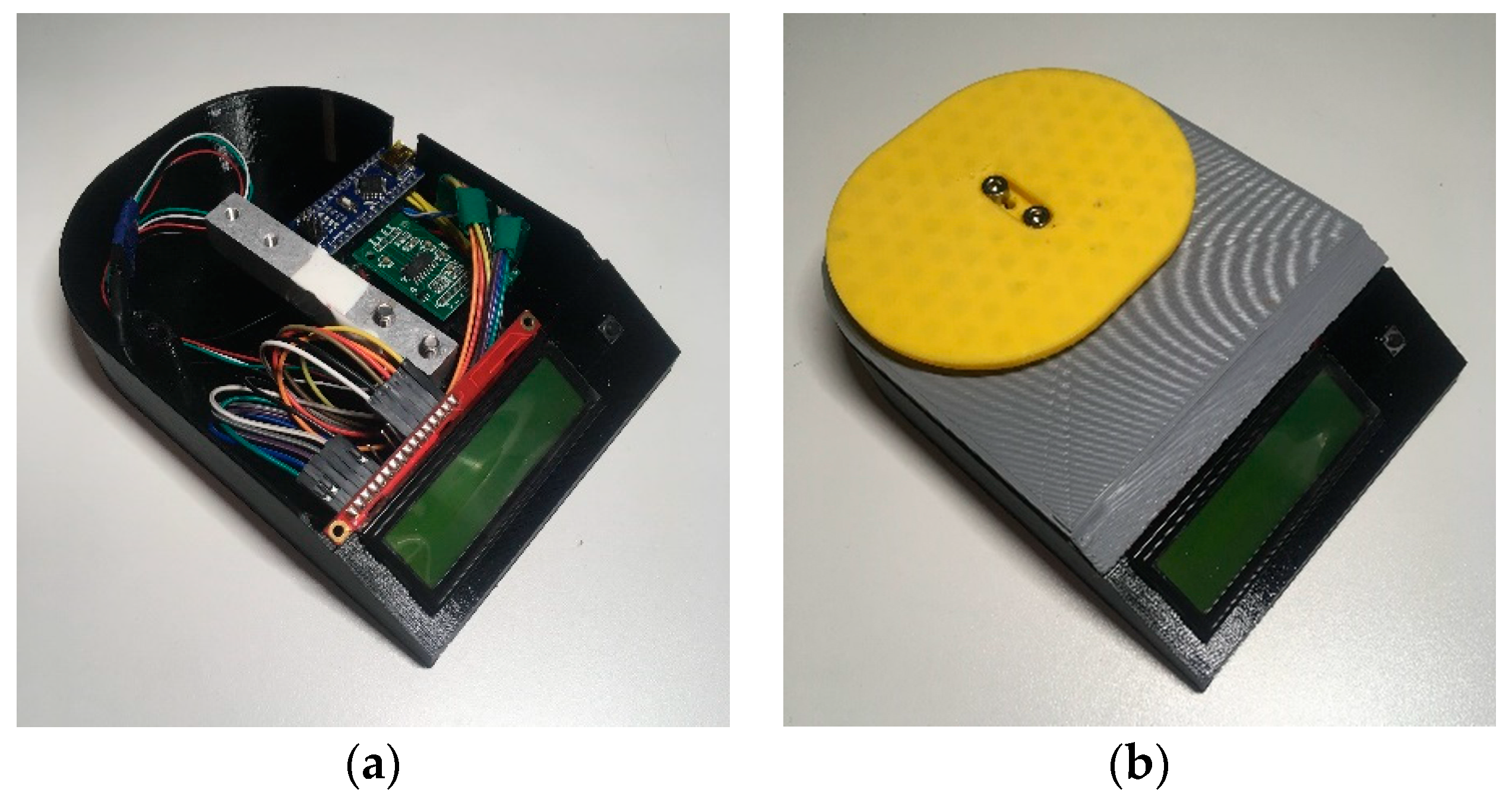
After verifying functionality with a solderless breadboard, the components were installed on a 40x60mm solder breadboard as shown in Figure 3. To install the tare button on the face of the scale, a twisted pair was connected to the button pinouts and the button not immediately connected. The button was not connected to the twisted pair until after assembly. To allow for interchange of the Arduino, the HX711, the LCD, and the load cell, these were connected with header pins and jumper wires. The Arduino was purposefully placed to align with the slot on the side of the 3-D printed base for USB access when fully assembled.
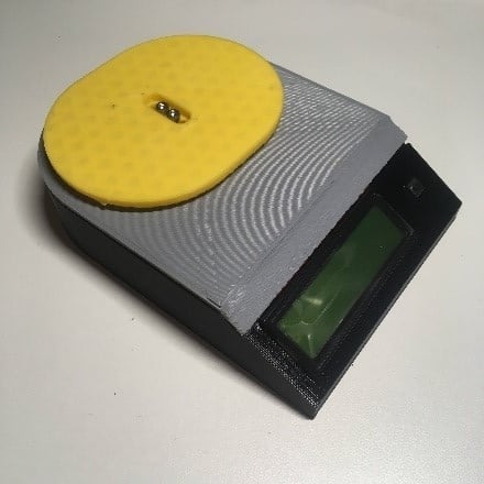
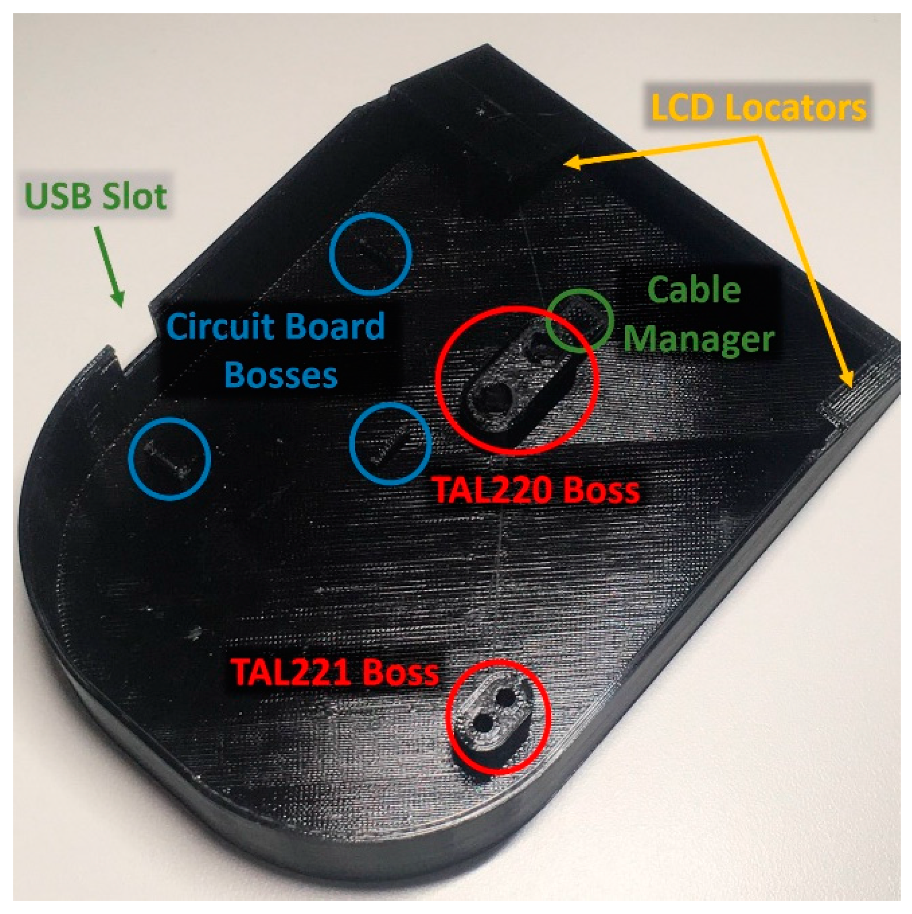
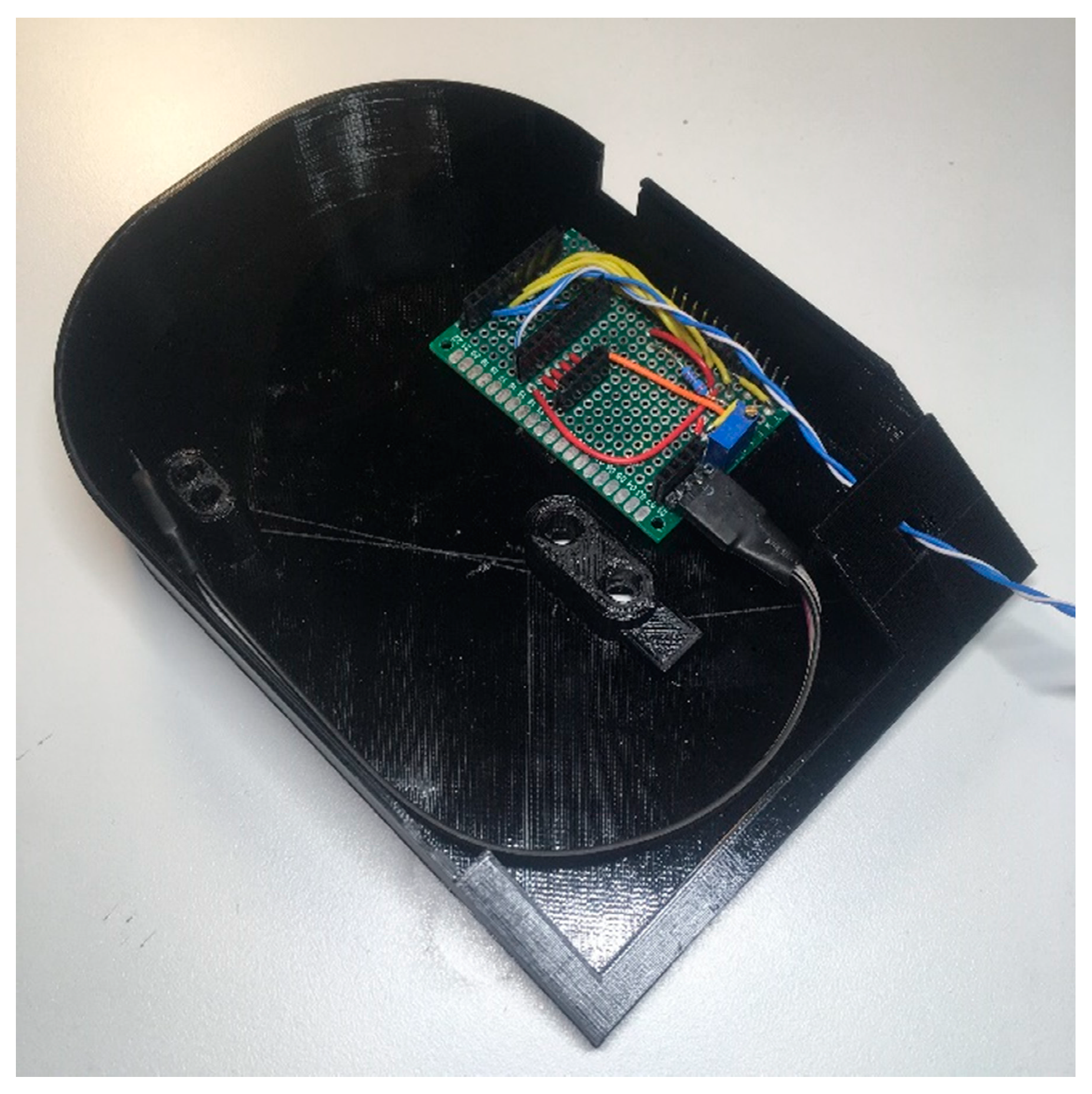
The 3-D printed base has several features to aid in assembly (Figure 4). The assembled circuit board was fit into the 3-D printed base—the base has bosses on the right side (facing the front) that locate the board and hold it in place when connecting and disconnecting a USB cable to the Arduino (Figure 5).
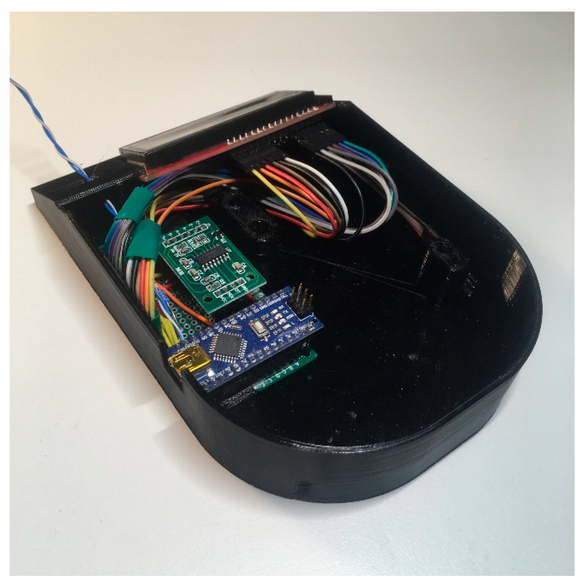
The Arduino and HX711 were attached to their respective header pins. The LCD was placed in the locator slots on the front of the scale. The wires for the LCD were tucked under the cable manager on the TAL220 boss, then connected to the headers on the circuit board (Figure 6). The cable manager ensures that the wires from the LCD do not contact the load cell, which would interfere with measurement accuracy.
At this point the scale was powered on to set the potentiometer, which controls the contrast on the LCD. This can be set and then left alone. To do this, the Arduino was connected to a computer with the DigitalMassBalance firmware via USB. After uploading the firmware, a serial connection was opened to monitor the output from the microcontroller. The output indicates whether the scale has initialized correctly, informing the user as devices are powered on and checked. The LCD continuously displays the measured mass once powered on. The potentiometer was adjusted until the readout (number and unit) were easily visible on the LCD. In cases that the display appears non-functional, it should be checked in low light—if the screen does not appear backlit, no power is reaching the LCD. If it is receiving power, one of the jumpers is likely loose and all connections should be checked. SparkFun’s LCD Hookup guide provides helpful and detailed troubleshooting suggestions if these checks do not work [87].
Prior to soldering the push-button in place, the lead wire connections to the controller should be checked. With the controller powered on, the tare is checked by shorting the twisted pair—a dot display on the bottom right of the LCD appears when the pair is shorted, indicating proper communication. With that checked, the button can then be soldered and secured in place. A small amount of non-conductive glue may be used to keep the button in place.
After setting up the LCD, the load cell was installed. The load cell must be mounted so that its wires run toward the base-fixed end of the load cell. The wires will interfere with measurement accuracy if running from the floating end of the load cell. The installation procedure depends on the load cell style in use:
- TAL220: Install the M5 end (the wires run to this end) to the TAL220 boss on the base of the scale (Figure 7). Connect the load cell to the HX711 pinouts—Red:E+, Black:E–, White:A–, Green:A+. Snap the cover onto the base—this fully encloses the electronics, offering some protection from thermal variations on the amplifier. Attach the bed to the load cell using the M4 bolts.
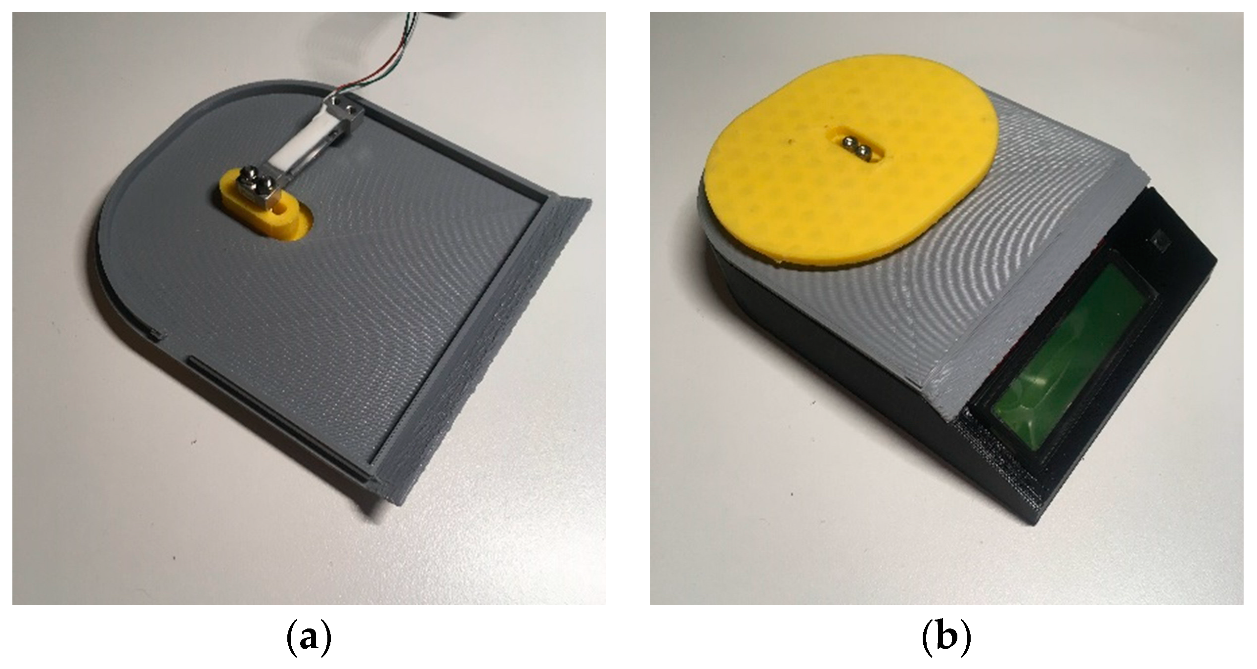
- TAL221: Sandwich the cover between the bed and the load cell. Connect the untapped end of the load cell (the wires do NOT run to this end) to the bed using M3 screws and nuts (Figure 8a). Connect the load cell to the HX711 pinouts—Red:E+, Black:E–, White:A–, Green:A+. Finally, attach the tapped M3 end to the TAL221 boss on the base (Figure 8b). This fit is tight so the wires on the load cell lead off the end fixed to the base.
2.4. Firmware
The firmware to drive the scale (called DigitalMassBalance) is also in the OSF repository [81]. A single installation contains functionality for both configurations of the scale (simple scale with digital display and lab scale with serial interface). The configuration header file, Config.hpp, can be modified to tell the controller whether an LCD is installed. Changing this setting determines whether the LCD will be initialized upon startup; and the serial interface listens by default as this has negligible effect on performance.
The firmware package makes use of two open-source libraries: (1) the HX711 library by GitHub user bogde [88], used under the MIT License; and (2) the LiquidCrystal Library for Arduino by Hans-Christoph Steiner [89], used under the GNU Lesser General Public License.
The HX711 library provides an interface with which to initialize, and read from, the HX711 load cell amplifier. The HX711 library can provide raw (long integer with tare offset) or calibrated (scaled by a sensitivity value from unitless integer to mass with units) data. The library’s built-in tare offset is used to implement zeroing of the scale (only the bed—no containers), while taring (subtracting a known mass from the reported value) is implemented in the firmware. Raw data is collected from the HX711 library to allow flexibility in the data averaging/filtering scheme used by the scale.
The LiquidCrystal library is used to write information to the LCD. Methods in the DigitalMassBalance firmware interface with the library, clearing the screen, moving the cursor, and writing information.
The DigitalMassBalance firmware itself is composed of a single Arduino source-code file, DigitalMassBalance.ino, which implements all methods and loops used during normal operation, plus three header files which organize definitions used by the firmware:
- Config.hpp contains configuration variables for the HX711, the LCD, and calibration and serial communication protocols.
- Libraries.hpp contains ‘#include’ statements for all the libraries used by DigitalMassBalance.
- Pinouts.hpp contains definitions for the location of hardware connections to the Arduino. These can be modified to accommodate the pinouts used in a particular setup.
Upon receiving power, the Arduino runs its setup loop, which completes six steps:
- Initialize a 9600 baud serial connection. The firmware is set to wait for serial communication to initialize before continuing. Please note that this does not noticeably affect startup time when receiving power from a non-serial-enabled device (such as a 5V power block or a battery).
- The HX711 undergoes a similar startup procedure, receiving power and ensuring proper communication. This is indicated by a series of readouts over serial.
- If an LCD is expected by the firmware (set in Config.hpp), the LCD is powered up. Once it is on, all digits of the display flash with the character ‘8’ for less than a second. This initialization is also indicated by readouts over serial.
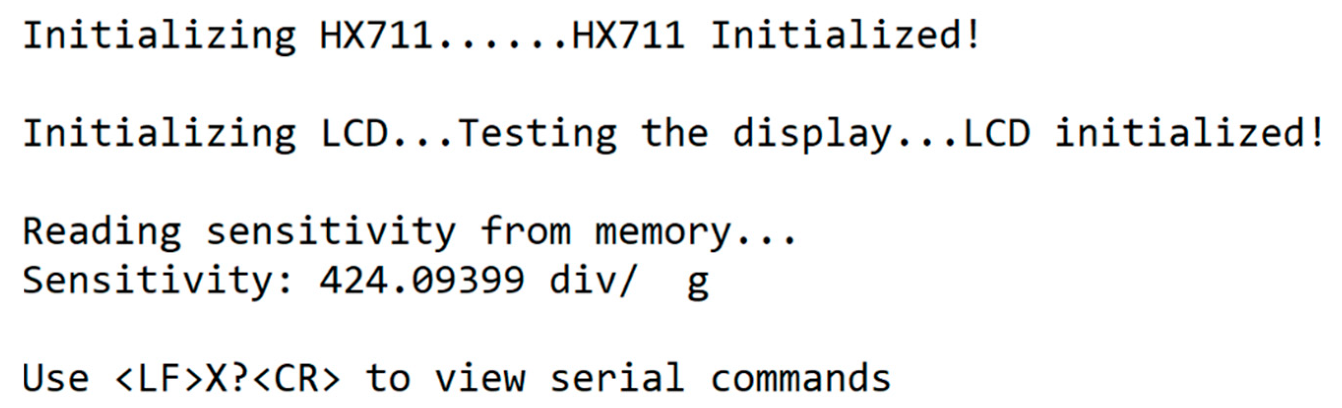
- With the hardware running, the Arduino checks its hard memory (EEPROM) for a saved calibration sensitivity (such a value is saved at the end of a calibration sequence). If one exists, the sensitivity is read and applied to the digital readout. If no sensitivity is saved, the scale defaults to a value of 1, which just returns the raw measurement from the HX711. The read sensitivity value is reported over serial. This message completes unsolicited responses from the scale—all further communication from the Arduino result from commands sent over serial. A complete, successful initialization is shown in Figure 9.
- At the time of writing, a simple averaging window is used to stabilize measurements from the scale. Measurements are stored in a first-in-first-out (FIFO) queue whose size is set in Config.hpp. The size of this window affects the response time of the scale. During initialization, this queue is automatically cleared to an array of zeros.
- Finally, the tare button is set to an input in INPUT_PULLUP mode, which makes use of an internal pullup resistor. This setting saves component cost and makes the tare button active LOW.
After completing setup, the Arduino enters a loop. With each iteration, the current mass measurement is retrieved from the HX711 and stored in the averaging queue, and the average mass is calculated and stored. This occurs as fast as the Arduino can process—there is no enforced sample rate for the mass. The Arduino also listens for serial input consistent with SMA SCP 0499 (detailed in Section 2.5.2, which discusses the operation of the scale as a lab scale) [65]. At the same time, it displays the current averaged mass measurement on the LCD and checks for a press of the tare button. These listening and reporting actions are completed at an enforced refresh rate (set in Config.hpp). This is done to visually stabilize (slow down) the LCD output and to enforce the rate at which data is reported over serial.
2.5. Operation of Design
The scale is designed for two forms of interaction: (1) as a simple scale with LCD output and push-button interaction and (2) as a lab scale with a serial interface to allow data-logging and advanced control of the scale. Both are discussed below as well as illustrated in ‘MOST OS Balance.mpeg’, a use video available on the OSF repository. Please refer to the Supplementary Materials.
2.5.1. Simple Scale
For simple use, the scale is connected to power over USB to a 5V power block, such as that used to charge a cellphone. Alternatively, 5V power can be provided to the Arduino 5V and Ground (GND) pins through other means. Possible interactions are:
- Tare: A press and release of the push-button on the front of the device will tare the scale to the current weight. The push-button is acknowledged when closed (pushed) by a dot on the lower right-hand corner of the LCD.
- Calibrate: Pressing and holding the push-button for at least 3 seconds (the wait time is adjustable in Config.hpp) will initialize a calibration sequence using the calibration mass set in Config.hpp. The scale will tare, then indicate the mass to apply to the bed. After detecting an added mass, the scale will measure the mass for 10 averages, then calculate the new scale sensitivity and save it to EEPROM.
2.5.2. Lab Scale with Serial Interface
The scale’s 9600 baud serial interface has been designed to Level #2 compliance with the SMA Scale Communication Protocols [65]. This includes the six specified Level #1 commands, plus additional commands. The full command list is detailed below, listing the command name, command character (indicated <char>), followed by a brief description where necessary. All command characters must follow a linefeed <LF> and precede a carriage-return <CR>. Full details of the response format and communication protocol are available in SMA SCP-0499 [65].
- Return displayed weight <W>.
- Zero the scale <Z>.
- Run scale diagnostics <D>. This is specified by SMA to check for memory or calibration errors.
- Return ‘about’ information for the scale <A>, <B>. These are specified by SMA to return information about the scale’s compliance level and firmware information.
- Reset the scale <ESC>.
- Continuously report weight <R>. Returns weight at the read rate until another command is received.
- Tare the scale <T>. This is different from zeroing in that the tare is for, as an example, ignoring the mass of a container. Meanwhile, zero is intended to set ‘zero’ for the scale with nothing on the bed.
- Clear the current tare <C>. This sets the tare weight to zero, causing further readouts to reference to the zero set by <Z>
- Return the tare weight <M>.
- Calibrate the scale <XC><xxxxxx.xxx> Enters a calibration cycle for the weight specified by <xxxxxx.xxx>. <XC> on its own may also be used to enter a calibration sequence using the default calibration mass set in Config.hpp
- Toggle power to the LCD <XL>. This changes the power state of the LCD, either turning it off or reinitializing it. This can be used for power savings when the display is not needed.
- Scroll output precision <XP>. This scrolls the number of digits on the readout between 0 and 4.
- List possible commands <X?>. This lists the recognized commands for the user. Since the leading X (required by SMA SCP 0499) is non-intuitive, it is indicated at the completion of the setup loop (Figure 9).
2.6. Validation
The 3-D printed open-source scale was tested against two proprietary laboratory-grade scales and with standard calibration weights, to check the functionality, accuracy, and linearity of the scale. The open-source scale was tested for three load cells: (1) a 5kg TAL220 load cell, (2) a 500 g TAL221 load cell and (3) a 100 g TAL221 load cell. TAL220 and TAL221 refer to the shape of the load cell. The mass range is determined by the size of the cutout in the middle of the load cell where less material left behind yields a more sensitive/lower mass range.
2.6.1. Laboratory-Grade Scale Comparison
The open-source scale was tested against a Denver APX402 400/0.01 g digital mass balance and a Denver A-160 160/0.1 mg digital analytical balance [90,91]. The A-160 was calibrated 2 months prior to the first round of testing. Due to limitations in the range of the two proprietary lab-grade balances, neither load cell was tested to the full range in this scale. The APX402 and the open-source scale were tested up to 300 g. The A-160 and the open-source scale TAL221 were tested up to 150 g. However, rigorous testing of the load cells themselves, was not the purpose of this testing—the results of such testing are documented in the manufacturer data sheets for load cells and the load cell amplifier [63,78,79].
To calibrate the scale, a container was measured on the A-160. Using the measured mass (reported down to 0.1mg) as a reference value, the scale was put into calibration mode. The scale tared itself, then waited for the reference mass to be added. Once added, the scale took a total of 100 averaged measurements over the span of several seconds in order to determine the sensitivity of the load cell (i.e., calibration value that multiplies a raw value to obtain a value with units).
The tests were completed using a light container with sand incrementally added. The container was placed on the APX402 scale, but not tared. Sand was added to the container until a desired mass was achieved. The container of sand was then massed on the APX402, the A-160, and the scale, in that order. After the upper limit of the A-160 was reached (160 g), the APX402 and open-source scale were still tested until the upper limit of the APX402 (around 330 g). The A-160 has a glass case, which was closed while taking measurements. The APX402 and the open-source scale did not have any cases to protect from airflow interference. Measurements were repeated 5 times for each increment of mass to check the repeatability of measurements (precision).
To compare the measurements among the three scales, two measures were computed. First is the standard deviation of the measurements at each discrete mass. This was computed for each individual scale to offer comparison on the stability of their readouts, indicating the precision of each instrument. Second, in an attempt to quantify the accuracy of the scale, its average measurement for each discrete mass up to 160 g was compared to the average measurement of the A-160 (the device used to calibrate it) using the absolute value of the difference between the two. The differences offer some perspective on how closely the open-source scale tracked with the proprietary lab-grade scales.
2.6.2. Self-Calibration of Open-Source Scale for 100 g TAL221
Often a developer of open hardware may only have access to a calibrated scale initially, so it is important to be able to calibrate the open-source scale from previous measurements (e.g., self-calibration). To demonstrate this the 100 g TAL221 was tested against the previously tested (calibrated) 500 g TAL221.
Four containers were filled to nominal masses of 25, 50, 75, and 100 g as measured on the 500 g TAL221. These new masses can be considered secondary standards as their masses are known to the accuracy of the 500 g TAL221. After measuring all 4 masses 5 times on the scale, the 100 g TAL221 was installed on the open-source scale. It was calibrated using the 75 g mass. All 4 masses were then measured 5 times on the 100 g TAL221. The resulting data was processed in the same manner as the other two tests, except average differences are referenced to the 500 g TAL221 load cell.
2.6.3. Measurement on Open-Source Scale Using Standard Masses
In a final set of tests to quantify the behavior of each load cell, the open-source scale was used to weigh a set of calibration weights (standard masses) ranging from 1 g up to 100 g, with rated accuracy of +/−0.005 g. The scale was set up with each load cell installed in the 3-D printed (PLA) housing and connected via USB to a computer. With the scale powered up, the electronics were allowed to warm up for at least one hour prior to calibration and testing.
The masses were handled using tweezers and stored in a plastic bag in between measurements to prevent contamination (which could affect the overall weight). The 100 g TAL221 was calibrated using a 20 g mass; the 500 g TAL221 and 5kg TAL220 were calibrated using a 100 g mass. The sensitivities used for each load cell were recorded with the raw data.
A PuTTY session was used to log data returned from the scale in continuous logging mode (command <R>). The scale was set to report an averaged weight at a report rate of 1 Hz. The average weight was calculated from a 10-value sliding average, sampled at an unregulated rate (however fast the processor could loop). This was observed to have a 10–90% rise time of 1 second. Each mass was placed on the scale and allowed to sit for around 30 seconds, returning between 23 and 48 measurements (depending on the actual time the mass was on the bed). Two complete datasets were gathered and averaged together, providing a minimum of 48 measurements for each mass on each load cell.
The standard deviation and average value of the logged data were calculated. The raw and processed data are stored in the OSF repository [81]. These results illustrate the scale’s behavior (statistical dispersion) without the influence of a human reading numbers from a display. It also gives a better indication of the accuracy of the scale since the masses are considered to be known.
To assess the influence of the plastic housing on the scale’s behavior, the 5kg TAL220 was re-tested while mounted to a simple frame made of two 1x6x6-inch (25x150x150 mm) common pine boards with spacers to float the load cell body above the pine, providing a fourth dataset for comparison.
2.7. Economic Analysis
To determine the costs of the various versions of the open-source digital scale, the 3-D printable components were massed on another digital scale +/−0.01 kg. The total cost (Tc) of the apparatus can be determined by
where V is the cost of the vitamins (or non-digitally manufactured components listed in Table 1), m is the mass of all the 3-D printed parts (e.g., all the STL-rendered parts in Table 1); Ce is the cost of the electricity per kg to print; and Cp is the cost of plastic per kg. The Lulzbot Taz 6 uses approximately 9.11 kWh per kg, as measured by a multimeter +/−0.01 kWh and reported previously [92]. The average cost of electricity in the U.S. is about $0.1029/kWh [93]. The cost of the PLA filament from Lulzbot was U.S. $20/kg [94].
3. Results
Two sets of testing were completed on the scale. These tested the scale under different conditions and offer different insights to the behavior of the scale.
The first set of tests compares the open-source scale with commercial scales. This set trusts the commercial scales to provide an accurate weight measurement, both for calibration and comparison. These tests exercise the repeatability of the scale when removing and re-adding weight to the scale. The measured mass was recorded by reading the value from the LCD, introducing room for human error during the test.
The second set of tests use only the open-source scale to measure standard calibration weights. This set trusts the weights to be accurate for calibration and for assessing the accuracy of the scale. The measured mass was recorded automatically via serial communication, providing a larger data set to illustrate the motion of the scale’s readout when at rest. Since the masses are assumed to be known, this set gives a better idea of the accuracy of the scale (within the limits of the accuracy of the masses themselves).
3.1. Laboratory-Grade Scale Comparison
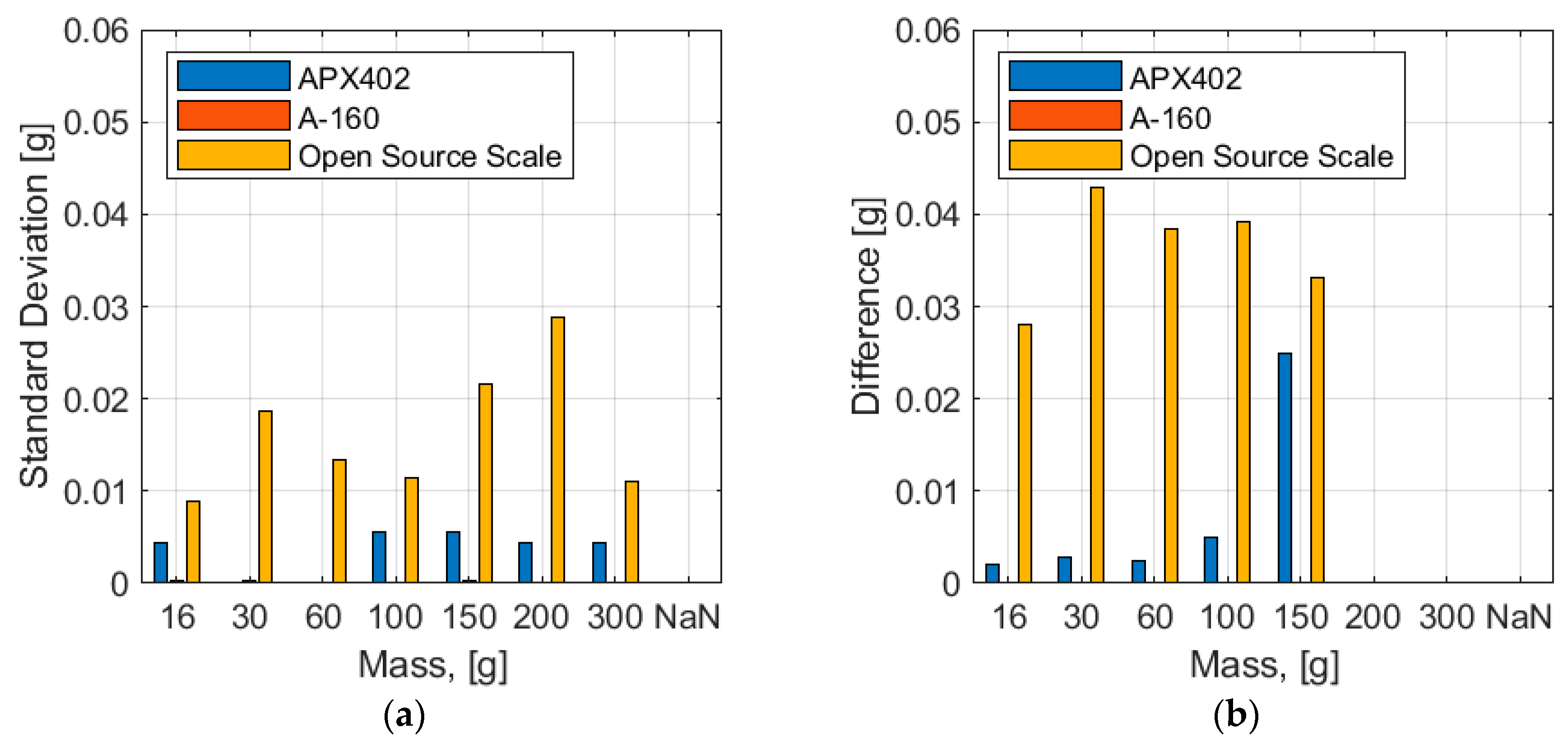
Repeatability testing on the 5kg TAL220 load cell yielded a standard deviation of 0.0163 g on average (max 0.0288 g), as compared to 0.0035 g for the APX402 and 0.0002 g for the A-160. The average absolute difference between the open-source scale and the A-160 was 0.0363 g. The standard deviation and absolute differences are plotted for each discrete mass in Figure 10a,b, respectively.
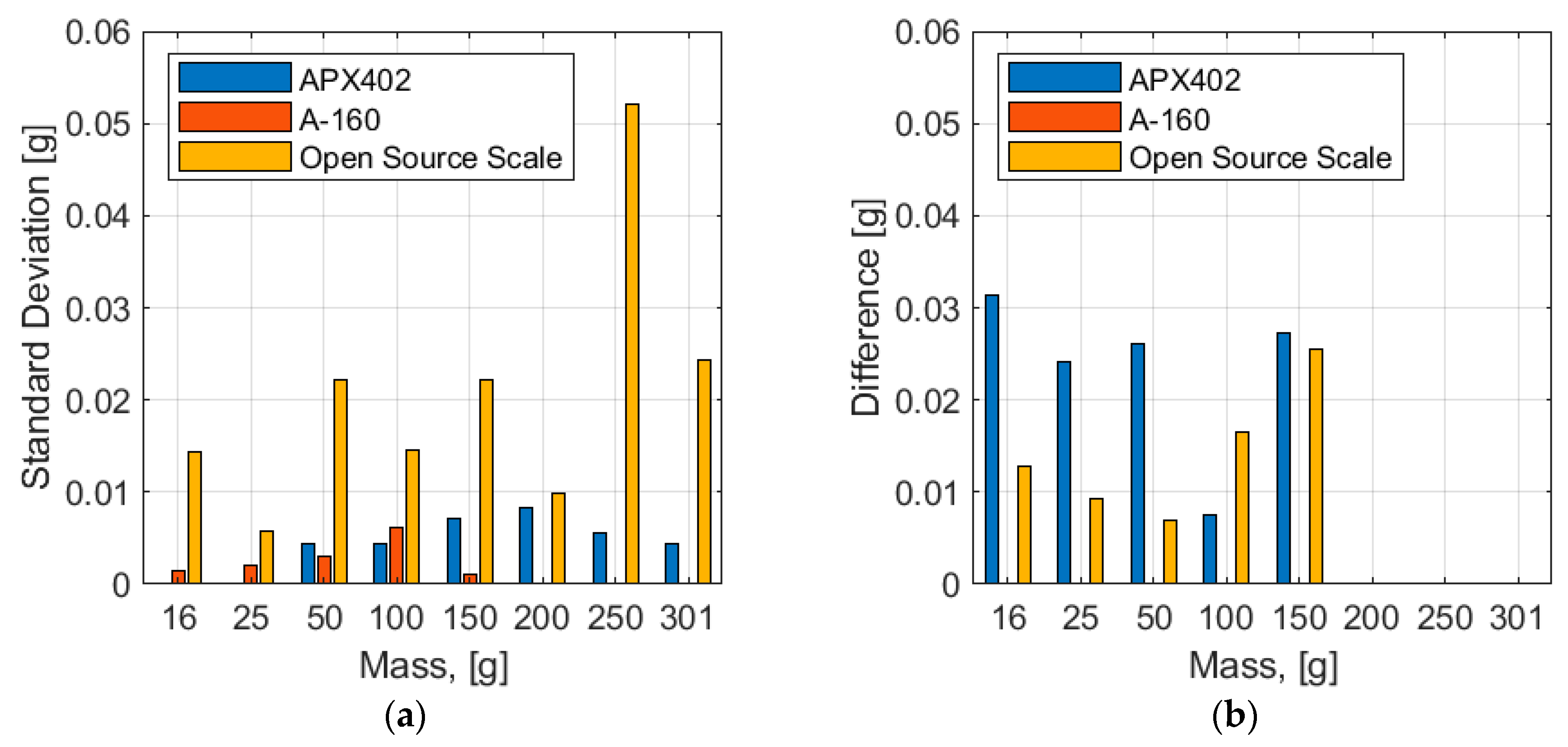
Testing conducted on the 500 g TAL221 load cell yielded a standard deviation of 0.0207 g on average (max 0.0521 g), as compared to 0.0043 g for the APX402 and 0.0027 g for the A-160. The average absolute difference between the open-source scale and the A-160 was 0.0142 g. The standard deviation and absolute differences are plotted for each discrete mass in Figure 11a,b, respectively.
The testing completed on the TAL221 500 g load cell followed the same procedures, but the conditions appear to have been different. The A-160’s standard deviation was an order of magnitude higher than during testing of the TAL220, and the difference between the APX402 and the A-160 was 5 times larger, on average. It is expected that the environment had some effect on testing—it is possible that the ventilation system could have affected measurements by increasing airflow on the scales. It may also be the case that the scales were not properly pre-warmed (powered on for 15 min to an hour) prior to the initiation of testing.
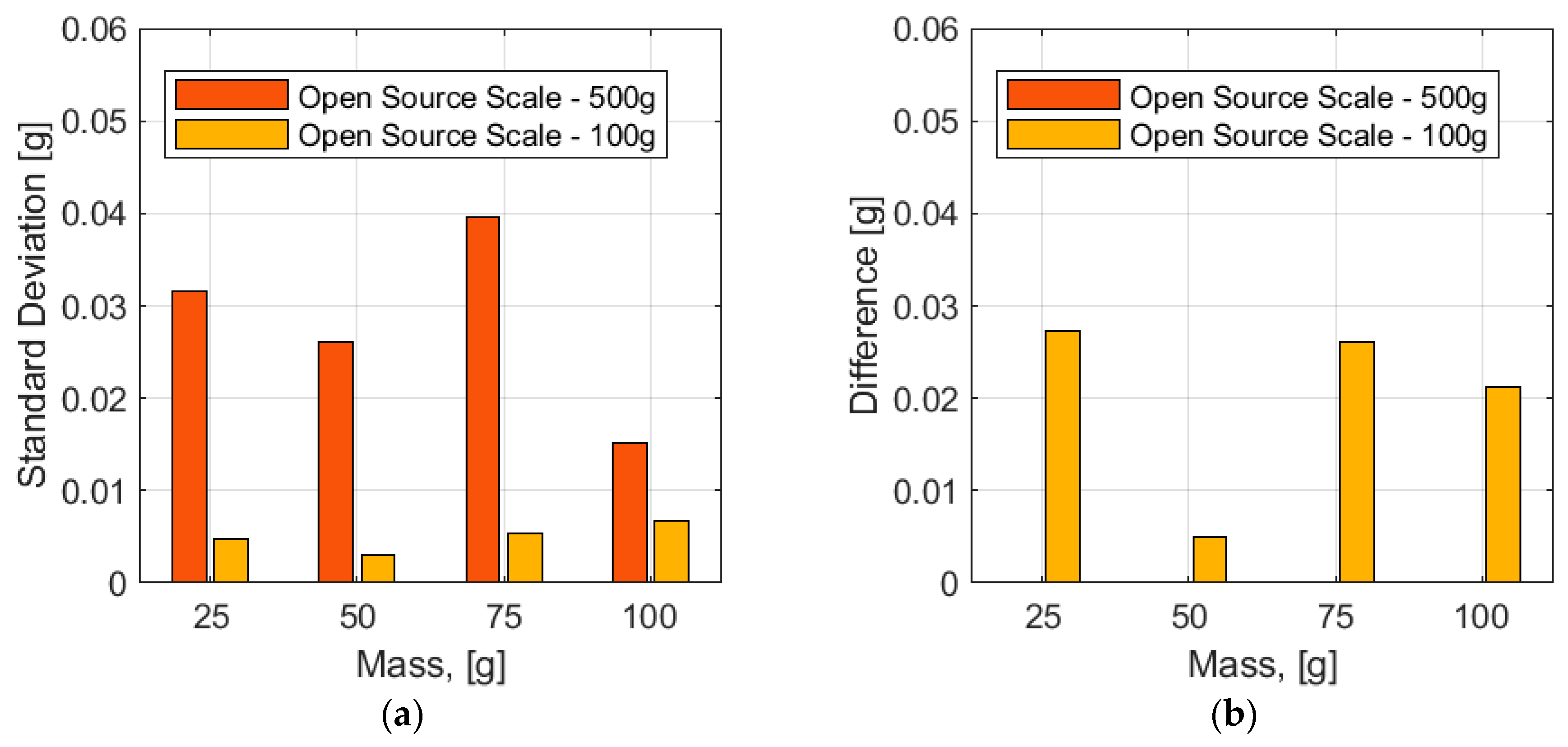
Finally, testing conducted on the 100 g TAL221 yielded a standard deviation of 0.005 g on average (0.0066 g max). This is around 20–50% higher than the standard deviation measured for the APX402 during the two rounds of testing detailed above, indicating the 100 g load cell offers precision on the order of (though slightly lesser than) the APX402. The average difference between the 100 g and 500 g TAL221 load cells was 0.0198 g on average, though the average difference here should not be taken alone to certify the accuracy of the 100 g load cell, as there is unquantified error propagation between the calibration of the 500 g and 100 g load cells. This is the limitation of using the open-source scale to make secondary calibrated masses. The error propagation is a result of the calibration of the 100 g TAL221 against the 500 g TAL221, rather than the A-160. The test results are shown in Figure 12.
These tests showed that the scale tracks linearly with the two lab-grade scales, but its output is less precise. The precision of the scale is a function of the range and style of the load cell. These results support the idea that smaller range load cells produce more precise measurements, with the 100 g TAL221 approaching the precision of the APX402. The average standard deviation () of each load cell tested is compared to its range in Table 3 as a percentage .
The only load cell tested to its full range was the 100 g TAL221 because of its smaller range and the results indicate linear behavior of the load cell across its entire range of measurement.
3.2. Standard Mass Measurements
The testing completed with the standard masses yielded results that vary slightly from those returned during comparison testing. The standard deviation of each dataset entirely represents the variation of the measurement output of the scale, without the influence of repeatability or human error when reading the value from the scale. The 5 kg TAL220 was also tested on two different housings/frames—the 3-D printed PLA housing and a simple wooden frame.
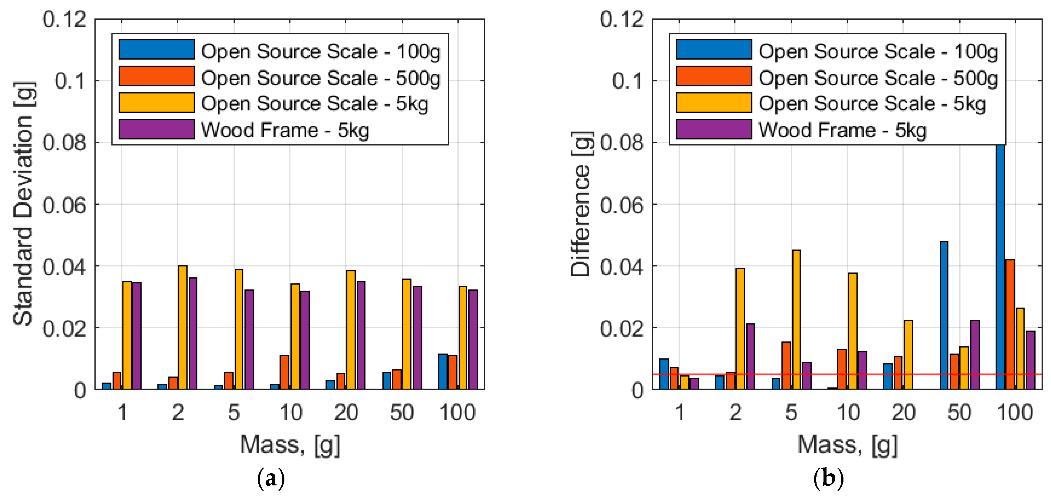
The standard deviations show a similar pattern to the repeatability testing, although both TAL221 load cells performed better in this case than the repeatability testing, while the TAL220 performed slightly worse. The difference in performance may be related to the increased sample size and that the equipment was allowed to warm up prior to testing. These results indicate a direct relationship between load cell range and measurement precision. The standard deviation of each load cell is compared by measurement in Figure 13a and overall in Table 4. Please note that the 100 g TAL221 was out of range when measuring the 100 g standard mass, causing abnormal readout variation and a large error, so that measurement was not included when calculating the average standard deviation shown in Table 4.
Analyzing the difference between the reported mass and the known mass applied to the scale gives an indication of the accuracy of the scale. Zero-offsets (the scale not reading zero when unloaded) were observed in the 5 kg TAL220 measurements. This occurred because the scale was zeroed prior to, but not during testing. To correct for the zero-offset, the average reading of the scale immediately prior to each measurement was subtracted from the average measurement. The resulting (corrected) differences between the reported mass and the actual mass are shown in Figure 13b. This figure also includes a red line indicating the rated accuracy of the weights.
These results indicate that error beyond the accuracy of the weights exist in the scale. This variation may be a result of many factors, including a zero-offset during calibration, temperature variation on the HX711, and, in the case of the 100 g load cell, overloading.
The 5kg TAL220 showed greater variation from the actual mass when installed on the PLA housing when compared to the wooden frame. The behavior is inconsistent and was more pronounced at smaller masses, suggesting that the deformation of the housing is not the cause—although this could very well become an issue with much larger loads. It is possible that the bed of the scale was not seated firmly. Relative motion between the bed and the load cell could change the way the load cell reacts to a load. No significant difference in measurement variation (standard deviation) was observed between the plastic and wooden housings.
3.3. Economic Analysis
The total mass of the 3-D printed components is m = 18.74 g + 33.22 g + 65.44 g = 117.40 g, bringing the cost of printed components to $2.46. Assuming no components are previously owned, the total investment (buying bulk items) for the basic scale is $51.36 ($31.12 if using an Arduino derivative [67]), plus $14.19 to add an LCD, and $4.00 to use a wall outlet for power. Accounting for the value of individual components from within bulk purchases, the cost of the scale is $40.75 ($20.51 with derivative), plus $6.26 for an LCD and $4.00 to use a wall outlet for power. These results are summarized in Table 5. These estimates do not account for taxes or the cost of shipping, jumper wires, or solder.
4. Discussion
4.1. Open-Source Scale for Distributed Manufacturing
The open-source scale showed linearity consistent with data sheet claims during testing. The precision of the load cell is dependent on the type and range of the load cell, meaning that precision requirements should inform decision making during load cell selection. All three load cells tested provide repeatability (one standard deviation) finer than 0.05 g. A major limitation to the scale is that it is susceptible to environmental effects such as temperature. Documentation from Denver Instruments suggests that powering on the scale for 15+ min prior to testing helps stabilize its output by allowing the components to reach a steady-state temperature [90,91]. This was observed during testing, but not specifically tested. Temperature variations on the HX711 were limited by enclosing the amplifier to reduce airflow, and could be further improved by introducing a temperature sensor to make corrections for environmental variations.
A significant advantage of this scale is that its range and precision is interchangeable to meet varying needs. The serial interface offers the possibility to log data and control the scale during testing, allowing partially and fully automated testing. The open-source nature of the scale makes room for improvement and modification where necessary to meet particular needs. Additionally, the modular nature of its design allows for cost savings by removing un-needed components, such as the LCD in the case of automated/computer-based measurement.
The two proprietary, lab-grade scales that were used for comparison testing are out of production. The best estimate for their cost is listings on eBay, which price the APX402 at $75.00 and the A-160 at $425.00 [95,96]. Both lab scales offer RS232 serial interfaces over which the scale can be controlled and interrogated, similar to the open-source scale. This means that a scale of comparable (although still lesser) precision to the APX402 can be constructed for as low as one third of the cost of used eBay purchases. New scales with comparable capability to the open-source scale come at varying costs, depending on their range, precision, and the presence of a serial interface. Some readily available options are compared to the open scale in Table 6. The percent savings achieved by using the open-source scale are calculated and summarized. As can be seen by Table 6, it is possible to purchase a less expensive scale without serial capability (in this case a kitchen scale), but that there are substantial savings using the open-source approach for scales with serial capability. For lab-grade scales the open-source scale saves between 57% and 83% from the commercially available scales.
In addition, to the benefits of greater control, data-logging, customization, and cost the open-source scale has several other advantages. There are often artificial barriers to obtaining scientific equipment in various countries. First, there are often tariffs, duties, “made in {specific country}” restrictions, and taxes added to importation of scientific equipment. These can combine with other factors such as cost to limit research, medical care and educational opportunities (particularly in the developing world), which hampers economic development [104,105,106]. By being able to fabricate a digital scale from low-cost base components, most of which are widely available, scientists, educators, and medical staff can avoid these additional costs and gain access to the tool. Secondly, the most extreme cases, when countries are in desperate need for a wide range of medical/scientific equipment such as currently underway during the COVID-19 pandemic [107], there are even export bans [108] that would limit scientific access to tools. Personal fabrication overcomes such bans. Third, arbitrary definitions of “equipment” rather than “supplies” [109] can limit a scientists’ ability to spend money in the way their research demands. Again, being able to build equipment from supplies offers scientists more flexibility to obtain tools even in the face of administrative restrictions.
4.2. Future Technical Work
Documentation in the A-160 and APX402 manuals suggest that leaving the scale on for 15–60 min prior to testing will aid in the accuracy and repeatability of measurements by allowing the components to warm up to a stable temperature. This was not done during some of the documented testing as for the majority of laboratory work such actions are unnecessary and may not be conducive to real-world use cases. This can, however, be tested in future development by logging mass and tracking room and component temperatures for long periods of time. Other methods for stabilizing the readout to temperature variations should also be explored. SparkFun’s OpenScale microcontroller implements temperature sensing to correct for temperature and this implementation could be quantified [110].
The data-logging/serial interface capability is currently restricted to a scale that is connected to a computer. The scale could be extended to allow automated serial logging using a device such as SparkFun’s OpenLog, which stores serial output to an SD memory card [111]. This, in combination with battery power, would result in a portable logging scale for use in a variety of environments.
Testing should be conducted to determine the viability of this scale for use in long-term mass studies. Observations during the documented testing show that the scale tends to drift significantly when first turned on. This drift appears to be largely related to temperature, but may be related to other factors, such as load cell creep [61], or electrostatic influences from the housing material and surrounding environment. The design could also be tested/modified to work with higher capacity load cells—the plastic housing is very lightweight, meaning it would deform under heavy loads, resulting in side- and angular-loading on the load cell, which can cause error in measurements [61]. High-weight scales can approach $1000 in cost, but this open-source scale could be modified to handle larger weight ranges (e.g., with a higher capacity load cell and more rigid housing) without much cost increase [79,112]. In addition, because the code is freely shared it can be integrated into more complicated systems such as feedback loop additive manufacturing, melt flow index and dynamic off-gassing experiments. In completing further testing, multiple scales should be constructed to test multiple load cells simultaneously, offering more consistent test conditions and results.
5. Conclusions
This study provided designs for a low-cost, easily replicable open-source lab-grade precision digital scale. The designs are released under open-source licenses to enable any lab or individual fabricate it using open-source 3-D printers and widely available low-cost components. Over several versions of the design with different load cells the open-source scale was found to be repeatable within 0.05 g, with even better precision depending on the load cell range and style. The scale tracks linearly with proprietary lab-grade scales, meeting the performance specified in the load cell data sheets, indicating that it is accurate across the range of the load cell installed. The scale can be produced at significant cost savings compared to scales of comparable range and precision when serial capability is present. The cost savings increase significantly as the range of the scale increases. The ability to use the same hardware and firmware for a variety of load cells also makes the scale flexible to time-varying needs in a laboratory setting.
Supplementary Materials
The following are available online at https://www.mdpi.com/2410-390X/4/3/18/s1, Video S1: MOST OS Balance v1.mpeg.
Author Contributions
Conceptualization, B.R.H. and J.M.P.; methodology, B.R.H. and J.M.P.; software, B.R.H.; validation, B.R.H.; formal analysis, B.R.H. and J.M.P.; investigation, B.R.H. and J.M.P.; resources, J.M.P.; data curation, B.R.H.; writing—original draft preparation, B.R.H. and J.M.P.; writing—review and editing, B.R.H. and J.M.P.; visualization, B.R.H.; funding acquisition, J.M.P. All authors have read and agreed to the published version of the manuscript.
Funding
This research was funded by Aleph Objects and the Richard Witte Endowment.
Acknowledgments
The authors would like to thank P. Heiden and A. Patil for technical assistance and use of equipment.
Conflicts of Interest
The authors declare no conflict of interest. The funders had no role in the design of the study; in the collection, analyses, or interpretation of data; in the writing of the manuscript; or in the decision to publish the results.
References
- Fogel, K. Producing Open Source Software: How to Run a Successful Free Software Project; O’Reilly Media Inc.: Sebastopol, CA, USA, 2005; ISBN 978-0-596-55299-2. [Google Scholar]
- Webert, S. The Success of Open Source; Harvard University Press: Cambridge, MA, USA, 2004; ISBN 978-0-674-01292-9. [Google Scholar]
- Gibb, A. Building Open Source Hardware: DIY Manufacturing for Hackers and Makers; Pearson Education: London, UK, 2014. [Google Scholar]
- Ackerman, J.R. Toward open source hardware. U. Dayt. L. Rev. 2008, 34, 183–222. [Google Scholar]
- Pearce, J.M. Building research equipment with free, open-source hardware. Science 2012, 337, 1303–1304. [Google Scholar] [CrossRef]
- Pearce, J. Open-Source Lab: How to Build Your Own Hardware and Reduce Research Costs; Elsevier: New York, NY, USA, 2013. [Google Scholar]
- Da Costa, E.T.; Mora, M.F.; Willis, P.A.; Lago, C.L.; Jiao, H.; Garcia, C.D. Getting started with open-hardware: Development and control of microfluidic devices. Electrophoresis 2014, 35, 2370–2377. [Google Scholar] [CrossRef] [PubMed]
- Von Hippel, E. Democratizing innovation: The evolving phenomenon of user innovation. JFB 2005, 55, 63–78. [Google Scholar] [CrossRef]
- Powell, A. Democratizing production through open source knowledge: From open software to open hardware. Media Cult. Soc. 2012, 34, 691–708. [Google Scholar] [CrossRef] [Green Version]
- Blikstein, P. Digital fabrication and “making” in education: The democratization of invention. FabLabs Mach. Mak. Invent. 2013, 4, 1–21. [Google Scholar]
- Gershenfeld, N. Fab: The Coming Revolution on Your Desktop—From Personal Computers to Personal Fabrication; Basic Books: New York, NY, USA, 2008; ISBN 978-0-7867-2204-4. [Google Scholar]
- Wittbrodt, B.T.; Glover, A.G.; Laureto, J.; Anzalone, G.C.; Oppliger, D.; Irwin, J.L.; Pearce, J.M. Life-cycle economic analysis of distributed manufacturing with open-source 3-D printers. Mechatronics 2013, 23, 713–726. [Google Scholar] [CrossRef] [Green Version]
- King, D.L.; Babasola, A.; Rozario, J.; Pearce, J.M. Mobile Open-Source Solar-Powered 3-D Printers for Distributed Manufacturing in Off-Grid Communities. Chall. Sustain. 2014, 2, 18–27. [Google Scholar] [CrossRef]
- Wittbrodt, B.; Laureto, J.; Tymrak, B.; Pearce, J. Distributed manufacturing with 3-d printing: A case study of recreational vehicle solar photovoltaic mounting systems. J. Frugal Innov. 2015, 1, 1–7. [Google Scholar] [CrossRef] [Green Version]
- Sells, E.; Bailard, S.; Smith, Z.; Bowyer, A.; Olliver, V. RepRap: The replicating rapid prototyper-maximizing customizability by breeding the means of production. In Proceedings of the World Conference on Mass Customization and Personalization, Cambridge, MA, USA, 7–10 October 2007. [Google Scholar]
- Jones, R.; Haufe, P.; Sells, E.; Iravani, P.; Olliver, V.; Palmer, C.; Bowyer, A. RepRap-the replicating rapid prototyper. Robotica 2011, 29, 177–191. [Google Scholar] [CrossRef] [Green Version]
- Bowyer, A. 3D Printing and humanity’s first imperfect replicator. 3D Print. Addit. Manuf. 2014, 1, 4–5. [Google Scholar] [CrossRef]
- Kietzmann, J.; Pitt, L.; Berthon, P. Disruptions, decisions, and destinations: Enter the age of 3-D printing and additive manufacturing. Bus. Horiz. 2015, 58, 209–215. [Google Scholar] [CrossRef]
- Lipson, H.; Kurman, M. Fabricated: The New World of 3D Printing; John Wiley & Sons: Chichester, UK, 2013. [Google Scholar]
- Gwamuri, J.; Wittbrodt, B.; Anzalone, N.; Pearce, J. Reversing the trend of large scale and centralization in manufacturing: The case of distributed manufacturing of customizable 3-d-printable self-adjustable glasses. Chall. Sustain. 2014, 2, 30–40. [Google Scholar] [CrossRef]
- Attaran, M. The rise of 3-D printing: The advantages of additive manufacturing over traditional manufacturing. Bus. Horiz. 2017, 60, 677–688. [Google Scholar] [CrossRef]
- Tanikella, N.G.; Wittbrodt, B.; Pearce, J.M. Tensile strength of commercial polymer materials for fused filament fabrication 3D printing. Addit. Manuf. 2017, 15, 40–47. [Google Scholar] [CrossRef] [Green Version]
- Baden, T.; Chagas, A.M.; Gage, G.; Marzullo, T.; Prieto-Godino, L.L.; Euler, T. Open labware: 3-D printing your own lab equipment. PLoS Biol. 2015, 13, e1002086. [Google Scholar] [CrossRef] [PubMed]
- Coakley, M.; Hurt, D.E. 3D Printing in the laboratory: Maximize time and funds with customized and open-source labware. J. Lab. Autom. 2016, 21, 489–495. [Google Scholar] [CrossRef] [Green Version]
- Zhang, C.; Wijnen, B.; Pearce, J.M. Open-Source 3-D platform for low-cost scientific instrument ecosystem. J. Lab. Autom. 2016, 21, 517–525. [Google Scholar] [CrossRef] [Green Version]
- Dhankani, K.C.; Pearce, J.M. Open source laboratory sample rotator mixer and shaker. HardwareX 2017, 1, 1–12. [Google Scholar] [CrossRef]
- Trivedi, D.K.; Pearce, J.M. Open Source 3-D Printed Nutating Mixer. Appl. Sci. 2017, 7, 942. [Google Scholar] [CrossRef]
- Zhang, C.; Anzalone, N.C.; Faria, R.P.; Pearce, J.M. Open-Source 3D-Printable Optics Equipment. PLoS ONE 2013, 8, e59840. [Google Scholar] [CrossRef] [Green Version]
- Winters, B.J.; Shepler, D. 3D printable optomechanical cage system with enclosure. HardwareX 2018, 3, 62–81. [Google Scholar] [CrossRef]
- Agcayazi, T.; Foster, M.; Kausche, H.; Gordon, M.; Bozkurt, A. Multi-axis stress sensor characterization and testing platform. HardwareX 2019, 5, e00048. [Google Scholar] [CrossRef]
- Delmans, M.; Haseloff, J. µCube: A Framework for 3D Printable Optomechanics; Ubiquity Press: London, UK, 2018. [Google Scholar]
- Sharkey, J.P.; Foo, D.C.W.; Kabla, A.; Baumberg, J.J.; Bowman, R.W. A one-piece 3D printed flexure translation stage for open-source microscopy. Rev. Sci. Instrum. 2016, 87, 025104. [Google Scholar] [CrossRef] [Green Version]
- Collins, J.T.; Knapper, J.; Stirling, J.; Mduda, J.; Mkindi, C.; Mayagaya, V.; Mwakajinga, G.A.; Nyakyi, P.T.; Sanga, V.L.; Carbery, D.; et al. Robotic microscopy for everyone: The OpenFlexure Microscope. bioRxiv 2019, 11, 2447–2460. [Google Scholar] [CrossRef]
- Grant, S.D.; Cairns, G.S.; Wistuba, J.; Patton, B.R. Adapting the 3D-printed Openflexure microscope enables computational super-resolution imaging. F1000Res 2019, 8. [Google Scholar] [CrossRef]
- Anzalone, G.C.; Glover, A.G.; Pearce, J.M. Open-Source Colorimeter. Sensors 2013, 13, 5338–5346. [Google Scholar] [CrossRef] [Green Version]
- Kelley, C.D.; Krolick, A.; Brunner, L.; Burklund, A.; Kahn, D.; Ball, W.P.; Weber-Shirk, M. An Affordable Open-Source Turbidimeter. Sensors 2014, 14, 7142–7155. [Google Scholar] [CrossRef] [Green Version]
- Wijnen, B.; Anzalone, G.C.; Pearce, J.M. Open-source mobile water quality testing platform. J. Water Sanit. Hyg. Dev. 2014, 4, 532–537. [Google Scholar] [CrossRef]
- Wittbrodt, B.T.; Squires, D.A.; Walbeck, J.; Campbell, E.; Campbell, W.H.; Pearce, J.M. Open-Source Photometric System for Enzymatic Nitrate Quantification. PLoS ONE 2015, 10, e0134989. [Google Scholar] [CrossRef]
- Wijnen, B.; Hunt, E.J.; Anzalone, G.C.; Pearce, J.M. Open-Source Syringe Pump Library. PLoS ONE 2014, 9, e107216. [Google Scholar] [CrossRef] [Green Version]
- Bravo-Martinez, J. Open source 3D-printed 1000 μL micropump. HardwareX 2018, 3, 110–116. [Google Scholar] [CrossRef]
- Pusch, K.; Hinton, T.J.; Feinberg, A.W. Large volume syringe pump extruder for desktop 3D printers. HardwareX 2018, 3, 49–61. [Google Scholar] [CrossRef]
- Garcia, V.E.; Liu, J.; DeRisi, J.L. Low-cost touchscreen driven programmable dual syringe pump for life science applications. HardwareX 2018, 4, e00027. [Google Scholar] [CrossRef]
- Klar, V.; Pearce, J.M.; Kärki, P.; Kuosmanen, P. Ystruder: Open source multifunction extruder with sensing and monitoring capabilities. HardwareX 2019, 6, e00080. [Google Scholar] [CrossRef]
- Pearce, J.M.; Anzalone, N.C.; Heldt, C.L. Open-Source Wax RepRap 3-D Printer for Rapid Prototyping Paper-Based Microfluidics. J. Lab. Autom. 2016, 21, 510–516. [Google Scholar] [CrossRef] [Green Version]
- Lake, J.R.; Heyde, K.C.; Ruder, W.C. Low-cost feedback-controlled syringe pressure pumps for microfluidics applications. PLoS ONE 2017, 12. [Google Scholar] [CrossRef]
- Kong, D.S.; Thorsen, T.A.; Babb, J.; Wick, S.T.; Gam, J.J.; Weiss, R.; Carr, P.A. Open-source, community-driven microfluidics with Metafluidics. Nat. Biotechnol. 2017, 35, 523–529. [Google Scholar] [CrossRef]
- Niezen, G.; Eslambolchilar, P.; Thimbleby, H. Open-source hardware for medical devices. BMJ Innov. 2016, 2, 78–83. [Google Scholar] [CrossRef] [Green Version]
- Daniel, K.F.; Peter J, G. Open-Source Hardware Is a Low-Cost Alternative for Scientific Instrumentation and Research. Mod. Instrum. 2012, 2012. [Google Scholar] [CrossRef] [Green Version]
- Pearce, J.M. Laboratory equipment: Cut costs with open-source hardware. Nature 2014, 505. [Google Scholar] [CrossRef] [PubMed] [Green Version]
- Pearce, J.M. Impacts of Open Source Hardware in Science and Engineering. Bridge 2017, 47, 24–31. [Google Scholar]
- Pearce, J. Quantifying the Value of Open Source Hardware Development. Mod. Econ. 2015, 6, 1–11. [Google Scholar] [CrossRef] [Green Version]
- Pearce, J.M. Return on investment for open source scientific hardware development. Sci. Public Policy 2016, 43, 192–195. [Google Scholar] [CrossRef]
- Hietanen, I.; Heikkinen, I.T.S.; Savin, H.; Pearce, J.M. Approaches to open source 3-D printable probe positioners and micromanipulators for probe stations. HardwareX 2018, 4, e00042. [Google Scholar] [CrossRef]
- Dryden, M.D.M.; Fobel, R.; Fobel, C.; Wheeler, A.R. Upon the Shoulders of Giants: Open-Source Hardware and Software in Analytical Chemistry. Anal. Chem. 2017, 89, 4330–4338. [Google Scholar] [CrossRef] [PubMed] [Green Version]
- Quartz Crystal Microbalance with Dissipation Monitoring: The First Scientific QCM Entirely Open Source. Available online: https://openqcm.com/ (accessed on 7 April 2020).
- Politi, J.; Dardano, P.; Caliò, A.; Iodice, M.; Rea, I.; De Stefano, L. Reversible sensing of heavy metal ions using lysine modified oligopeptides on porous silicon and gold. Sens. Actuators B Chem. 2017, 244, 142–150. [Google Scholar] [CrossRef]
- Frijns, E.; Verstraelen, S.; Stoehr, L.C.; Van Laer, J.; Jacobs, A.; Peters, J.; Tirez, K.; Boyles, M.S.P.; Geppert, M.; Madl, P.; et al. A Novel Exposure System Termed NAVETTA for In Vitro Laminar Flow Electrodeposition of Nanoaerosol and Evaluation of Immune Effects in Human Lung Reporter Cells. Environ. Sci. Technol. 2017, 51, 5259–5269. [Google Scholar] [CrossRef] [Green Version]
- Ventura, B.D.; Iannaccone, M.; Funari, R.; Ciamarra, M.P.; Altucci, C.; Capparelli, R.; Roperto, S.; Velotta, R. Effective antibodies immobilization and functionalized nanoparticles in a quartz-crystal microbalance-based immunosensor for the detection of parathion. PLoS ONE 2017, 12, e0171754. [Google Scholar] [CrossRef] [Green Version]
- Fries, M.D.F. The Opera Instrument: An Advanced Curation Development for Mars Sample Return Organic Contamination Monitoring; NASA: Woodlands, TX, USA, 2018.
- Muckley, E.S.; Naguib, M.; Ivanov, I.N. Multi-modal, ultrasensitive, wide-range humidity sensing with Ti3C2 film. Nanoscale 2018, 10, 21689–21695. [Google Scholar] [CrossRef]
- Scale Manufacturers Association Load Cell Application and Test Guideline. Available online: http://www.scalemanufacturers.org/pdf/loadcellapplicationtestguidelineapril2010.pdf (accessed on 13 April 2020).
- Xiamen Ocular 1602 LCD Data Sheet. Available online: https://www.sparkfun.com/datasheets/LCD/GDM1602K.pdf (accessed on 30 March 2020).
- AVIA Semiconductor HX711 Data Sheet. Available online: https://cdn.sparkfun.com/datasheets/Sensors/ForceFlex/hx711_english.pdf (accessed on 30 March 2020).
- Arduino Arduino—Board. Available online: https://www.arduino.cc/en/reference/board (accessed on 30 March 2020).
- Scale Manufacturers Association SMA SCP-0499 Scale Serial Communication Protocol 1999. Available online: http://www.scalemanufacturers.org/PDF/ScaleCommProtocol5199M1.pdf (accessed on 13 April 2020).
- Arduino Nano. Available online: https://store.arduino.cc/usa/arduino-nano (accessed on 6 April 2020).
- Geekcreit Nano V3 Module with USB Cable. Available online: https://www.banggood.com/ATmega328P-Nano-V3-Module-Improved-Version-With-USB-Cable-Development-Board-p-933647.html (accessed on 6 April 2020).
- AmazonBasics USB A-miniB. Available online: https://www.amazon.com/AmazonBasics-USB-2-0-Cable-Male/dp/B00NH13S44 (accessed on 6 April 2020).
- Amazon 5V USB Wall Charger. Available online: https://www.amazon.com/Certified-Charger-FONKEN-universal-Compatible/dp/B07DCR29GN/ref=sr_1_3?crid=2T9NB566GJAS4&dchild=1&keywords=5v+usb+power+supply&qid=1586183620&s=electronics&sprefix=5v+usb+p%2Celectronics%2C213&sr=1-3 (accessed on 6 April 2020).
- Amazon HX711 and TAL220. Available online: https://www.amazon.com/KNACRO-Converter-Breakout-Portable-Electronic/dp/B078W2VCP2/ref=sr_1_1?dchild=1&keywords=tal220&qid=1586183945&sr=8-1&th=1 (accessed on 6 April 2020).
- Industries, Adafruit. Tactile Button Switch (6mm) × 20 Pack. Available online: https://www.adafruit.com/product/367 (accessed on 6 April 2020).
- Industries, Adafruit. Adafruit Full Sized Breadboard. Available online: https://www.adafruit.com/product/239 (accessed on 6 April 2020).
- Banggood 40pcs Double Side Prototype PCB. Available online: https://www.banggood.com/Geekcreit-40pcs-FR-4-2_54mm-Double-Side-Prototype-PCB-Printed-Circuit-Board-p-995732.html (accessed on 6 April 2020).
- Arducam 1602 16 × 2 LCD Display Module. Available online: https://www.amazon.com/Arducam-Display-Controller-Character-Backlight/dp/B019D9TYMI (accessed on 6 April 2020).
- Potentiometers|Mouser. Available online: https://www.mouser.com/Passive-Components/Potentiometers-Trimmers-Rheostats/Potentiometers/_/N-9q0yp?Ns=Pricing|0 (accessed on 14 April 2020).
- Resistor Kit—1/4W (500 total) —COM-10969—SparkFun Electronics. Available online: https://www.sparkfun.com/products/10969 (accessed on 6 April 2020).
- Headers, Adafruit. Available online: https://www.adafruit.com/category/154 (accessed on 6 April 2020).
- HTC-Sensor TAL220 Data Sheet. Available online: https://cdn.sparkfun.com/datasheets/Sensors/ForceFlex/TAL220M4M5Update.pdf (accessed on 4 April 2020).
- HTC-Sensor TAL221 Data Sheet. Available online: https://cdn.sparkfun.com/assets/9/9/a/f/3/TAL221.pdf (accessed on 4 April 2020).
- Mini Load Cell—100 g, Straight Bar (TAL221), SparkFun Electronics. Available online: https://www.sparkfun.com/products/14727 (accessed on 6 April 2020).
- Open Source Laboratory Logging Digital Scale. Available online: https://osf.io/me9a8/ (accessed on 6 April 2020). [CrossRef]
- GNU General Public License Version 3. Available online: https://www.gnu.org/licenses/gpl-3.0.en.html (accessed on 29 March 2019).
- Cura LulzBot Edition. Available online: https://www.lulzbot.com/cura (accessed on 2 April 2019).
- LulzBot LulzBot TAZ 6. Available online: https://www.lulzbot.com/store/printers/lulzbot-taz-6 (accessed on 20 April 2020).
- Fritzing. Available online: http://fritzing.org/ (accessed on 28 March 2020).
- Arduino HelloWorld. Available online: https://www.arduino.cc/en/Tutorial/HelloWorld (accessed on 28 March 2020).
- SparkFun Basic Character LCD Hookup Guide—learn.sparkfun.com. Available online: https://learn.sparkfun.com/tutorials/basic-character-lcd-hookup-guide (accessed on 30 March 2020).
- Bogde HX711. Available online: https://github.com/bogde/HX711 (accessed on 13 April 2020).
- Hans-Christoph Steiner LiquidCrystal; Arduino Libraries. Available online: https://github.com/arduino-libraries/LiquidCrystal (accessed on 13 April 2020).
- Denver Instruments APX-402 Operators Manual. Available online: http://www.denverinstrument.com/denverusa/media/pdf/archive_manuals/Op-Man-Apex-RevC.pdf (accessed on 16 April 2019).
- Denver Instruments A-160 Operators Manual. Available online: http://www.denverinstrument.com/denverusa/media/pdf/archive_manuals/OpMan_A-Series.pdf (accessed on 16 April 2019).
- Sule, S.S.; Petsiuk, A.L.; Pearce, J.M. Open Source Completely 3-D Printable Centrifuge. Instruments 2019, 3, 30. [Google Scholar] [CrossRef] [Green Version]
- EIA. Electric Power Monthly. Available online: https://www.eia.gov/electricity/monthly/epm_table_grapher.php?t=epmt_5_6_a (accessed on 16 April 2019).
- White MH Build Series PLA Filament—2.85mm (1kg). Available online: https://www.matterhackers.com/store/3d-printer-filament/300mm-pla-filament-white-1-kg (accessed on 20 April 2020).
- eBay Denver APX 402 Scale for Sale Online. Available online: https://www.ebay.com/c/669060320 (accessed on 14 April 2020).
- eBay Denver A-160 Digital Scale for Sale Online. Available online: https://www.ebay.com/itm/Denver-Instruments-Company-Digital-Scale-A-160-/161055820362 (accessed on 14 April 2020).
- AMIR Digital Kitchen Scale, 500 g–0.01 g. Available online: https://www.amazon.com/AMIR-Upgraded-500g-0-01g-Stainless-Batteries/dp/B01HCKQG7G (accessed on 22 April 2020).
- Lab Analytical Balance Scale, 500 g × 0.01 g High Precision Electronic Scientific Scale Peeling Weight Digital Kitchen Precision Balance Jewelry Gold Scale with 200 g Weight Self-Correcting Function (US): Industrial & Scientific. Available online: https://www.amazon.com/Analytical-500gx0-01g-Electronic-Scientific-Self-Correcting/dp/B08591CKQT/ (accessed on 23 April 2020).
- Mein LAY Lab Analytical Electronic Balance Scale Laboratory Balance Digital Kitchen Balance Scale Jewelry Gold Scale Precision Balance (0.01/2000 g): Home & Kitchen. Available online: https://www.amazon.com/Mein-LAY-Analytical-Electronic-Laboratory/dp/B07VRCSFBY/ (accessed on 23 April 2020).
- U.S. SOLID 0.001 g 1 mg Analytical Digital Lab Precision Balance Scale 300 g. Available online: https://www.amazon.com/U-S-Analytical-Digital-Precision-Balance/dp/B017ADAA7C/ (accessed on 23 April 2020).
- U.S. Solid 0.001 g 1 mg Digital Analytical Balance w/RS232 Interface. Available online: https://www.amazon.com/U-S-Solid-Analytical-Laboratories-Calibration/dp/B07Y2SXMTC (accessed on 22 April 2020).
- U.S. Solid Precision Lab Scale 1000 g × 0.01 g-High Precision Analytical Balance w/RS232 Interface, Detachable Draft Shield, Calibration Weight, 100-240 VAC. Available online: https://www.amazon.com/U-S-Solid-Precision-Analytical-Detachable/dp/B07YL1B146/?th=1 (accessed on 23 April 2020).
- CGOLDENWALL 5000 g 5 kg 0.01 g Lab Analytical Balance RS232. Available online: https://www.amazon.com/Analytical-Precision-Electronic-Calibration-Commercial/dp/B07DCM3CFC (accessed on 22 April 2020).
- Ross, A.R.; Lewin, K.M. Science Kits in Developing Countries: An Appraisal of Potential; UNESCO: London, UK, 1992; pp. 1–120. [Google Scholar]
- Gwamuri, J.; Pearce, J.M. Open source 3D printers: An appropriate technology for building low cost optics labs for the developing communities. In Proceedings of the 14th Conference on Education and Training in Optics and Photonics: ETOP 2017, Hangzhou, China, 29–31 May 2017; Volume 10452, p. 104522S. [Google Scholar]
- De Maria, C.; Di Pietro, L.; Ravizza, A.; Lantada, A.D.; Ahluwalia, A.D. Chapter 2—Open-source medical devices: Healthcare solutions for low-, middle-, and high-resource settings. In Clinical Engineering Handbook, 2nd ed.; Iadanza, E., Ed.; Academic Press: Cambridge, MA, USA, 2020; pp. 7–14. ISBN 978-0-12-813467-2. [Google Scholar]
- Pearce, J. Distributed Manufacturing of Open-Source Medical Hardware for Pandemics. Preprints 2020, 4, 49. [Google Scholar] [CrossRef]
- Sebastian, C.; di Donato, V.; CNN. In the Race to Secure Medical Supplies, Countries Ban or Restrict Exports. Available online: https://www.cnn.com/2020/03/27/business/medical-supplies-export-ban/index.html (accessed on 15 April 2020).
- Pearce, J.M. Undermined by overhead accounting. Science 2016, 352, 158–159. [Google Scholar] [CrossRef] [PubMed]
- SparkFun OpenScale Applications and Hookup Guide—SparkFun. Available online: https://learn.sparkfun.com/tutorials/openscale-applications-and-hookup-guide#calibration-suggestions (accessed on 16 March 2020).
- SparkFun OpenLog—DEV-13712. Available online: https://www.sparkfun.com/products/13712 (accessed on 14 April 2020).
- GMM Technoworld 50 kg/1 g 2 kg/0.05 g Digital Counting Scale with Dual Platter & PC Connection. Available online: https://testmeter.sg/webshaper/store/viewprod.asp?pkproductitem=432&pkproduct= (accessed on 22 April 2020).
Figure 1.
Electrical circuit breadboard layout. Please note that all components connected to and including the LCD are optional.
Figure 1.
Electrical circuit breadboard layout. Please note that all components connected to and including the LCD are optional.

Figure 2.
Electrical circuit wiring diagram. Pinouts on the Arduino were selected to reduce the number of required jumper wires when using an Arduino Nano. Pinout selection can be modified in the firmware header file, Pinouts.hpp. Changing micro-controllers or pinouts may change the header pin requirements relative to the listing in Table 1.

Figure 3.
The circuit was assembled on a solder circuit board using jumper wires and header pins. The female header pins connect to the Arduino Nano and the HX711. The male header pins connect to the load cell and the LCD. The tare push-button is attached via twisted pair to allow installation on the face of the scale. (a) The soldered components were arranged in such a way to minimize wire use and to properly place the Arduino when installed in the base. (b) Shows the final circuit board.

Figure 4.
Key features of the base include standoffs to mount the load cell, locators for the screen and circuit board, and a slot for access to the Arduino Nano’s USB port. The base also has a snap-seam to attach the cover to the base, enclosing the internal components.
Figure 4.
Key features of the base include standoffs to mount the load cell, locators for the screen and circuit board, and a slot for access to the Arduino Nano’s USB port. The base also has a snap-seam to attach the cover to the base, enclosing the internal components.

Figure 5.
The circuit board fits into the bosses on the right side of the base to hold it in place. The twisted pair was fed through the hole for the push-button and a set of female–male jumper wires were connected to the load cell header pins to reach the TAL221 wires.
Figure 5.
The circuit board fits into the bosses on the right side of the base to hold it in place. The twisted pair was fed through the hole for the push-button and a set of female–male jumper wires were connected to the load cell header pins to reach the TAL221 wires.

Figure 6.
The LCD is held in place by two locators behind the slot for the screen. Its wires are tucked under a plastic wire manager attached to the TAL220 boss, then connected to the circuit board.
Figure 6.
The LCD is held in place by two locators behind the slot for the screen. Its wires are tucked under a plastic wire manager attached to the TAL220 boss, then connected to the circuit board.

Figure 7.
(a) The TAL221 load cell should be installed with the wires leading off the end of the load cell attached to the base—the M5 tapped holes. Please note that the button is also installed. (b) After snapping on the lid, the bed can be attached to the free end of the load cell using two M4 bolts.

Figure 8.
(a) The cover must be sandwiched between the load cell and the bed prior to attaching to the base. Note the direction the load cell is aimed so it will rest on the TAL221 boss when the cover is snapped on. (b) After connecting the load cell to the controller, the cover is snapped on and the TAL221 is screwed to the base using two M3 bolts. This must be done by feel, but does not take very long.

Figure 9.
The scale returns a readout similar to the one shown during initialization. The readout indicates the action in progress, success, and returns the sensitivity value when reading from memory.
Figure 9.
The scale returns a readout similar to the one shown during initialization. The readout indicates the action in progress, success, and returns the sensitivity value when reading from memory.

Figure 10.
The 5kg load cell results are shown (a) The standard deviation (sample of 5 measurements) averaged to 0.0163 g. This is large relative to the APX402 and the A-160; (b) The absolute value of the difference between each scale and the A-160 is shown. The open-source scale averaged a difference of 0.0363 g.

Figure 11.
The 500 g load cell test results are shown. (a) The standard deviation (sample of 5 measurements) averaged to 0.0207 g for the open-source scale. This is large relative to the lab-grade scales; (b) The absolute value of the difference between the average measurements by the A-160 and the other two scales are shown. The open-source scale average measurement was within 0.0142 g of the A-160, on average.

Figure 12.
The 100 g load cell test results are shown. (a) The standard deviation (sample of 5 measurements) averaged to 0.005 g for the open-source scale. This is close to that of the lab-grade scales (on the same order as the APX402); (b) The absolute value of the difference between the average measurements by the 500 g TAL221 and the other two scales are shown. The 100 g TAL221 average measurement was within 0.0198 g of the 500 g TAL221, on average.

Figure 13.
The standard mass test results are shown. (a) The standard deviation (sample of at least 48 measurements) increased with the range of the load cell; there is little difference between the PLA housing and wood frame. (b) The absolute value of the difference between the average measurements of each scale and the nominal mass of the weights is shown. The accuracy range for the weights is indicated by a red line.


Table 1.
Visual bill of materials separated by mechanical and electrical components.
| Component | Photograph | |
|---|---|---|
| 3-D Printed Components | ||
| Base Print in normal orientation. Can be printed without supports. |  | |
| Cover Print in either orientation. Can be printed without support, but this sacrifices top finish. |  |  |
| Bed Print in either orientation. Can be printed without support, but this sacrifices top finish. |  |  |
| Cover (Optional) Print upside-down without supports. This is used to reduce air currents for higher accuracy and precision. |  |  |
| Electronic Components | ||
| Arduino Microcontroller (Nano) $20.70 [66] (Derivative available with cable for $5.72 [67]) |  | |
| USB-A to mini-B USB (or micro, or USB-B, depending on the specific Arduino in use) $5.26 [68] |  | |
| 5V USB Power Block (Optional) $4.00 [69] |  | |
| HX711 Load cell Amplifier $8.50 with TAL220 [70] |  | |
| Push-Button (Normally Open, Momentary) $2.50 for 20 pack [71] |  | |
| Jumper Wires |  | |
| Breadboard: Option 1: Solderless Breadboard (remains external to scale) $5.95 [72] Option 2: Solder Breadboard (40 × 60 mm), Solder, Soldering Iron $5.99 in 40-pack [73] |  | |
| LCD is optional. The three components below are required if using an LCD. | ||
| 16 × 2 LCD Display $5.99 [74] |  | |
| 10 kΩ Potentiometer $0.25 [75] |  | |
| 220 Ω Resistor $7.95 in 500 pack [76] |  | |
| If using a solderless breadboard, no more electronic components needed. Using a solder breadboard: | ||
| Female Header Pins: 1 × 4 (2) 1 × 8 (1) 1 × 9 (1) $0.95 [77] |  | |
| Male Header Pins: 1 × 12 (1) 1 × 4 (1) $3.00 for 5 × 16 [77] |  | |
| Configuration Specific Hardware | ||
| TAL 220 Load cell configuration | ||
| TAL 220 Load cell (Available in 3, 5, 10, 20, 25, 30, 50, 80, 100, 120, 200 kg ranges [78]) Wires terminated in Female 4-pin molex connector with color order: (Red-Black-White-Green) $0.00 with HX711 [70] |  | |
| Fasteners: M4 × 25 mm cap screw (2)—3 mm Allen Key M5 × 25 mm cap screw (2)—4 mm Allen Key <$2.00 from a hardware store |  | |
| TAL 221 Load cell configuration | ||
| TAL 221 Load cell (Available in 100, 150, 200, 300, 500, 750, 1000, and 1500 g ranges [79]) Wires terminated in Female 4-pin molex connector with color order: (Red-Black-White-Green) $8.95 [80] |  | |
| Fasteners: M3 × 20 mm cap screw (4)—2.5 mm Allen Key M3 nut (2)—5.5 mm Socket <$2.00 from a hardware store |  | |
Table 2.
Print Settings.
| Property | PLA | PETG |
|---|---|---|
| Layer Height | 0.14 mm | 0.18 mm |
| Wall Thickness | 2 mm | 1 mm |
| Top/Bottom Thickness | 2 mm | 1 mm |
| Infill | Cubic, 20% | N/A |
| Support Material | Zigzag, Touching Bedplate Only, 30%, 50 degrees | N/A |
| Bed Adhesion | Skirt | Skirt |
| Nozzle Temperature | 205 °C | 230 °C |
| Print Speed | Infill: 40 mm/s, Wall: 30 mm/s, Support: 60 mm/s | Wall: 20 mm/s |
Table 3.
The average standard deviation for each load cell during repeatability testing is compared as a percentage of the load cell’s total range. These results suggest that the precision of the load cell is a function of its range and style.
Table 3.
The average standard deviation for each load cell during repeatability testing is compared as a percentage of the load cell’s total range. These results suggest that the precision of the load cell is a function of its range and style.
| Style/Range | σ | %FS |
|---|---|---|
| TAL220/5000 g | 0.0163 | 0.0004% |
| TAL221/500 g | 0.0207 | 0.0041% |
| TAL221/100 g | 0.0050 | 0.0050% |
Table 4.
The average standard deviation for each load cell during testing with standard masses is compared as a percentage of the load cell’s total range. These results reinforce the idea that the precision of the load cell is a function of its range and style.
Table 4.
The average standard deviation for each load cell during testing with standard masses is compared as a percentage of the load cell’s total range. These results reinforce the idea that the precision of the load cell is a function of its range and style.
| Style/Range | σ | %FS |
|---|---|---|
| TAL220/5000 g | 0.0365 | 0.0007% |
| TAL221/500 g | 0.0071 | 0.0014% |
| TAL221/100 g | 0.0026 | 0.0026% |
Table 5.
The cost of the scale varies based on configuration and initial investment. Using a wall outlet for power (as opposed to a computer) costs an extra $4.00.
Table 5.
The cost of the scale varies based on configuration and initial investment. Using a wall outlet for power (as opposed to a computer) costs an extra $4.00.
| Configuration | Total Investment | Cost Corrected for Bulk Purchases |
|---|---|---|
| No LCD | $51.36/$31.12 1 | $40.75/$20.51 |
| LCD | $65.55/$45.31 | $47.01/$26.77 |
1 Second value uses Arduino derivative.
Table 6.
Several proprietary scales listed online were compared in price and capability to the open-source scale. This was done to indicate the cost savings allowed by the open-source scale, which vary greatly depending on the functionality and range desired.
Table 6.
Several proprietary scales listed online were compared in price and capability to the open-source scale. This was done to indicate the cost savings allowed by the open-source scale, which vary greatly depending on the functionality and range desired.
| Range/Repeatability | Serial Capability | Retail Cost | Percent Savings of Open-Source Scale ($47.01) |
|---|---|---|---|
| 500 g/0.01 g [97] | No | $15 | NA |
| 500 g/0.1 g [98] | No | $88 | −47% |
| 5000 g/0.1 g [99] | No | $55 | −15% |
| 300 g/0.001 g [100] | Yes | $253 | −81% |
| 500 g/0.002 g [101] | Yes | $115 | −59% |
| 600 g/0.01 g [102] | Yes | $110 | −57% |
| 5000 g/0.08 g [103] | Yes | $289 | −83% |
© 2020 by the authors. Licensee MDPI, Basel, Switzerland. This article is an open access article distributed under the terms and conditions of the Creative Commons Attribution (CC BY) license (http://creativecommons.org/licenses/by/4.0/).
Share and Cite
MDPI and ACS Style
Hubbard, B.R.; Pearce, J.M. Open-Source Digitally Replicable Lab-Grade Scales. Instruments 2020, 4, 18. https://doi.org/10.3390/instruments4030018
AMA Style
Hubbard BR, Pearce JM. Open-Source Digitally Replicable Lab-Grade Scales. Instruments. 2020; 4(3):18. https://doi.org/10.3390/instruments4030018
Chicago/Turabian StyleHubbard, Benjamin R., and Joshua M. Pearce. 2020. "Open-Source Digitally Replicable Lab-Grade Scales" Instruments 4, no. 3: 18. https://doi.org/10.3390/instruments4030018