
First Results from the Thomson Scattering Diagnostic on the Large Plasma Device
 ,
,  , , , , and
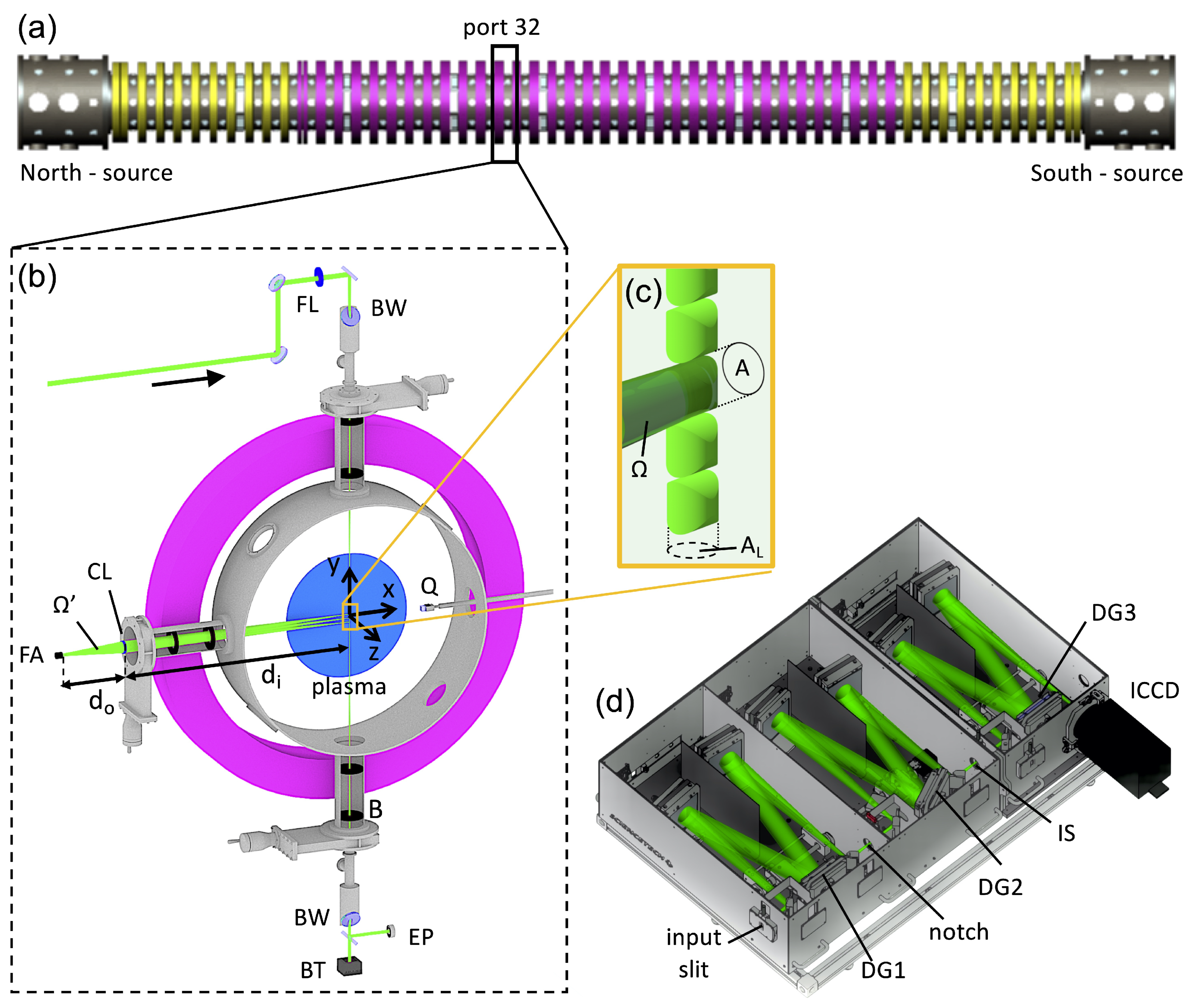
Abstract
:1. Introduction
2. Experimental Setup
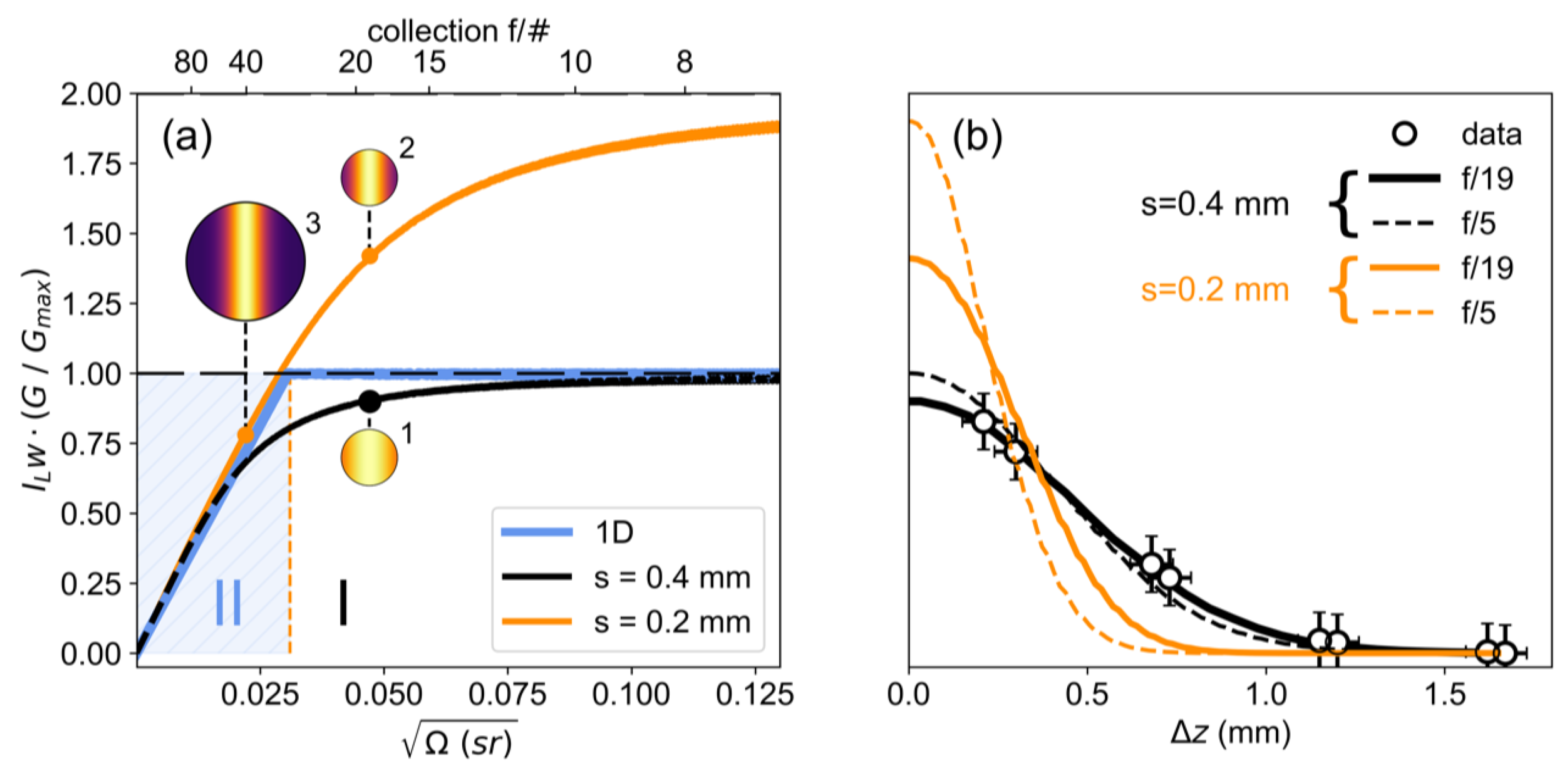
3. Design Considerations
4. Results and Discussion
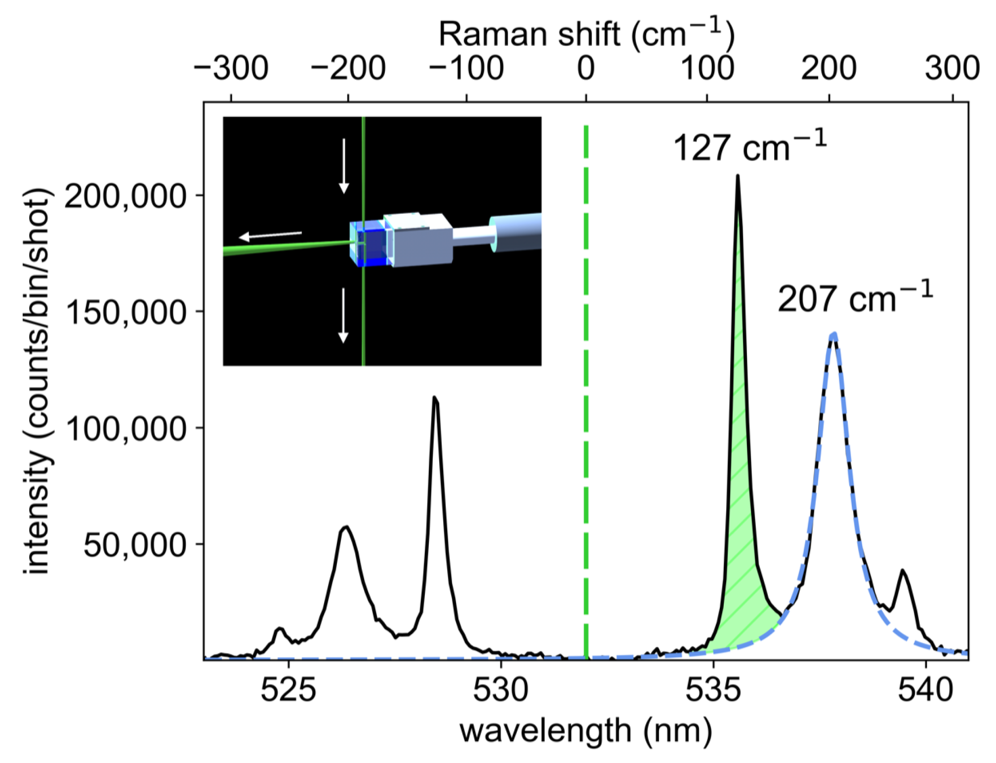
4.1. Absolute Irradiance Calibration
4.2. Thomson Scattering Measurements
4.3. Comparison with Langmuir Probe Measurements
5. Conclusions
Author Contributions
Funding
Institutional Review Board Statement
Informed Consent Statement
Data Availability Statement
Acknowledgments
Conflicts of Interest
References
- Gekelman, W.; Pribyl, P.; Lucky, Z.; Drandell, M.; Leeneman, D.; Maggs, J.; Vincena, S.; Compernolle, B.V.; Tripathi, S.; Morales, G.; et al. The upgraded Large Plasma Device, a machine for studying frontier basic plasma physics. Rev. Sci. Instrum. 2016, 87, 025105. [Google Scholar] [CrossRef] [PubMed] [Green Version]
- Froula, D.; Glenzer, S.; Luhmann, N.C., Jr.; Sheffield, J. Plasma Scattering of Electromagnetic Radiation: Theory and Measurement Techniques. Fusion Sci. Technol. 2012, 61, 104–105. [Google Scholar] [CrossRef]
- Evans, D.; Katzenstein, J. Laser light scattering in laboratory plasmas. Rep. Prog. Phys. 1969, 32, 207–271. [Google Scholar] [CrossRef]
- Chen, F. Lecture Notes on Langmuir Probe Diagnostics; IEEE-ICOPS Meeting: Jeju, Korea, 2003. [Google Scholar]
- Gilmore, M.; Gekelman, W.; Reiling, K.; Peebles, W. A reliable millimeter-wave quadrature interferometer. arXiv 2020, arXiv:2002.11190. [Google Scholar]
- Boivin, R.F.; Kline, J.L.; Scime, E.E. Electron temperature measurement by a helium line intensity ratio method in helicon plasmas. Phys. Plasmas 2001, 8, 5303–5314. [Google Scholar] [CrossRef] [Green Version]
- Bondarenko, A.S.; Schaeffer, D.B.; Everson, E.T.; Clark, S.E.; Constantin, C.G.; Niemann, C. Spectroscopic measurement of high-frequency electric fields in the interaction of explosive debris plasma with magnetized background plasma. Phys. Plasmas 2014, 21, 122112. [Google Scholar] [CrossRef] [Green Version]
- Niemann, C.; Gekelman, W.; Constantin, C.G.; Everson, E.T.; Schaeffer, D.B.; Bondarenko, A.S.; Clark, S.E.; Winske, D.; Vincena, S.; Van Compernolle, B.; et al. Observation of collisionless shocks in a large current-free laboratory plasma. Geophys. Res. Lett. 2014, 41, 7413–7418. [Google Scholar] [CrossRef]
- Schaeffer, D.B.; Winske, D.; Larson, D.J.; Cowee, M.M.; Constantin, C.G.; Bondarenko, A.S.; Clark, S.E.; Niemann, C. On the generation of magnetized collisionless shocks in the large plasma device. Phys. Plasmas 2017, 24, 041405. [Google Scholar] [CrossRef]
- Schaeffer, D.; Cruz, F.; Dorst, R.; Cruz, F.; Heuer, P.; Constantin, C.; Pribyl, P.; Niemann, C.; Silva, L.; Bhattacharjee, A. Laser-Driven, Ion-Sale Magnetospheres in Laboratory Plasmas. I. Experimental Platform and First Results. arXiv 2022, arXiv:2201.02176. [Google Scholar]
- Heuer, P.; Weidl, M.; Dorst, R.; Schaeffer, D.; Tripathi, S.; Vincena, S.; Constantin, C.; Niemann, C.; Wilson, L.B., III; Winske, D. Laboratory Observations of Ultra-low-frequency Analog Waves Driven by the Right-hand Resonant Ion Beam Instability. Astrophys. J. 2020, 891, L11. [Google Scholar] [CrossRef]
- Keenan, B.D.; Le, A.; Winske, D.; Stanier, A.; Wetherton, B.; Cowee, M.; Guo, F. Hybrid particle-in-cell simulations of electromagnetic coupling and waves from streaming burst debris. Phys. Plasmas 2022, 29, 012107. [Google Scholar] [CrossRef]
- Collette, A.; Gekelman, W. Structure of an Exploding Laser-Produced Plasma. Phys. Rev. Lett. 2010, 105, 195003. [Google Scholar] [CrossRef] [PubMed]
- Niemann, C.; Gekelman, W.; Constantin, C.G.; Everson, E.T.; Schaeffer, D.B.; Clark, S.E.; Winske, D.; Zylstra, A.B.; Pribyl, P.; Tripathi, S.K.P.; et al. Dynamics of exploding plasmas in a large magnetized plasma. Phys. Plasmas 2013, 20, 012108. [Google Scholar] [CrossRef] [Green Version]
- Gekelman, W.; Collette, A.; Vincena, S. Three-dimensional current systems generated by plasmas colliding in a background magnetoplasma. Phys. Plasmas 2007, 14, 062109. [Google Scholar] [CrossRef] [Green Version]
- Pilgram, J.; Adams, M.; Constantin, C.; Heuer, P.; Ghazaryan, S.; Kaloyan, M.; Dorst, R.; Schaeffer, D.; Tzeferacos, P.; Niemann, C. High Repetition Rate Exploration of the Biermann Battery Effect in Laser Produced Plasmas over Large Spatial Regions. High Power Laser Sci. Eng. 2022, 2, 1–11. [Google Scholar] [CrossRef]
- Muraoka, K.; Uchino, K.; Bowden, M.D. Diagnostics of low-density glow discharge plasmas using Thomson scattering. Plasma Phys. Control. Fusion 1998, 40, 1221–1239. [Google Scholar] [CrossRef]
- Kono, A.; Nakatani, K. Efficient multichannel Thomson scattering measurement system for diagnostics of low-temperature plasmas. Rev. Sci. Instrum. 2000, 71, 2716–2721. [Google Scholar] [CrossRef]
- Van de Sande, M.J.; Van der Mullen, J.J.A.M. Thomson scattering on a low-pressure, inductively-coupled gas discharge lamp. J. Phys. Appl. Phys. 2002, 35, 1381–1391. [Google Scholar] [CrossRef]
- Belostotskiy, S.G.; Khandelwal, R.; Wang, Q.; Donnelly, V.M.; Economou, D.J.; Sadeghi, N. Measurement of electron temperature and density in an argon microdischarge by laser Thomson scattering. Appl. Phys. Lett. 2008, 92, 221507. [Google Scholar] [CrossRef] [Green Version]
- Yamamoto, N.; Tomita, K.; Sugita, K.; Kurita, T.; Nakashima, H.; Uchino, K. Measurement of xenon plasma properties in an ion thruster using laser Thomson scattering technique. Rev. Sci. Instrum. 2012, 83, 073106. [Google Scholar] [CrossRef]
- Lee, K.Y.; Lee, K.I.; Kim, J.H.; Lho, T. High resolution Thomson scattering system for steady-state linear plasma sources. Rev. Sci. Instrum. 2018, 89, 013508. [Google Scholar] [CrossRef] [PubMed]
- Seo, B.; Bellan, P.M. Experimental investigation of the compression and heating of an MHD-driven jet impacting a target cloud. Phys. Plasmas 2018, 25, 112703. [Google Scholar] [CrossRef]
- Zhao, Y.; Wang, Y.; Shi, J.; Wu, D.; Feng, C.; Wu, G.; Yuan, K.; Ding, H. Comparison of Terahertz time domain spectroscopy and laser Thomson scattering for electron density measurements in inductively coupled plasma discharges. J. Instrum. 2019, 14, C12019. [Google Scholar] [CrossRef]
- Vincent, B.; Tsikata, S.; Mazouffre, S.; Minea, T.; Fils, J. A compact new incoherent Thomson scattering diagnostic for low-temperature plasma studies. Plasma Sources Sci. Technol. 2018, 27, 055002. [Google Scholar] [CrossRef]
- Shi, P.; Srivastav, P.; Beatty, C.; Nirwan, R.S.; Scime, E.E. Incoherent Thomson scattering system for PHAse space MApping (PHASMA) experiment. Rev. Sci. Instrum. 2021, 92, 033102. [Google Scholar] [CrossRef]
- Zweben, S.J.; Caird, J.; Davis, W.; Johnson, D.W.; Le Blanc, B.P. Plasma turbulence imaging using high-power laser Thomson scattering. Rev. Sci. Instrum. 2001, 72, 1151–1154. [Google Scholar] [CrossRef] [Green Version]
- Niemann, C.; Constantin, C.; Schaeffer, D.; Tauschwitz, A.; Weiland, T.; Lucky, Z.; Gekelman, W.; Everson, E.; Winske, D. High-energy Nd:glass laser facility for collisionless laboratory astrophysics. J. Instrum. 2012, 7, P03010. [Google Scholar] [CrossRef]
- Schaeffer, D.; Constantin, C.; Bondarenko, A.; Everson, E.; Niemann, C. Spatially resolved Thomson scattering measurements of the transition from the collective to the non-collective regime in a laser-produced plasma. Rev. Sci. Instrum. 2016, 87, 11E701. [Google Scholar] [CrossRef]
- Ghazaryan, S.; Kaloyan, M.; Niemann, C. Silica Raman scattering probe for absolute calibration of Thomson scattering spectrometers. J. Instrum. 2021, 16, P08045. [Google Scholar] [CrossRef]
- Kaloyan, M.; Ghazaryan, S.; Constantin, C.G.; Dorst, R.S.; Heuer, P.V.; Pilgram, J.J.; Schaeffer, D.B.; Niemann, C. Raster Thomson scattering in large-scale laser plasmas produced at high repetition rate. Rev. Sci. Instrum. 2021, 92, 093102. [Google Scholar] [CrossRef]
- Van de Sande, M. Laser Scattering on Low Temperature Plasmas: HIGH Resolution and Stray Light Rejection. Ph.D. Thesis, Technical University Eindhoven, Eindhoven, The Netherlands, 2002. [Google Scholar] [CrossRef]
- Schaeffer, D.B.; Kugland, N.L.; Constantin, C.G.; Everson, E.; Compernolle, B.V.; Ebbers, C.; Glenzer, S.; Niemann, C. A scalable multipass laser cavity based on injection by frequency conversion for noncollective Thomson scattering. Rev. Sci. Instrum. 2010, 81, 10D518. [Google Scholar] [CrossRef] [PubMed] [Green Version]
- Berni, L.; Campos, D.; Machida, M.; Moshkalyov, S.; Lebedev, S. Molecular Rayleigh scattering as calibration method for Thomson scattering experiments. Braz. J. Phys. 1996, 26, 755. [Google Scholar]
- Flora, F.; Giudicotti, L. Complete calibration of a Thomson scattering spectrometer system by rotational Raman scattering in H2. Appl. Opt. 1987, 26, 4001. [Google Scholar] [CrossRef] [PubMed]
- Ridl, M.J. Optical Design Fundamentals for Infrared Systems, 2nd ed.; SPIE Tutorial Texts in Optical Engineering: Bellingham, WA, USA, 2001; ISBN-13: 978-0819440518. [Google Scholar] [CrossRef]
- Said, A.; Xia, T.; Dogariu, A.; Hagan, D.; Soileau, M.; Stryland, E.V.; Mohebi, M. Measurement of the optical damage threshold in fused quartz. Appl. Opt. 1995, 34, 3374. [Google Scholar] [CrossRef] [Green Version]
- Irisawa, J.; John, P.K. Comparison of Langmuir Double Probe and Laser Scattering Measurements of Plasma Parameters. Rev. Sci. Instrum. 1973, 44, 1021–1023. [Google Scholar] [CrossRef]
- Jones, L.A. Comparison of Langmuir probe and Thomson scattering measurements of electron temperature and density. J. Appl. Phys. 1974, 45, 5206–5208. [Google Scholar] [CrossRef]
- Godyak, V.A.; Alexandrovich, B.M. Comparative analyses of plasma probe diagnostics techniques. J. Appl. Phys. 2015, 118, 233302. [Google Scholar] [CrossRef]
- Ryan, P.J.; Bradley, J.W.; Bowden, M.D. Comparison of Langmuir probe and laser Thomson scattering for electron property measurements in magnetron discharges. Phys. Plasmas 2019, 26, 073515. [Google Scholar] [CrossRef]
- Mott-Smith, H.M.; Langmuir, I. The Theory of Collectors in Gaseous Discharges. Phys. Rev. 1926, 28, 727–763. [Google Scholar] [CrossRef]
- Chen, F.F.; Etievant, C.; Mosher, D. Measurement of Low Plasma Densities in a Magnetic Field. Phys. Fluids 1968, 11, 811–821. [Google Scholar] [CrossRef]


Publisher’s Note: MDPI stays neutral with regard to jurisdictional claims in published maps and institutional affiliations. |
© 2022 by the authors. Licensee MDPI, Basel, Switzerland. This article is an open access article distributed under the terms and conditions of the Creative Commons Attribution (CC BY) license (https://creativecommons.org/licenses/by/4.0/).
Share and Cite
Kaloyan, M.; Ghazaryan, S.; Tripathi, S.P.; Gekelman, W.; Valle, M.J.; Seo, B.; Niemann, C. First Results from the Thomson Scattering Diagnostic on the Large Plasma Device. Instruments 2022, 6, 17. https://doi.org/10.3390/instruments6020017
Kaloyan M, Ghazaryan S, Tripathi SP, Gekelman W, Valle MJ, Seo B, Niemann C. First Results from the Thomson Scattering Diagnostic on the Large Plasma Device. Instruments. 2022; 6(2):17. https://doi.org/10.3390/instruments6020017
Chicago/Turabian StyleKaloyan, Marietta, Sofiya Ghazaryan, Shreekrishna P. Tripathi, Walter Gekelman, Mychal J. Valle, Byonghoon Seo, and Christoph Niemann. 2022. "First Results from the Thomson Scattering Diagnostic on the Large Plasma Device" Instruments 6, no. 2: 17. https://doi.org/10.3390/instruments6020017