Energy Storage Scheduling with an Advanced Battery Model: A Game–Theoretic Approach


School of Computer Science and Mathematics, Kingston University London, Penrhyn Road, Kingston upon Thames KT1 2EE, UK
*
Author to whom correspondence should be addressed.
Inventions 2017, 2(4), 30; https://doi.org/10.3390/inventions2040030
Submission received: 12 September 2017
/
Revised: 25 October 2017
/
Accepted: 13 November 2017
/
Published: 16 November 2017
(This article belongs to the Section Inventions and Innovation in Electrical Engineering/Energy/Communications)
Abstract
:Energy storage systems will play a key role for individual users in the future smart grid. They serve two purposes: (i) handling the intermittent nature of renewable energy resources for a more reliable and efficient system; and (ii) preventing the impact of blackouts on users and allowing for more independence from the grid, while saving money through load-shifting. In this paper we investigate the latter scenario by looking at a neighbourhood of 25 households whose demand is satisfied by one utility company. Assuming the users possess lithium-ion batteries, we answer the question of how each household can make the best use of their individual storage system given a real-time pricing policy. To this end, each user is modelled as a player of a non-cooperative scheduling game. The novelty of the game lies in the advanced battery model, which incorporates charging and discharging characteristics of lithium-ion batteries. The action set for each player comprises day-ahead schedules of their respective battery usage. We analyse different user behaviour and are able to obtain a realistic and applicable understanding of the potential of these systems. As a result, we show the correlation between the efficiency of the battery and the outcome of the game.
1. Introduction
Demand-side management (DSM) usually refers to the control of energy consumption by the utility company at the customer side. It relies on the two-way communication and energy transmission capabilities of the future smart grid [1]. For a thorough review of game-theoretic approaches to DSM, please refer to [2]. Furthermore, Pilz et al. [3] comprises recent advances based on local energy-trading scenarios. In general, the main objective of such programs is to decrease the consumption during peak times and thus reduce the costs that are associated with peak loads [4]. On the one hand, the practical implementation can be direct (i.e., through smart meters that shift high-power household appliances based on signals from the utility company). On the other hand, the utility company can indirectly incentivise the users to shift these loads themselves by time-of-use tariffs. Within these tariff schemes, the price per energy unit changes depending on the aggregated load of all users (cf. [5,6,7]). Both ways can lead to a reduction of the peak-to-average ratio (PAR) in load, which in turn increases the stability and power quality of the grid [4].
Several such scenarios have been studied in the past and show great potential [5,8,9,10]. However, there remains one issue: all of them interfere with the routines of users, who might not want to give away the freedom to run their appliances whenever they want. The tradeoff between comfort and energy costs has been addressed, for instance, in [11]. In their study, they show that the amount of savings from the energy bill reduces by more than half of the optimum when acceptable comfort levels are preserved.
In this paper, we investigate a scenario that does not interrupt the habits of the customers. Instead of shifting the loads directly, autonomously managed battery storage systems can be employed to achieve the same net effect. The idea is not new, but has been pushed forward, for instance, in [12,13,14]. Within the idea of using the battery system as a load-shifting tool, it is essential to have a high-quality battery model. This is what was so-far lacking in the literature, but is now provided in our manuscript. In this sense, our work can be seen as an extension to [12], where a more realistic battery model replaces the one used in [12]. Only when all inherent characteristics of the whole system are incorporated can an insightful analysis be done. In fact, we will see that with an advanced battery model the outcome of the game changes drastically. Thus, our contributions are the following:
- introduction of a detailed model for lithium-ion batteries, including the specific charging, discharging, and self-discharging characteristics,
- analysis of the influence of the efficiency parameters of the battery on the PAR value and the resulting savings for each household, and
- analysis of the participation behaviour in the proposed battery scheduling game.
The paper is organised as follows. In Section 2, we introduce the models that constitute the scenario. This includes a detailed description of the battery characteristics, definitions of demand and load of a household, and an overview of the time-of-use tariff that determines the energy costs. For details on the scheduling game and an analysis of the existence of a solution, please refer to Section 3. This also includes the algorithm employed throughout our simulations. Results are shown and discussed in Section 4. The final section concludes the paper and reveals directions of future research.
2. The System Model
Consider a smart grid neighbourhood of households who take part in a DSM program. They are equipped with individual energy storage systems in the form of lithium-ion batteries. The model introduced in this section may also be used to represent lead–acid battery systems, but is not suitable for nickel-based batteries due to their different charging behaviour. Nevertheless, in the following we will only refer to lithium-ion batteries as they generally show better specific energy and cycle efficiency compared to lead–acid batteries [15]. This makes them the superior battery system for the purpose of a DSM program.
In this section, we will detail the specific characteristics of such batteries, clarify the terms ‘demand’ and ‘load’, and introduce the pricing model.
2.1. Battery Model
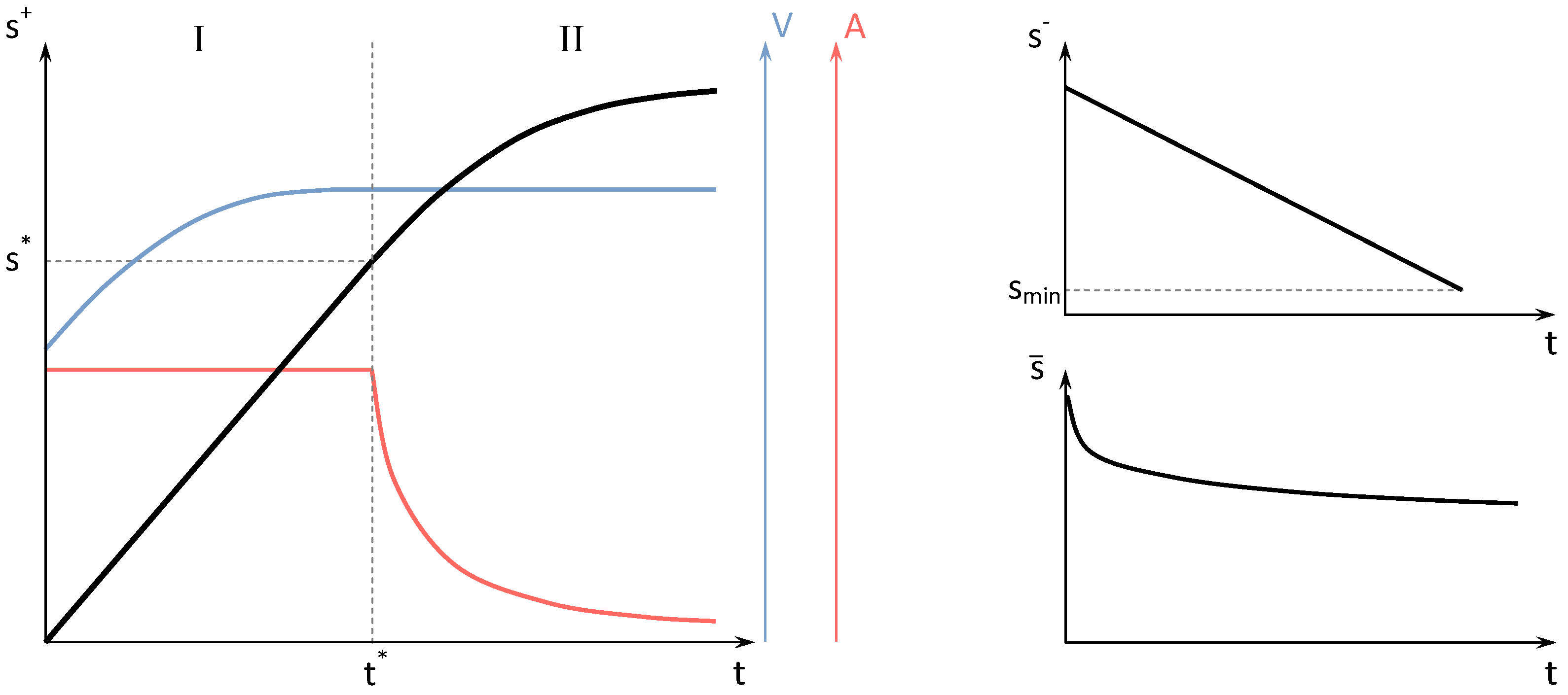
The first stage is characterised by a “constant current” process, whereas the second stage applies “constant voltage”. Within the constant current stage we have a constant charging rate , and thus linearly increase the amount of stored energy in the battery. The cell voltage is following this trend, but tapers off towards its terminal cell voltage. Let the capacity at this point be denoted by . Once this value is reached, the second stage is initiated, where the voltage is kept constant. As a result, the charging current drops off exponentially. The battery is fully charged when the charging current reaches a pre-defined value of approximately ten percent of the charging current in stage I. For the charging rate this implies that it also levels off exponentially. We summarise the change of stored energy during the two stages of the charging process by:
where is the charging efficiency with and is the maximum capacity. The parameters and are chosen such that the capacity curve and its derivatives are continuous at .
When discharging a lithium-ion battery, the operating voltage (given a fixed current) behaves as shown in [16,17]; i.e., with an almost constant value for a wide range until it drops off sharply at low capacities. According to this, we consider a constant discharging rate until a lower limit is reached
where is the discharging efficiency with . Discharging the battery below is prohibited for the user within our model (cf. Figure 1).
If the battery is neither charged nor discharged, it will still lose capacity due to self-discharging. We model the effect with an exponential decrease of the capacity
where is the self-discharging rate.
2.2. Household Demand and Load
The set of households who participate in the DSM program is denoted by . The total number of participants is . We define the energy demand of a household as the amount of energy that is needed to run all its appliances at time interval . The total daily schedule of unshiftable demand is then . This demand does not include any action of the battery.
Let denote the load, which is defined by the amount of energy that is drawn from the grid by household n at at time interval . It combines the energy demand with the amount of energy that is charged or discharged by the battery; i.e.,
where is obtained from suitable integrals of the charging and discharging curves (1) and (2). Note that for all intervals, as the amount discharged from the battery cannot be larger than the demand in the respective interval. We write for the schedule of loads and can calculate the total load on the grid at time interval by
2.3. Cost Model
We model one utility company that serves all the households in the neighbourhood. In order to incentivise the users to avoid consumption during peak hours, a time-of-use tariff is employed. The costs per energy unit is calculated separately for each interval and depends on the aggregated load of all users. Similar to [8,11,18], we want to employ a quadratic cost function ; i.e.,
where y is the aggregated load at time t given by and the coefficients , , and .
3. The Battery Scheduling Game
In this section we formulate the non-cooperative game between the households. To be more precise, we describe a battery scheduling game in which players want to minimise their energy bill by shifting loads through their respective battery usage. Here, we detail the possible actions for each participant and clarify the relation between the cost function and the utility function of the game. This is followed by an analysis of the existence of a solution. We also present the iterative algorithm that is employed to find this solution.
3.1. Game Formulation and Equilibrium Analysis
In this day-ahead scheduling game, an action of player is described by schedule of battery activities . In particular there are four options can represent per interval:
Based on (4), we can calculate a corresponding load schedule for each action . Actions are deemed unplayable if they lead to invalid battery states; i.e., charge states that do not fulfil the requirements given in Section 2. The fact that there are two possibilities to charge the battery gives more flexibility for the user.
The utility function reflects the bill player n has to pay for the upcoming day, given that they chose action , while their opponents chose the actions . Similar to [5,8], we employ a proportional billing scheme, where every player pays for the share of their consumption:
with
To sum up, we define the non-cooperative battery scheduling game , with
- the set of players ,
- , where the set consists of all valid schedules for player n, and
- , with the utility function for player n (cf. (8)).
One can show that there exists a pure Nash equilibrium (NE) for this game. The proof can be done similarly to the one in [12] (Theorem 1), due to the similarity of the structure of the utility functions, the properties of the actions sets, and the fact that the demand is bounded.
3.2. Numerical Solution
The solution to the game (i.e., a NE) is computed by a best-response algorithm (cf. Algorithm 1). Through empirical studies, we found that there are usually many different NEs for each daily configuration. This is why the algorithm contains the additional do-loop in comparison to the “myopic best-response” algorithm [19].
| Algorithm 1: Best-response algorithm for finding a pure NE based on [19] |
 |
Choosing the best NE is done by comparing the sum of the utility functions for every player. Please note that even when the existence of a pure NE is guaranteed, the algorithm might not converge to it. An additional counter variable prevents getting stuck in an infinite while-loop. Nevertheless, this exit condition was not triggered in any of our simulation runs.
4. Simulation Results and Discussion
In this section, the data set and system variables that constitute the DSM scheme with a battery scheduling game are presented. The simulation results based on these are subsequently shown and discussed.
4.1. Data and Variables
The household consumption data for all our simulations stem from the openei dataset [20]. This dataset contains 365 days of simulated hourly demand data for all TMY3-locations in the USA [21]. Details on the building models can be found in [22]. Additionally, the “Residential Energy Consumption Survey” was used to associate suitable building types with each location. There are three categories: BASE, HIGH, and LOW based on the specific attributes of the respective household [23].
For our simulations, we picked households (i.e., nine BASE, nine HIGH, and seven LOW) that are all within close vicinity to represent a small neighbourhood. In order to gain insight into seasonal effects, we chose four equally separated weeks from the data set—in particular weeks 12, 25, 38 and 51—and used it to represent the individual household demand. Nevertheless, the scheduling is done on a day-ahead basis as described in Section 3.1. To this end, we set ; i.e., consider two-hour intervals, and initialise the battery at the beginning of the week with a small random capacity. From the NE, the battery states at the end of the day can be calculated and are used as initial data for the following day.
The parameters of the battery are inspired by the Tesla Powerwall 2 [24] data sheet, and can be found in Table 1.
The efficiency variables and are calculated under the assumption that charging and discharging contribute to equal amounts towards the given round-trip efficiency of . We denote this type of battery by the “realistic” battery (RB) model. For comparisons, we also run all the simulations with an “ideal” battery (IB) model; i.e., the same storage system but with . We want to highlight that the IB still follows the proposed charging and discharging curves shown in Figure 1 and is also subject to self-discharging. Within the cost function (6), we use the coefficients $/MW, $/MW, and [25].
4.2. Results
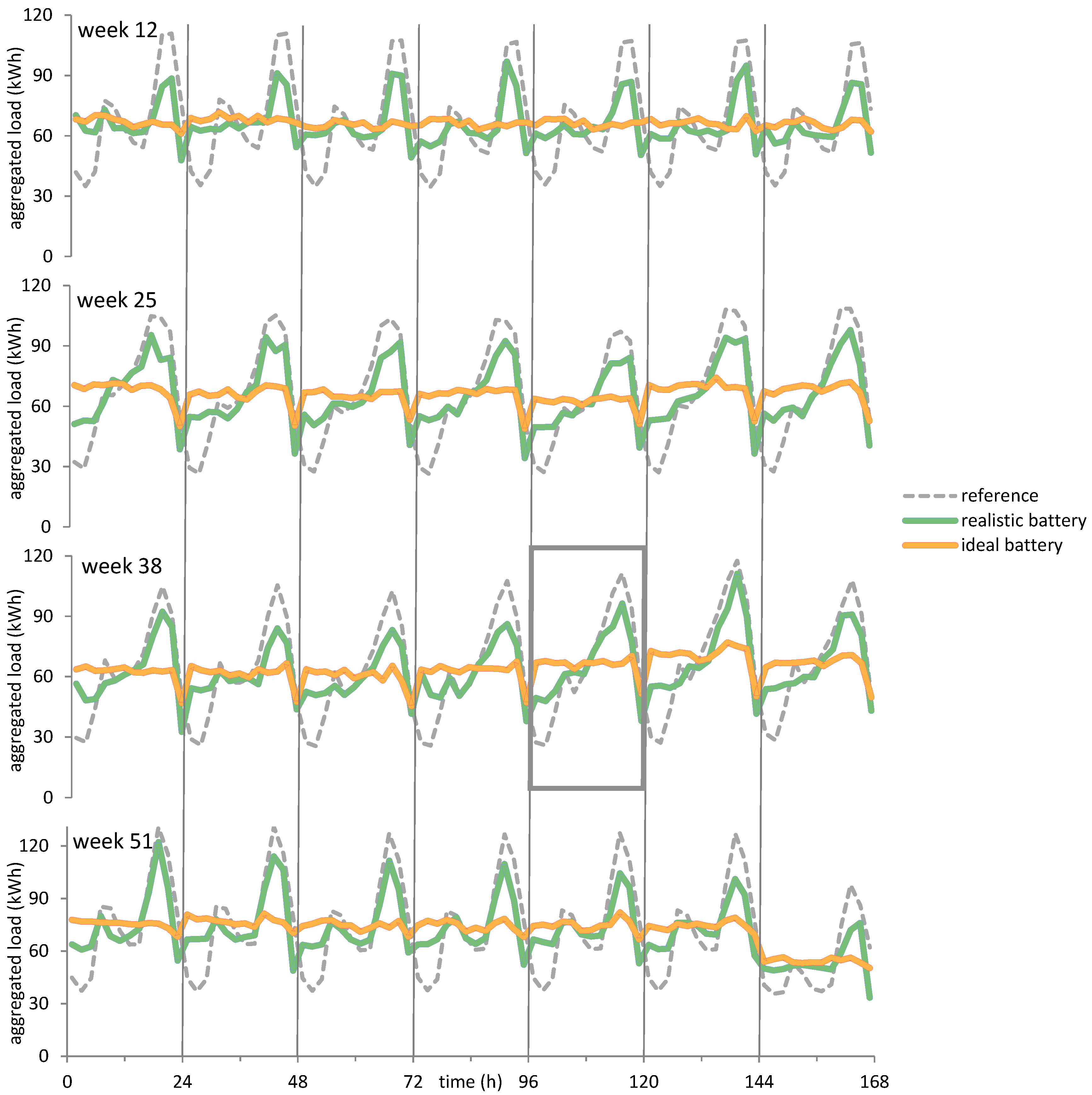
In Figure 2, the aggregated load curves resulting from playing the game with different battery models are shown—one of them with realistic parameters and the other with ideal 100% efficiency (see Section 4.1). The reference curve represents the aggregated load of the system without the battery scheduling game.
For a quantitative analysis of the load-shifting phenomenon, and since our aim is to reduce consumption during peak times, we look at the peak-to-average ratio (PAR) of the aggregated load for each individual day; i.e.,
The averages over the seven days of the respective weeks are shown in Table 2.
On average, a 14% and a 36% decrease of the PAR value was achieved by employing a game with an RB and IB model, respectively.
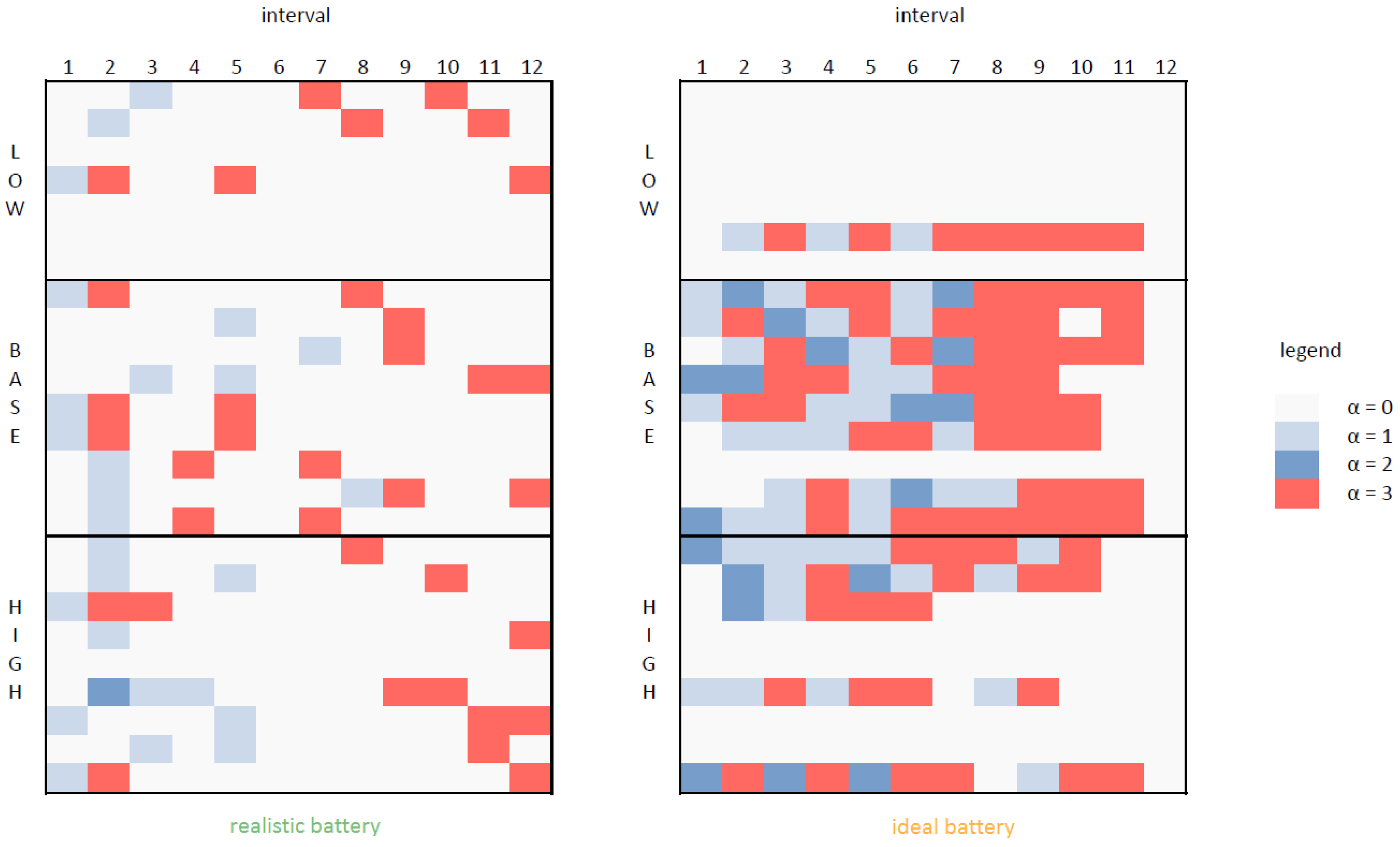
When considering the participation behaviour of the households, we look at two things: (i) the rate at which players choose to play any action other than the zero-schedule in the Nash equilibrium (cf. (7)); and (ii) the distribution of activities chosen for each individual interval. A visualisation of the schedules of a randomly chosen day (week 38, day 5) is shown in Figure 3 for both battery models. It can be seen as a representative example of the schedules for all other days. A summary for the different user classes of the participation rate and the activity distribution can be found in Table 3 and Table 4, respectively.
Table 5 shows by how much the utility function of the consumers, i.e. the energy costs for each of them, was reduced. The results for each of the four different weeks are averaged over the consumer categories for both battery models.
4.3. Discussion
4.3.1. Peak-to-Average Ratio
By playing the game the usual evening peaks of each individual day were decreased. This effect was stronger for simulation runs that apply an IB model, where an almost flat load profile was produced. Troughs are visible at the end of several days (e.g., in weeks 25 and 38) due to a finite-horizon effect that occurs when the aggregated demand during the final interval is lower than the average load in the previous intervals. This results in the players choosing to play in the respective interval, see Figure 3. As the load can only be increased by charging the battery, this would have caused an increase in costs (for this day) and thus would not have been beneficial for the players.
From our results we see the importance of the battery efficiency for reducing the PAR value. In fact, our research has shown that the cycling efficiency is the most sensitive parameter of all parameters introduced in Section 2.1 [26]. With state-of-the-art technology such as the Tesla Powerwall 2 [24], the PAR value was reduced by to . Under the assumption of an IB, PAR values close to the optimum were achieved (i.e., a reduction of ). It is worth highlighting that these results do not seem to depend on seasonal effects, as fluctuations of PAR values between the four simulated weeks were less than .
4.3.2. Participation in the Game
We observe that the participation rate was higher overall for the RB model. Nevertheless, the players who did participate in the IB scheduling game were more active; i.e., chose more activities . It becomes apparent that the lack of efficiency causes a disincentive to charge the battery for many users. While charging for shorter time periods (i.e., ) was still occasionally done during low-demand intervals, charging throughout the whole interval (i.e., ) was almost non-present in the NE schedules. None of the LOW households with an RB made use of this activity within any of the 28 simulated days (cf. Figure 3 and Table 4).
4.3.3. Utility Function
In direct relation to the smaller PAR value reduction of the game with RB model is the smaller reduction in energy costs (see Table 5). Similar to results regarding the PAR value, we observe that there seems to be no seasonal dependency. Furthermore, within each separate week, the differences between the three consumer classes is negligible. This was anticipated and intentionally pushed forward by the introduction of the proportionality factor in the utility function (8). It should be noted that the pricing scheme benefits all users whether they participate in the DSM scheme or not. A tariff that gives a higher share of savings towards the contributors might be a fairer approach.
5. Conclusions
In this paper, we proposed an advanced battery model for a DSM program: residential customers play a battery scheduling game to decrease their own costs which eventually reduce the PAR value of the aggregated neighbourhood load. The advantage of this approach is that every household can make its own decision, thereby addressing concerns of individual freedom.
It turns out that the round-trip efficiency of the storage system has an impact on the participation behaviour. In fact, it lowers the PAR reduction by more than half of what can be achieved by a system with perfect efficiency. This is accompanied by a lower reduction in energy bills for all participants. Thus, our studies underline the importance of further advancements in battery technology. One way of compensating for the imperfect efficiency of the storage system might be the introduction of a more advanced billing scheme. In the current framework, participants react to a given pricing policy, which causes a PAR reduction. In a reverse scheme, participants could be incentivised to reduce the PAR value directly and are granted cost reductions based on their respective success.
Other future research directions may include the incorporation of on-site renewable energy generation for individual participants and a thorough analysis of the life-cycle costs of the proposed system.
Acknowledgments
This work was supported by the Doctoral Training Alliance (DTA) Energy.
Author Contributions
Matthias Pilz, Luluwah Al-Fagih and Eckhard Pfluegel conceived and designed the simulations; Matthias Pilz implemented and performed the simulations; Matthias Pilz analysed the data; Matthias Pilz wrote the paper.
Conflicts of Interest
The authors declare no conflict of interest.
Abbreviations
| DSM | Demand-side management |
| PAR | Peak-to-average ratio |
| RB | Realistic battery |
| IB | Ideal battery |
| NE | Nash equilibrium |
| TMY | Typical meteorological year |
References
- Ipakchi, A.; Albuyeh, F. Grid of the Future. IEEE Power Energy Mag. 2009, 7, 52–62. [Google Scholar] [CrossRef]
- Saad, W.; Han, Z.; Poor, H.V.; Başar, T. Game-Theoretic Methods for the Smart Grid: An Overview of Microgrid Systems, Demand-Side Management, and Smart Grid Communications. IEEE Signal Process. Mag. 2012, 29, 86–105. [Google Scholar] [CrossRef]
- Pilz, M.; Al-Fagih, L. Recent Advances in Local Energy Trading in the Smart Grid Based on Game—Theoretic Approaches. IEEE Trams. Smart Grid 2017. accepted for publication. [Google Scholar] [CrossRef]
- Bayram, I.S.; Shakir, M.Z.; Abdallah, M.; Qaraqe, K. A Survey on Energy Trading in Smart Grid. In Proceedings of the 2014 IEEE Global Conference on Signal and Information Processing, Atlanta, GA, USA, 3–5 December 2014; pp. 258–262. [Google Scholar]
- Soliman, H.M.; Leon-Garcia, A. Game-Theoretic Demand-Side Management With Storage Devices for the Future Smart Grid. IEEE Trans. Smart Grid 2014, 5, 1475–1485. [Google Scholar] [CrossRef]
- Ma, K.; Hu, S.; Yang, J.; Dou, C.; Guerrero, J. Energy Trading and Pricing in Microgrids with Uncertain Energy Supply: A Three-Stage Hierarchical Game Approach. Energies 2017, 10, 670. [Google Scholar] [CrossRef]
- Celik, B.; Roche, R.; Bouquain, D.; Miraoui, A.; System, A.P. Coordinated Neighborhood Energy Sharing Using Game Theory and Multi-Agent Systems. In Proceedings of the PowerTech, 2017 IEEE Manchester, Manchester, UK, 18–22 June 2017. [Google Scholar]
- Mohsenian-Rad, H.; Wong, V.W.S.; Jatskevich, J.; Schober, R.; Leon-Garcia, A. Autonomous Demand-Side Management Based on Game-Theoretic Energy Consumption Scheduling for the Future Smart Grid. IEEE Trans. Smart Grid 2010, 1, 320–331. [Google Scholar] [CrossRef]
- Wang, Y.; Saad, W.; Mandayam, N.B.; Poor, H.V. Load Shifting in the Smart Grid: To Participate or Not? IEEE Trans. Smart Grid 2015, 7, 2604–2614. [Google Scholar] [CrossRef]
- Haider, H.T.; See, O.H.; Elmenreich, W. Dynamic Residential Load Scheduling Based on Adaptive Consumption Level Pricing Scheme. Electric Power Syst. Res. 2016, 133, 27–35. [Google Scholar] [CrossRef]
- Yaagoubi, N.; Mouftah, H.T. User-Aware Game Theoretic Approach for Demand Management. IEEE Trans. Smart Grid 2015, 6, 716–725. [Google Scholar] [CrossRef]
- Nguyen, H.K.; Song, J.B.; Han, Z. Distributed Demand Side Management with Energy Storage in Smart Grid. Ieee Trans. Parallel Distrib. Syst. 2015, 26, 3346–3357. [Google Scholar] [CrossRef]
- Mohsenian-Rad, H. Optimal Bidding, Scheduling, and Deployment of Battery Systems in California Day-Ahead Energy Market. IEEE Trans. Power Syst. 2016, 31, 442–453. [Google Scholar] [CrossRef]
- Longe, O.M.; Ouahada, K.; Rimer, S.; Harutyunyan, A.N.; Ferreira, H.C. Distributed Demand Side Management with Battery Storage for Smart Home Energy Scheduling. Sustainability 2017, 9, 120. [Google Scholar] [CrossRef]
- Luo, X.; Wang, J.; Dooner, M.; Clarke, J. Overview of Current Development in Electrical Energy Storage Technologies and the Application Potential in Power System Operation. Appl. Energy 2015, 137, 511–536. [Google Scholar] [CrossRef]
- Richtek. Designing Applications with Li-ion Batteries. Available online: http://www.richtek.com/battery-management/en/designing-liion.html (accessed on 1 June 2017).
- IBT Power. Typical Lithium Ion Technical Data. Available online: http://www.ibt-power.com/Battery_packs/Li_Ion/Lithium_ion_tech.html (accessed on 1 June 2017).
- Misra, S.; Bera, S.; Ojha, T.; Zhou, L. ENTICE: Agent-Based Energy Trading with Incomplete Information in the Smart Grid. J. Netw. Comput. Appl. 2015, 55, 202–212. [Google Scholar] [CrossRef]
- Shoham, Y.; Leyton-Brown, K. Multiagent Systems, 1st ed.; Cambridge University Press: Cambridge, UK, 2009; p. 484. [Google Scholar]
- U.S. Department of Energy. Commercial and Residential Hourly Load Profiles for All TMY3 Locations in the United States; U.S. Department of Energy: Washington, DC, USA, 2013.
- NREL. User Manual for TMY3 Data Sets; NREL: Golden, CO, USA, 2008.
- U.S. Department of Energy. Building America House Simulation Protocols; U.S. Department of Energy: Washington, DC, USA, 2010.
- U.S. Department of Energy. Building Characteristics for Residential Hourly Load Data; U.S. Department of Energy: Washington, DC, USA, 2013.
- Tesla. Tesla Powerwall 2. Available online: https://www.tesla.com/en_GB/powerwall (accessed on 5 June 2017).
- Rahbar, K.; Xu, J.; Zhang, R. Real-Time Energy Storage Management for Renewable Integration in Microgrid: An Off-Line Optimization Approach. IEEE Trans. Smart Grid 2015, 6, 124–134. [Google Scholar] [CrossRef]
- Pilz, M.; Al-Fagih, L. A Parameter Analysis of Residential Storage Systems for Home Energy Scheduling. 2017; work in progress. [Google Scholar]
Figure 1.
Schematic illustration of the charging and discharging behaviour of a lithium-ion battery. (left) Two-stage charging process plotted over time t. State of capacity in black, voltage V in blue, and current A in red. (top right) State of capacity during discharging over time t. (bottom right) State of capacity due to self-discharging.

Figure 2.
Aggregated load curves over four different one-week periods; i.e., week 12, week 25, week 38, week 51 in the data set [20]. For each week, the results for not playing the game (reference) can be compared to the results obtained from playing the game with either a realistic battery or an ideal battery model. For week 38, day 5 is highlighted in reference to the results shown in Figure 3.

Figure 3.
Illustration of Nash equilibrium for the scheduling game at day 5 in week 38. Each row represents a schedule (i.e., a set of options—one for each interval; cf. (7)), chosen by the respective player. On the left, the results under consideration of a realistic battery model are shown, whereas on the right an ideal battery model is applied.


Table 1.
Parameters for a Tesla-inspired [24] home battery storage system used throughout all simulations runs labelled with “RB model”.
Table 1.
Parameters for a Tesla-inspired [24] home battery storage system used throughout all simulations runs labelled with “RB model”.
| Variable | Value |
|---|---|
| kW/h | |
| kW/h | |
| kWh | |
| kWh | |
| kWh |
Table 2.
Peak-to-average ratios calculated as the average over the individual days of week 12, week 25, week 38, and week 51 for the case without storage system (Reference) and both battery models. gives the average over all four weeks. IB: “ideal” battery; RB: “realistic” battery.
Table 2.
Peak-to-average ratios calculated as the average over the individual days of week 12, week 25, week 38, and week 51 for the case without storage system (Reference) and both battery models. gives the average over all four weeks. IB: “ideal” battery; RB: “realistic” battery.
| Reference | RB Model | IB Model | ||
|---|---|---|---|---|
| Period | w12 | |||
| w25 | ||||
| w38 | ||||
| w51 | ||||
Table 3.
Comparison of participation rates depending on the battery model and consumption category. Results are obtained by averaging over all weeks.
Table 3.
Comparison of participation rates depending on the battery model and consumption category. Results are obtained by averaging over all weeks.
| RB Model | IB Model | ||
|---|---|---|---|
| Category | LOW | ||
| BASE | |||
| HIGH |
Table 4.
Occurrence of different activities within the equilibrium schedules for different player categories and both battery models. Results are obtained by averaging over all weeks.
Table 4.
Occurrence of different activities within the equilibrium schedules for different player categories and both battery models. Results are obtained by averaging over all weeks.
| RB Model | IB Model | ||||||||
|---|---|---|---|---|---|---|---|---|---|
| Category | LOW | ||||||||
| BASE | |||||||||
| HIGH | |||||||||
Table 5.
Amount of reduction of the utility function (i.e., energy costs). Results averaged over the different consumption categories are shown for each week together with an overall average .
Table 5.
Amount of reduction of the utility function (i.e., energy costs). Results averaged over the different consumption categories are shown for each week together with an overall average .
| RB Model | IB Model | ||||||
|---|---|---|---|---|---|---|---|
| LOW | BASE | HIGH | LOW | BASE | HIGH | ||
| Period | week 12 | ||||||
| week 25 | |||||||
| week 38 | |||||||
| week 51 | |||||||
© 2017 by the authors. Licensee MDPI, Basel, Switzerland. This article is an open access article distributed under the terms and conditions of the Creative Commons Attribution (CC BY) license (http://creativecommons.org/licenses/by/4.0/).
Share and Cite
MDPI and ACS Style
Pilz, M.; Al-Fagih, L.; Pfluegel, E. Energy Storage Scheduling with an Advanced Battery Model: A Game–Theoretic Approach. Inventions 2017, 2, 30. https://doi.org/10.3390/inventions2040030
AMA Style
Pilz M, Al-Fagih L, Pfluegel E. Energy Storage Scheduling with an Advanced Battery Model: A Game–Theoretic Approach. Inventions. 2017; 2(4):30. https://doi.org/10.3390/inventions2040030
Chicago/Turabian StylePilz, Matthias, Luluwah Al-Fagih, and Eckhard Pfluegel. 2017. "Energy Storage Scheduling with an Advanced Battery Model: A Game–Theoretic Approach" Inventions 2, no. 4: 30. https://doi.org/10.3390/inventions2040030