1. Introduction
Once limited to the domain of elite athletes, wearable devices are increasingly used by the general public for health and wellness monitoring ranging from clinical rehabilitation to activity (e.g., running or swimming) tracking. These devices have made it possible to continuously monitor not only daily activities, but also heart rate, skin temperature, breathing rate and many other physiological, as well as environmental parameters. Due to the rapid technological advancements in sensor technologies, vast amounts of raw data streams are being generated, which justifies the need for new methods to analyze these data and provide valuable feedback to the user. Most fitness devices available provide simple alerts, such as reminding a person to be active or to practice deep breathing if their heart rate is too high, thus providing vital feedback for not only fitness training, but also as indicators of medical conditions.
It is evident that continuous monitoring of physiological responses is beneficial, while forecasting or predicting these quantities into the future can be also advantageous. For example, in endurance training, knowing ahead of time what your heart rate and breathing rate will be a minute into the future can allow the individual to maintain a desired intensity level for their workout. In the medical field, if a person suffers from asthma, then predicting his/her total exposure to particulate matter based on their prediction of air volume intake may be used by the individual to decide whether to keep performing a particular activity, slow down or even go indoors. Furthermore, prediction of these physiological quantities can be used to determine anomalies in an individual’s response by capturing how it deviates from the expected values. However, predicting physiological responses into the future can be a challenging problem since there are a number of factors that need to be taken into account including: physical activities, environmental factors (e.g., temperature, humidity, ozone levels) and cognitive and affective factors (e.g., stress levels). Furthermore, as continuous monitoring using wearable devices becomes ubiquitous, we anticipate predictive models that are personalized to each individual will become more essential to characterize what is normal for a particular individual as opposed to the norm for the population.
In this article, we focus on the analysis of the effect of physical activities on the prediction of physiological responses. We consider stationary activities, transition activities (transitions between activities) and complex activities of daily life. Activities are executed at varying paces due to inter subject variability. Data are captured from individuals in a controlled environment (in order to reduce the effect of environmental and cognitive/affective factors) while performing high level activities of daily life such as setting up a table, moving objects and typing a document; and exercise activities such as riding a bicycle, walking on a treadmill and rowing. Our aim is to learn the strength and weaknesses of predictive techniques on these controlled environments while performing continuous monitoring during the execution of complex activities and their transitions. In this study, we focus on the prediction (up to 60 s into the future) of heart rate and respiratory rate as a case study. However, this methodology can be extended to other physiological measurements such as blood pressure, minute ventilation or energy expenditure. The main contributions of this work include:
The introduction of a new dataset that incorporates physiological and activity information while performing activities of daily life (see
Figure 1 for a snapshot of the data);
Introducing a methodology for quantifying the accuracy of predictive algorithms for heart rate and respiratory rate under varying physiological activities and using different predictors;
Studying the performance of various prediction approaches for physiological responses;
Studying the effect of predictors that incorporate historical information of physiological parameters for prediction;
Studying the effect of the forecast window size (i.e., how far into the future we predict responses) on prediction accuracy;
Studying the effect of activity clustering for prediction of physiological responses.
We focus on the regression problem using a single window of historical values. However, this framework can provide the building blocks for time series analysis when longer datasets are available to enable proper validation and testing of these approaches.
As an outcome of this study, we verified that it is possible to forecast (up to 60 s into the future) heart rate and respiratory rate using personalized models for individuals in scenarios with complex activities and dynamic transitions without the effect of environmental or cognitive/affective factors. Furthermore, it is observed that activity clustering does improve the predictive power in our dataset when performing predictions across different modalities (i.e., using heart rate to predict breathing rate, or vice versa). Linear models seems to be sufficient when considering regression that includes prior measurements of the same modalities.
This article is organized as follows: materials and methods are discussed in
Section 2, results and discussion are presented in
Section 3; and conclusions and future work are listed in
Section 4.
2. Materials and Methods
In this Section we discuss background on the relationship between heart rate, respiratory rate and physical activities in
Section 2.1. We present our data collection efforts in
Section 2.2, followed by the pre-processing and alignment of different data streams in
Section 2.3. In
Section 2.4, we discuss our proposed pipeline for forecasting.
2.1. Relationship between Heart Rate, Respiratory Rate and Physical Activity
In this subsection, we discuss the importance of heart rate and respiratory rate for health monitoring applications and provide some references to known relationships between these parameters. For this study, we do not aim to discover new relationships, but to quantify how well existing algorithms can capture these relationships in order to provide accurate physiological response prediction. The tools presented in this study can also be used to identify new relationships across other sensing modalities.
For most fitness [
1,
2] and medical [
3] applications, heart rate and breathing rate are important and commonly measured quantities. In the medical field specifically, monitoring of physiological signals is routine. While heart rate is commonly measured, respiratory rate is not frequently recorded due to the cumbersome equipment and the discomfort that it causes to the patient [
4,
5]. As an alternative to respiratory rate measurements, pulse oximetry is used, which actually is not an appropriate substitute [
4]. For example, pulse oximetry is inaccurate in low perfusion states and does not provide information of hemoglobin level, efficiency of oxygen delivery or adequacy of ventilation [
6].
Apart from clinical environments, monitoring physiological responses during everyday life is also beneficial. For example, one of the most obvious and straightforward signs of asthma is the abnormal increase of respiratory rate [
3]. In many cases, an abnormal change of respiratory rate is not easily noticed before it gets worse as time goes on, which further signifies the importance to daily monitoring of this quantity for people who have such pre-existing conditions. Besides preventing potential chronic illness, monitoring physiological signals in the mobile environment is also helpful for either fitness-oriented or professional physical training. The respiratory rate is also a reliable marker of anaerobic threshold, which is important to measure the progress of endurance athletes and to plan training regime programs [
7,
8].
It is known that physical activities have an effect on the heart rate [
9,
10]. Prior work in heart rate prediction based on physical activities [
11] further highlights the relationship between heart rate and physical activities. Studies have also shown a good correlation between heart rate, ventilation and oxygen consumption [
12,
13]. Some studies use minute ventilation as a predictor of cardiac heart failures [
14,
15]. It is however difficult to measure ventilation in field studies. Prior studies [
12,
16] have addressed this limitation by estimating ventilation using heart rate, which can be easily monitored by a portable heart rate monitor.
2.2. NCSU-ADL Dataset
This subsection introduces the dataset recorded for this study. As discussed in
Section 1, we aim to predict physiological responses in realistic scenarios. Our dataset focuses on capturing physiological signal and motion information of individuals in scenarios with complex activities and dynamic transitions without the effect of environmental and cognitive/affective factors.
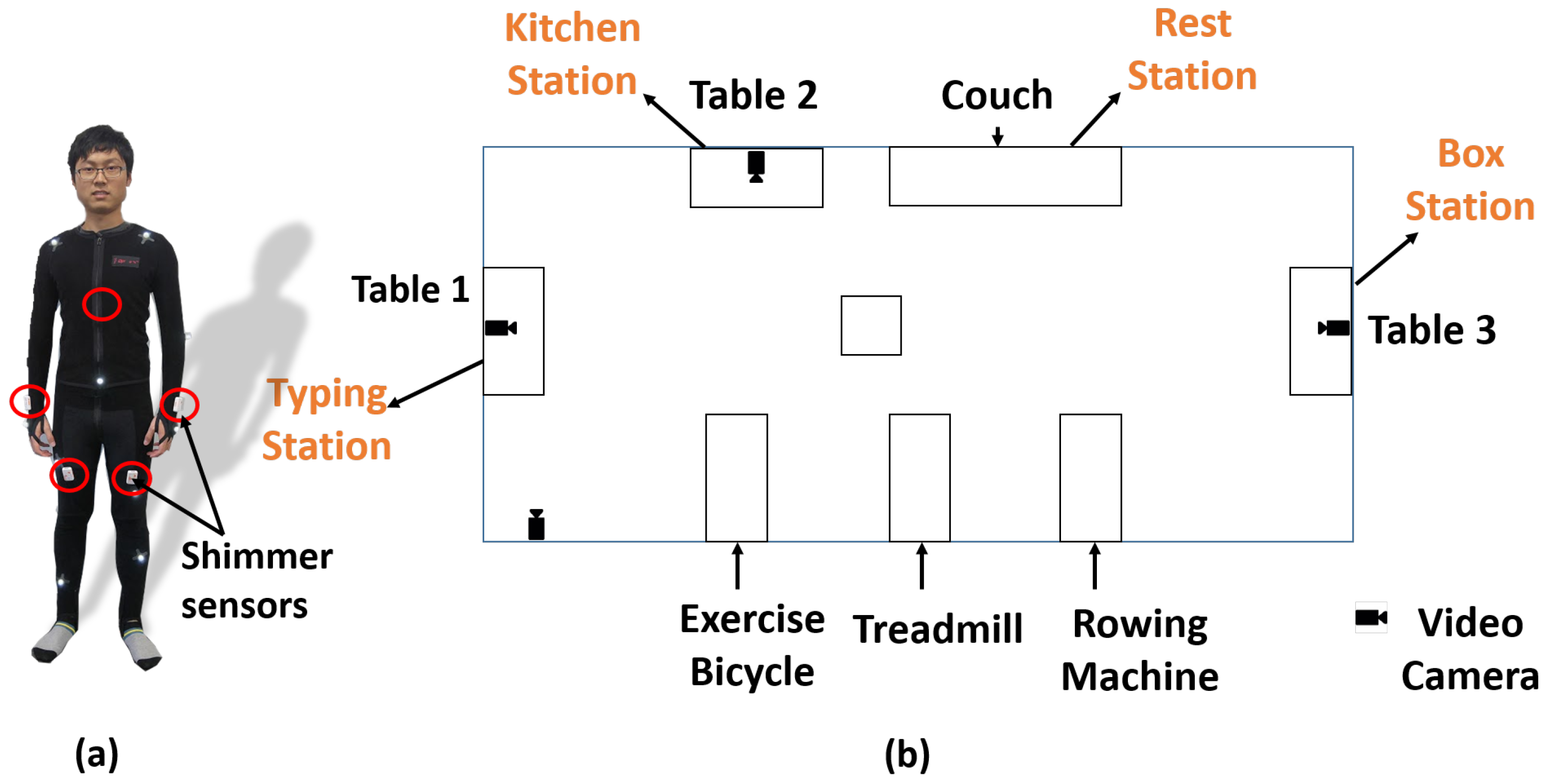
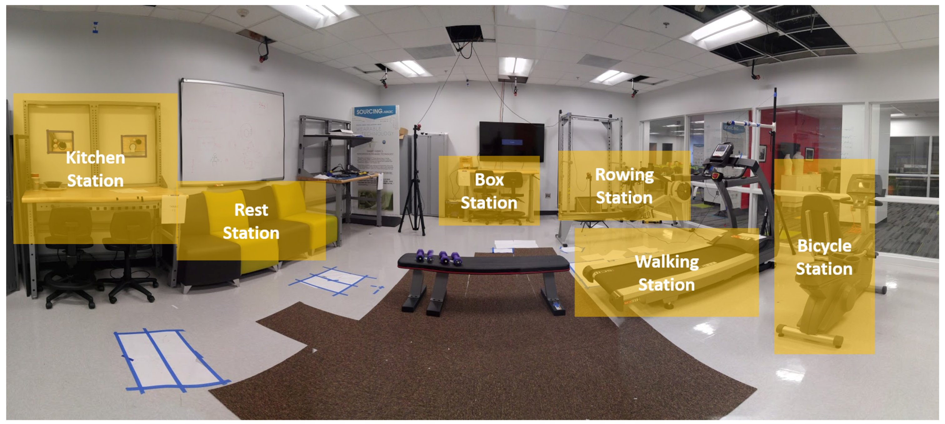
The data collection was undertaken at North Carolina State University (NCSU) under Institutional Review Board (IRB) 7799. All participants in the study were healthy individuals in the age group ranging from 18–30 years old. We collected data from 10 volunteers. The layout of the space where all the activities were performed is shown in
Figure 2 and a panoramic view of the space in
Figure 3. We focus on activities of daily life (ADL), including periodic (e.g., walking, bicycling), non-periodic (e.g., setting up a dinner table) and stochastic (e.g., typing a document). The participants had to undergo a 2-h session for training, placing sensors and data collection (approximately 1 h). The following tasks were included in the protocol:
Row on a rowing machine
Move a 20-lb object from one table to another
Ride an exercise bicycle
Rest on a chair for three minutes
Set up dinner and clean up the table
Walk on the treadmill
Drink water
Type a one-page document
Lie down for three minutes
In order to ensure that we capture enough transitions between the different activities, the participants were asked to perform short activities (e.g., moving a 20-lb object) four times throughout the protocol and longer activities (e.g., walking on the treadmill) two times. Participants were also asked to perform complex activities such as typing a document or setting up a dinner table at their own pace. The first half of the protocol was the same as the second half of the protocol. This was done so we can use the first half for training and the second for prediction in order to mimic more realistic scenarios in which only historic information is available to predict future instances. The sensors used for data collection are:
BioHarness: This sensor [
17] is an off-the-shelf sensor that can measure subject’s heart rate (beats per minute), breathing rate (breaths per minute), acceleration (g), skin temperature (
C) and activity levels. This device has an adjustable chest strap, and it is worn by the volunteer throughout the data collection process. We collected accelerometer, EKG (electrocardiogram) and breathing rate. The sampling rate was 100 Hz, 250 Hz and 25 Hz, respectively.
Shimmer Platform: Each sensor in this platform [
18] contains an off-the-shelf inertial measurement unit, which has a three-axis low-noise accelerometer, a three-axis gyroscope and a three-axis magnetic sensor, which measures acceleration, orientation and magnetic field, respectively. Five of these devices were worn: two on the wrists, two on the legs and one on the chest. The sampling rate for these devices was set to 202 Hz. In addition to the IMU unit, the Shimmer sensor [
18] on the chest can record EKG signals. We use this sensor to record the EKG measurements at a sampling rate of 202 Hz.
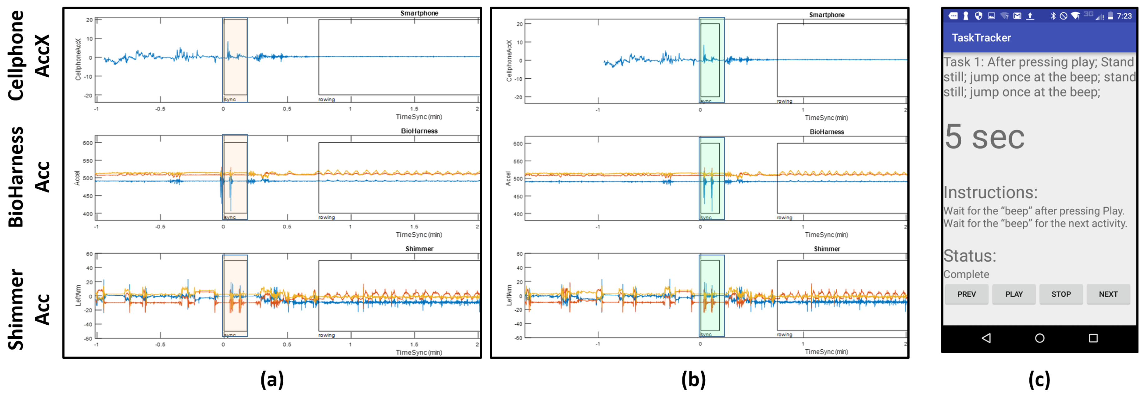
Smartphone: A Motorolla Moto E (2nd Generation) was used in the experiment to give instructions to the user. The user was given instructions through an application called TaskTracker (see
Figure 4 for a snapshot). This tool was developed in house. The user interacts with the protocol by pressing “Next”, “Play”, “Stop” or “Previous”. If something goes wrong during an ongoing segment, the user can press “Previous” to go back to the last segment. The app beeps when the task starts or ends and also includes a countdown timer for certain instructions. This helped us to sync between activities and also allows the participant to move at his/her own pace and indicate when the activity is complete and he/she ready to move on to the next task. The interactions with the app are stored locally and used as ground truth for the activity labels. We also use an application called ScienceJournal [
19] to record the phone’s accelerometer data (
x,
y and
z axes) for alignment purpose.
For this study, we use the respiratory and heart rate measurements from the BioHarness sensor and accelerometer data from Shimmer sensors. We also use the accelerometer data from the smartphone and BioHarness sensor, but only for data alignment purpose; this is discussed in
Section 2.3. Prior studies have used smartphone accelerometer data and have shown that even though it is possible to do activity recognition with smartphone data, they are not suitable for activities and motions that incorporate upper limb motion [
20]. Motion artifacts (caused due to movement of the sensor while recording) and poor contact of the sensor can influence the heart rate and respiration rate measurements, thus making them unusable in the analysis. According to [
2,
21], the BioHarness was found to provide reasonably accurate heart rate and respiratory rate measurements during exercises of varying intensity. In our experiments, we noticed consistent good signal quality when the sensor was properly secured to the individual. However, several individuals had low quality signals with motion artifacts when the BioHarness had poor contact with the skin. Due to this issue, only the data from five subjects are used for this study.
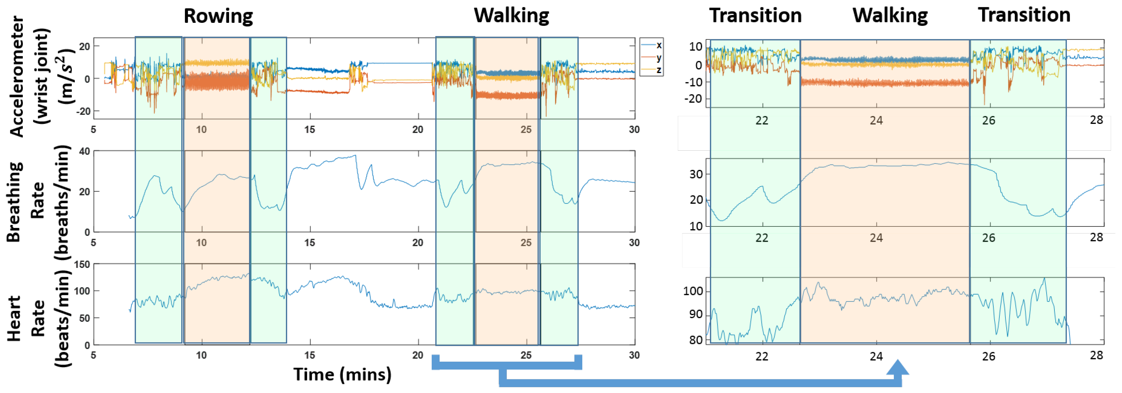
Figure 1 shows a snapshot of the different data streams that are used. The figure also highlights transition regions; these are the times when a subject was switching between activities. It is worth pointing out that the physiological quantities vary during these transition regions; we can see for instance a clear drop in heart rate and respiration rate in the highlighted green regions in
Figure 1.
2.3. Data Alignment
Data alignment is a key step in analyzing multi-modal data streams. We use the smartphone accelerometer data to align the different data streams. The protocol followed by the subject has a start and end sequence where he/she were asked to jump two times, so that the jumps are captured in the accelerometer data on all the devices. These spikes appear at the beginning and the end of the protocol.
Figure 4a shows the spikes (highlighted in orange) at the beginning of the protocol before alignment. We see that the spikes from the jumps are evident, but they are slightly off from each other due to time misalignment; notice the automatically picked boxes show peaks, but they are not exactly aligned. In order to fix this, we manually align these streams. We aligned the signals using the highest peak on the accelerometer values, which we associated with the instance in which an impact with the ground was recorded. Since the sensors were located at different parts of the body, this could lead to additional offsets not considered by this alignment process. However, even in this case, we do not expect offsets greater than 100 milliseconds. Since the features extracted for this study use windows in the order of seconds and tens of seconds, then we do not consider this a big source of error for our analysis. The highlighted regions in
Figure 4b show the outcome of this manual alignment.
Figure 4c shows an example of one set of instructions in the protocol given to the participant by the TaskTracker app. Annotations of the data streams for data retrieval are produced automatically from the log files generated by TaskTracker. The NCSU-ADL data and details of its content can be found in the provided website [
22].
2.4. Methodology for Forecasting
For this study, we focus on personalized models since physiological responses are known to greatly vary across individuals, which is also observed in our dataset. We consider scenarios in which individuals wear sensing devices for a period of time in order to provide enough data to train models that can later be used for forecasting physiological responses into the future. As an illustration, let us consider an individual that has a device that measures respiratory and heart rate and a separate device that only measures heart rate. In the proposed framework, we can record data from the first device (which has both sensing modalities) for a period of time, and then provide predictions into the future for respiratory and heart rate when the user is using either one of these devices. As more data are collected from the user, these models can be improved by re-training the models in a smartphone platform or the cloud.
In the rest of this subsection, we discuss our pipeline to forecast physiological responses (see
Figure 5). Features extracted from the accelerometer data are projected to a lower dimension via locally linear embedding (LLE); this is a dimension reduction technique (discussed in
Section 2.4.1). Unsupervised clustering is then performed on these lower dimensional features to group similar activities together (discussed in
Section 2.4.2). Windows in the past of physiological sensor data, namely breathing rate and heart rate, are extracted and used to create models for each cluster (discussed in
Section 2.4.3). We propose an ensemble approach for forecasting of physiological responses by incorporating activity information from multiple scales (discussed in
Section 2.4.4). For every test point, we repeat a similar procedure of extracting features and windows to find which cluster it belongs to and further use the model trained for that particular cluster to forecast these physiological quantities. We use standard evaluation metrics (discussed in
Section 2.4.5) for analysis of the models. Different components of the pipeline are described in the following sub-sections.
2.4.1. Extracting Features and Windows of Data
In this subsection, we go over how windows of data and features are extracted for activity clustering and training our predictive models. First, a brief overview of activity recognition is presented.
Real-time activity recognition has been widely studied in the past, and the most commonly-used feature extraction techniques rely on a sliding window-based approach for extracting various statistical, time-domain, frequency-domain and time-frequency features [
23,
24,
25]. The effect of window length on classification accuracy has been studied in the past [
26,
27,
28,
29,
30], suggesting optimal values ranging from 0.25–12.8 s [
31,
32,
33]. However, a single fixed window size might not work best for all activities [
31,
34], so a dynamically-varying window size was proposed in [
35,
36]. Furthermore, window size affects computational cost and thus power consumption; a major concern in wearable sensors computing [
37,
38,
39], especially for multi-modal data streams.
For our application, choosing an optimal window size
translates to extracting features that properly discriminate between activities at the right temporal scale. It is desirable to have similar activity clusters close to each other, while dissimilar activities farther away. In order to select the values of
and
, we performed an analysis similar to the one presented in our prior work [
40]. In this work, a classifier is used to determine the pair
that yields the best F1 score for activity recognition. This classifier combines activity label predictions from features using either
or
window sizes via a maximum likelihood approach. These values for
are also consistent with the range between 0.25 and 12.8 s, which has been previously reported in the literature for best classification [
31,
32,
33]. Therefore, we use values obtained from this analysis:
s and
s.
We use acceleration data from one leg and one wrist sensor; this ensures that we capture both upper and lower body activities (e.g., bicycling will be captured by the leg sensor and drinking water will be captured by the wrist sensor). Specifically, in our analysis, we use acceleration data from the left wrist and right leg. Time domain features extracted for each joint are the mean, variance, skewness, kurtosis and correlation between the axis (xy, yz and xz); frequency domain features are mean power spectral density and peak power spectral density. The dimensionality of the feature set was 42; this was reduced using locally linear embedding to dimension 3.
These multi-modal data streams have different sampling rates, i.e., the numbers of data points per stream are different. We interpolated the heart rate and breathing rate to 1 Hz. Interpolation is necessary in order to have data points for all time values used to make predictions. Raw breathing rate and heart rate were extracted over windows in the past () of size 20, 30, 40 and 50 s and used as predictors to assess the impact of the different sizes of windows on the forecasting results.
2.4.2. Unsupervised Clustering of Activities
Unsupervised clustering was performed on the reduced acceleration features using the revised DBSCAN (density-based spatial clustering of applications with noise) method [
41], which is more robust to the issue of border objects than the original DBSCAN [
42]. The clustering radius
is used in a hierarchical fashion. We start with a small radius and increase it gradually until we reach an
at which all points belong to the same cluster. The
range chosen during these experiments was 0.0002–0.06.
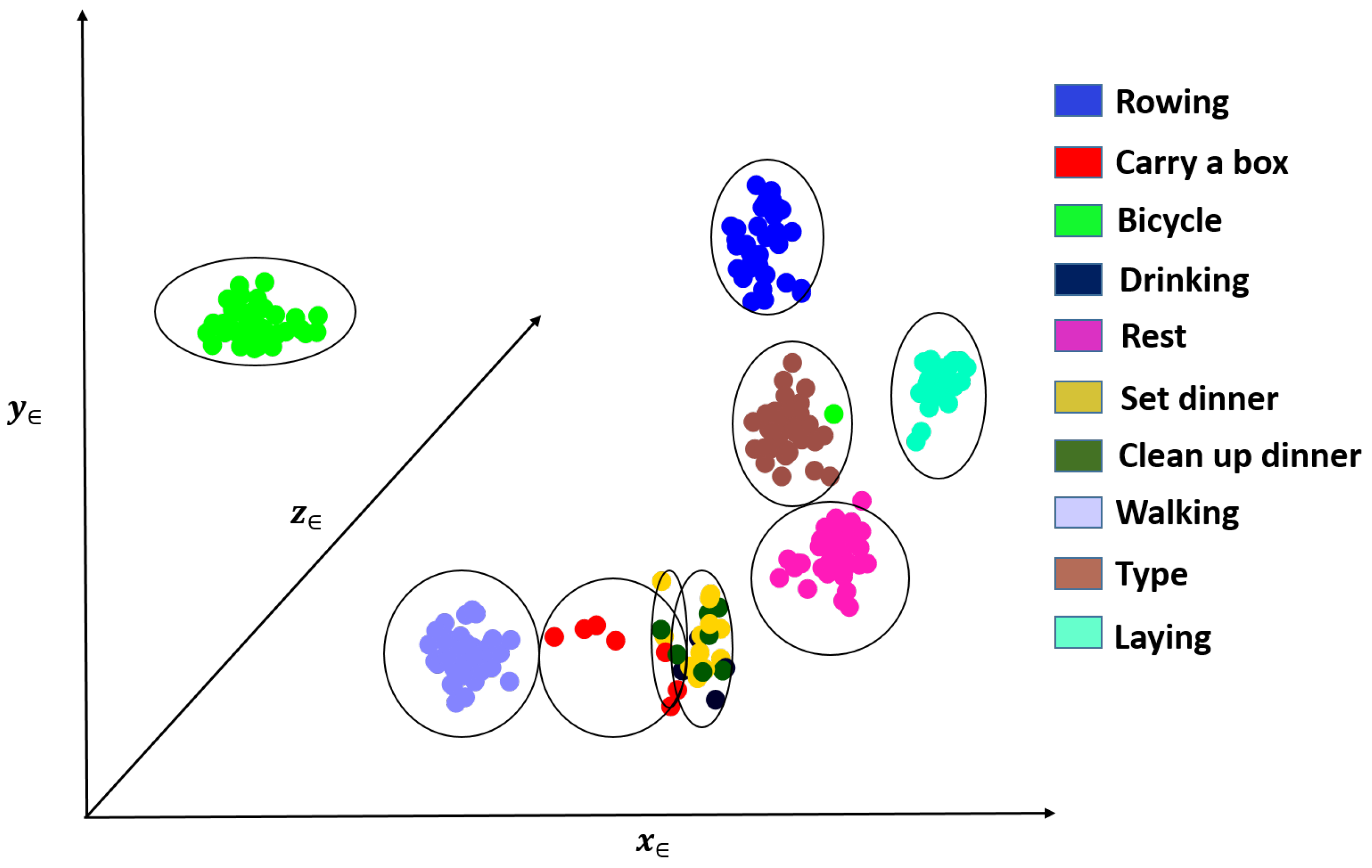
Figure 6 shows an example of one such clustering for a fixed
value. We colored points using the manual activity labels for visualization purposes only. We can see that similar activities are clustered close together, and dissimilar ones are far away from each other.
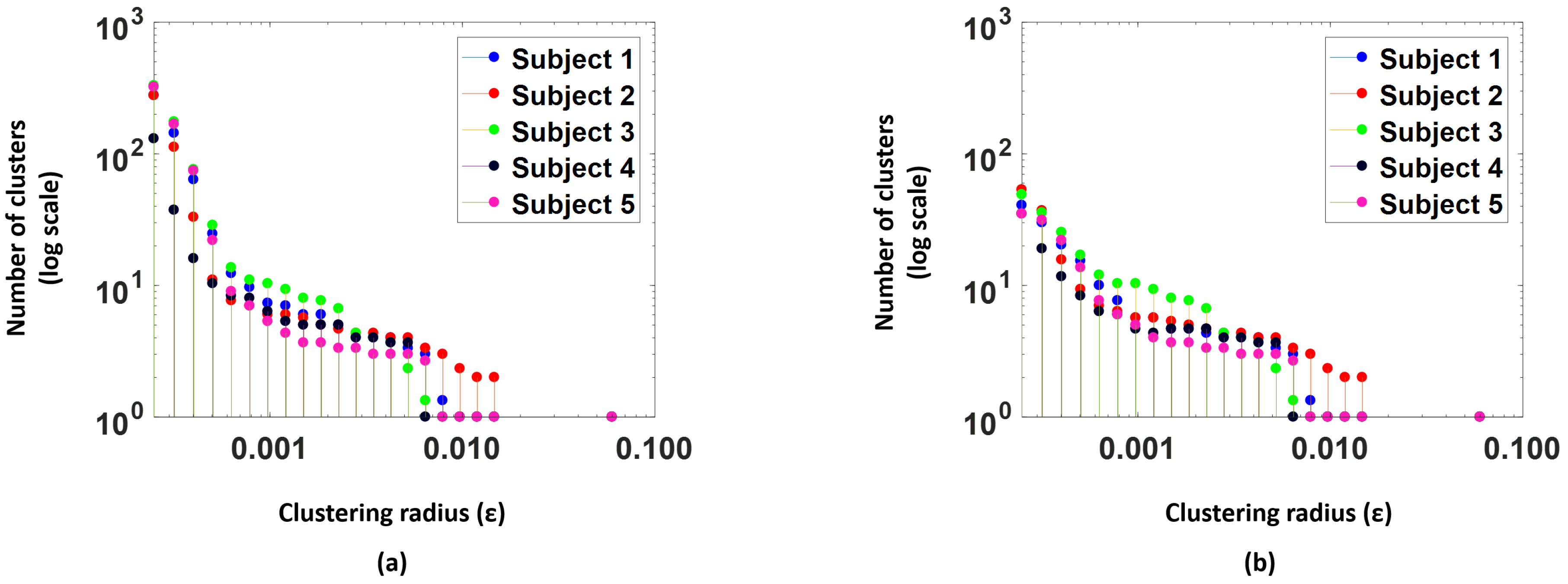
The clustering radius governs the number of clusters in a level of the hierarchy. Small values of
(radius parameter) have a larger number of clusters, but as the
increases, some of these clusters start merging with others to create more compact clusters.
Figure 7a, shows number of clusters (log scale) versus the clustering radius for the 5 subjects in the study. We see that as the
value increases the number of clusters drops.
We choose an unsupervised methodology to address real-time scenarios when it is not feasible to manually segment and label activities. Activity-aware models have been used in the context of energy expenditure in [
43]; the authors generate activity clusters using unsupervised clustering to accurately estimate energy expenditure. Inspired by this idea, we decided to use unsupervised clustering to group activities into different categories. Moreover, for predicting physiological parameters, recognizing exactly which activities the subjects are performing is unnecessary; however, it may be helpful to cluster activities with similar movement properties (e.g., intensity or pattern) because similar movements might have a similar effect on physiological responses.
2.4.3. Learning Models
Modeling physiological signals has drawn considerable attention in the past 30 years. Numerous studies have studied the relationship among different physiological responses and physical activities. For example, Xiao et al. [
11] take advantage of physical activities data to forecast the heart rate with the evolutionary neural network. However, few studies have focused on real-time respiratory rate forecasting using activity information, although it is well understood that physical activities have a significant effect on respiratory rate [
44].
In our forecasting pipeline, we adopt an SVM regression model with a Gaussian kernel. The kernel scale was decided using a heuristic procedure provided by MATLAB when the corresponding parameter is set to be “auto”. We also perform an analysis by replacing the SVM regression model with a simple linear model to further analyze the relationship between predictors.
Any clusters that have less than 5 points are considered as outlier clusters and are excluded from the training procedure.
Figure 7b, illustrates the number of clusters actually used for training models after the outlier clusters are removed; we observe that the number of clusters reduces significantly. Models are trained per cluster to forecast for a period
30 and 60 s for
and
(window parameters for activity clustering). The predictions for a future data point at
are made based on the data from
. The range of
depends on the application of interest. Models were trained for the following scenarios:
Predicting breathing rate when breathing rate is measured: This scenario is of interest when a device such as a chest strap with a breathing rate sensor is worn by the subject.
Predicting breathing rate with heart rate measurements only: Most of the wearable devices available today measure heart rate, but not respiratory rate. This model then is useful when we do not have a chest strap.
Predicting breathing rate with heart rate and breathing rate measurements: This model uses a combination of both breathing rate and heart rate, when both quantities are available from the sensors. This model was specifically trained to determine if past heart rate values were helpful to forecast breathing rate.
Predicting heart rate when heart rate is measured: Heart rate is the most commonly-measured quantity by fitness devices; this model forecasts heart rate.
Predicting heart rate with breathing rate measurements only: This model was designed when the heart rate is not available, but the breathing rate is measured. We consider this model for completeness of our analysis even though we anticipate that most scenarios will have heart rate accessible, as well.
Predicting heart rate with heart rate and breathing rate measurements: This model uses a combination of both breathing rate and heart rate, when both quantities are available from the sensors. This model was specifically trained to determine if past breathing rate values were helpful to forecast heart rate.
Experiments were also conducted to determine if the features from the accelerometer data could be used as direct predictors (in conjunction with other physiological measurements) for heart rate (HR) and breathing rage (BR). We found that they did not improve performance, so we do not report those results.
2.4.4. Ensemble Modeling
Models generated from and are combined using an ensemble methodology. We first divided the data into two blocks. The training and cross-validation set were chosen from the first block, while the second block was used for testing. We created four datasets by shifting the sampling windows in the first block of the data. The training dataset has a sampling rate of 2 samples per second, while the shifting distances are 0 s, 0.15 s, 0.3 s and 0.45 s respectively. The cross-validation set is the one with a 0-s shift.
For each point
(i.e., a location in time for which we want to predict a physical response in the future) in the cross-validation set, we obtain a pair of clusters
, where
and
are the activity clusters that
belongs to for window parameter
and
. We denote
as the true response value associated with the sample
and
and
as the predictions for parameters
and
, respectively. Predictions
and
are computed by using the SVM regression model as discussed in
Section 2.4.3. Furthermore, we compute the empirical error on the cross-validation set associated with the cluster pair
as:
and:
where
is the number of points in the cluster pair
.
and
are estimates of the expected errors if
or
were used for forecasting. For all points in the test set we use the ensemble scheme in Algorithm 1 to get new predictions, which returns the prediction that minimizes the expected error given that a sample from the cluster pair
is observed.
| Algorithm 1 Ensemble scheme. |
- 1:
procedure Predict - 2:
Compute - 3:
if then return - 4:
else if then return - 5:
else return
|
2.4.5. Evaluation Metrics
We adopted two metrics: the root mean square error (RMSE) and normalized root mean square error metric (NRMSE), to evaluate the forecasting results. The NRMSE is obtained by normalizing the RMSE by the difference between the maximum and minimum values of the signal [
45].
and
where
are the ground truth response values,
and
are the maximum and minimum values, respectively, of the response variable observed for a subject,
are the predicted values and
n is the number of test points.
3. Results for Cluster-Aware Methodology and Discussion
The proposed pipeline was tested on 5 subjects. Half of the data were used for training and the other half for testing for each individual. This is done in order to mimic a scenario in which historical data of an individual are used to train a personalized model for predictions into the future. As discussed in
Section 2.4.1, we use the window sizes
and
for activity clustering. Physiological parameters do not change as quickly as the activities, so we need to pick larger windows to capture the variation from the data streams corresponding to physiological parameters. We show our analysis for forecast periods
10, 30 and 60 s, for which we picked historical windows with
and 50 s in the past. We go only up to a 60-s forecast since in the dataset, we had activities that spanned for only a couple of seconds.
The clustering radius was chosen to be in the 0.0002–0.06 range. Since clusters merged much faster when the radius is small, the intervals between two tested radii are exponentially distributed between 0.0002–0.0147. Then, one single large radius was tested for the situation where all the clusters have merged for all the subjects.
For each subject, we divided the data into two blocks. The training and cross-validation set were chosen from the first block, while the second block was used for testing. Because of the essential randomness of the clustering and regression models, we adopted two approaches to make the evaluation results more stable: (1) We created four training datasets by shifting the sampling windows in the first block of the data. The training dataset has a sampling rate of two samples per second, while the shifting distances are 0 s, 0.15 s, 0.3 s and 0.45 s respectively; (2) To obtain more testing data, the testing dataset has a higher sampling rate of 2.35 samples per second. Due to the limited amount of data per subject, the cross-validation set was chosen to be the set with a zero-second shift and trained independently of our models using the three remaining sets.
Although we performed the analysis on an individual level, this can also be extended to population level models if enough data are available.
3.1. Effect of the Parameter on the Forecast
We choose different windows in the past over the physiological signals in order to assess the impact on the forecast error. The windows (
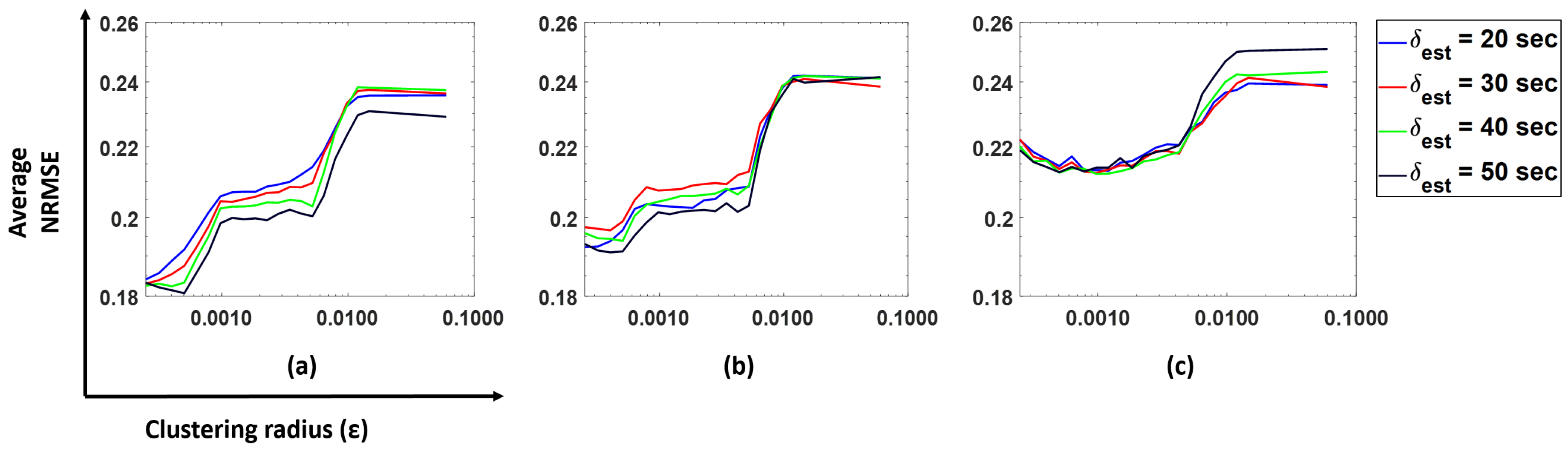
) chosen were 20, 30, 40 and 50 s. In
Figure 8, we plot the NRMSE (averaged over all subjects) as a function of
for the model predicting BR from HR using our cluster SVM strategy. Similar patterns were observed for other prediction models.
We observe that gives the lowest NRMSE for all forecast windows. Hence, we decided to choose s as our parameter for further analysis.
3.2. Cluster Analysis
We perform a hierarchical analysis on the clustering parameter to understand the effect of changes in the clustering as the
parameter increases.
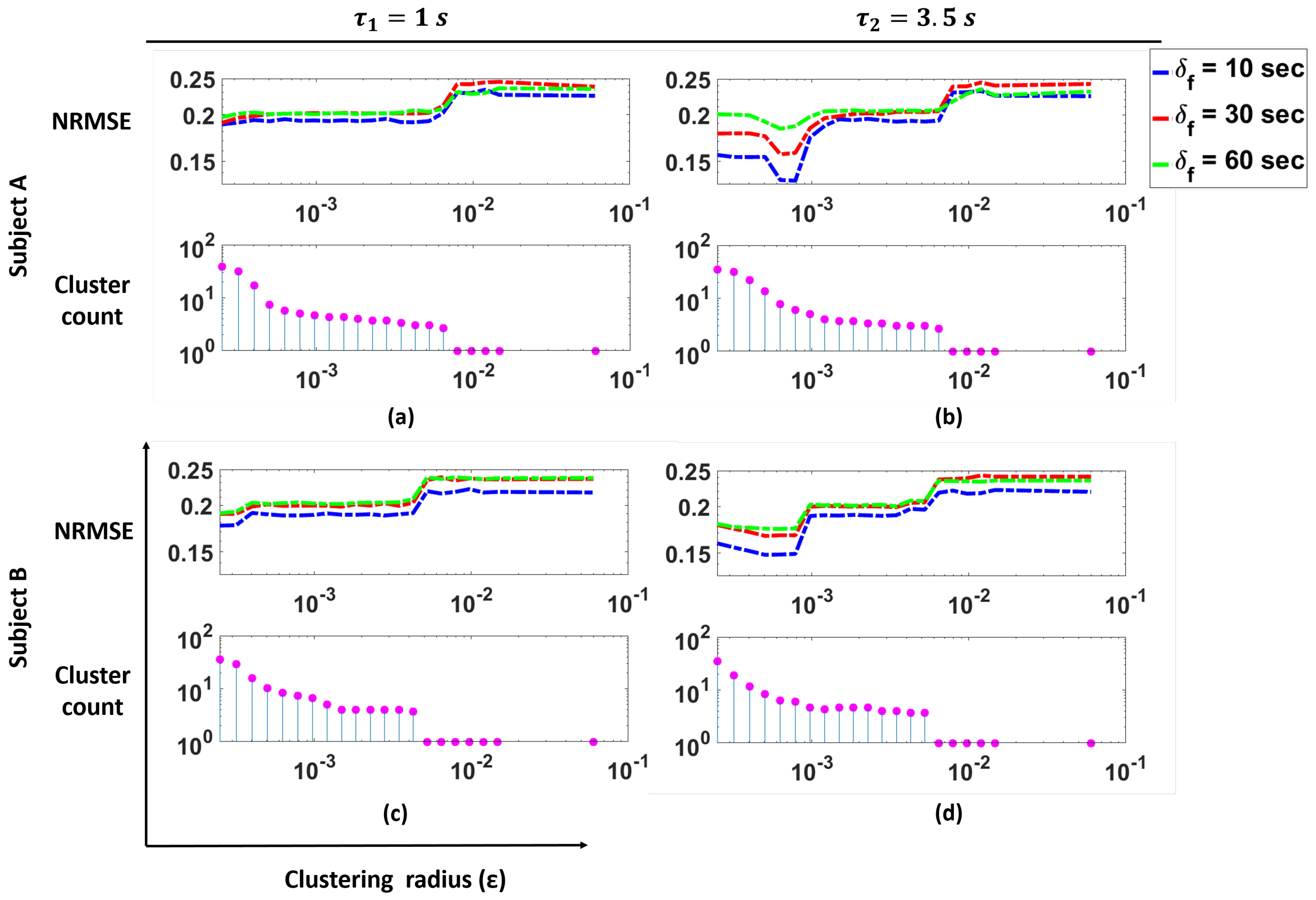
Figure 9 shows the NRMSE for the prediction of BR from HR using our cluster SVM strategy as a function of the clustering radius
for two subjects in the study, as well as the number of clusters as a function of
. These clusters correspond to the clusters remaining after outlier removal. In the figure, the plots for
s are shown.
These plots illustrate that for Subjects A and B, we see that changes in the cluster count have a significant effect on the NRMSE. Specifically, we see that smaller values of (i.e., more clusters are present) produce lower NRMSE. As the cluster count drops to one, we see a large increase in the NRMSE values. For both Subjects A and B, we see that with the appropriate number of clusters, a lower NRMSE can be achieved.
To further study the clustering outcomes, we analyze the correspondence between clusters and available activity labels from the dataset.
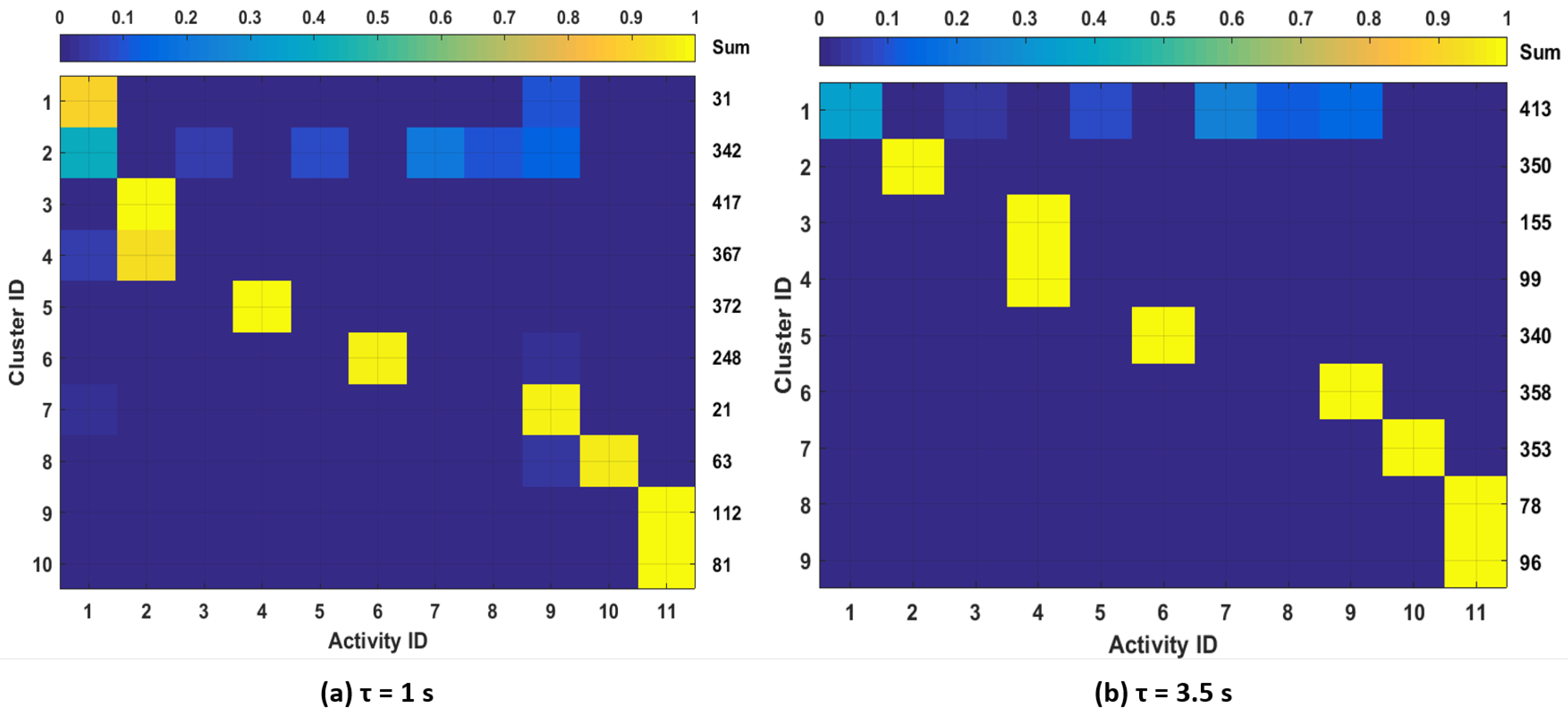
Figure 10 shows the distributions of data points in each cluster over the different activity labels for one subject. We show the results for
for which there is the largest number of clusters. In order to visualize the sample distributions in each cluster more clearly, we filtered out the clusters with less than 20 samples in
Figure 10. The total number of samples in each cluster is shown in the column labeled “Sum”. From the figure, we observe that different activities can be mostly associated with one or two clusters. We also observe that samples from activities: (3) “carrying a box,” (5) “drinking,” (7) “set dinner table” and (8) “clean up a table” were either merged with other activity clusters or filtered out. This is expected since these activities do not show motion patterns that are as distinctive as other activities such as running, rowing or bicycling. Considering these activities’ effect on physiological responses, it is reasonable to merge those activities with other low-intensity activities such as resting or walking and not train specific models since they are likely to have similar physiological responses.
3.3. Forecasting Breathing Rate
In this subsection, we perform prediction of breathing rate using our proposed approach. We analyze and compare predictions from
,
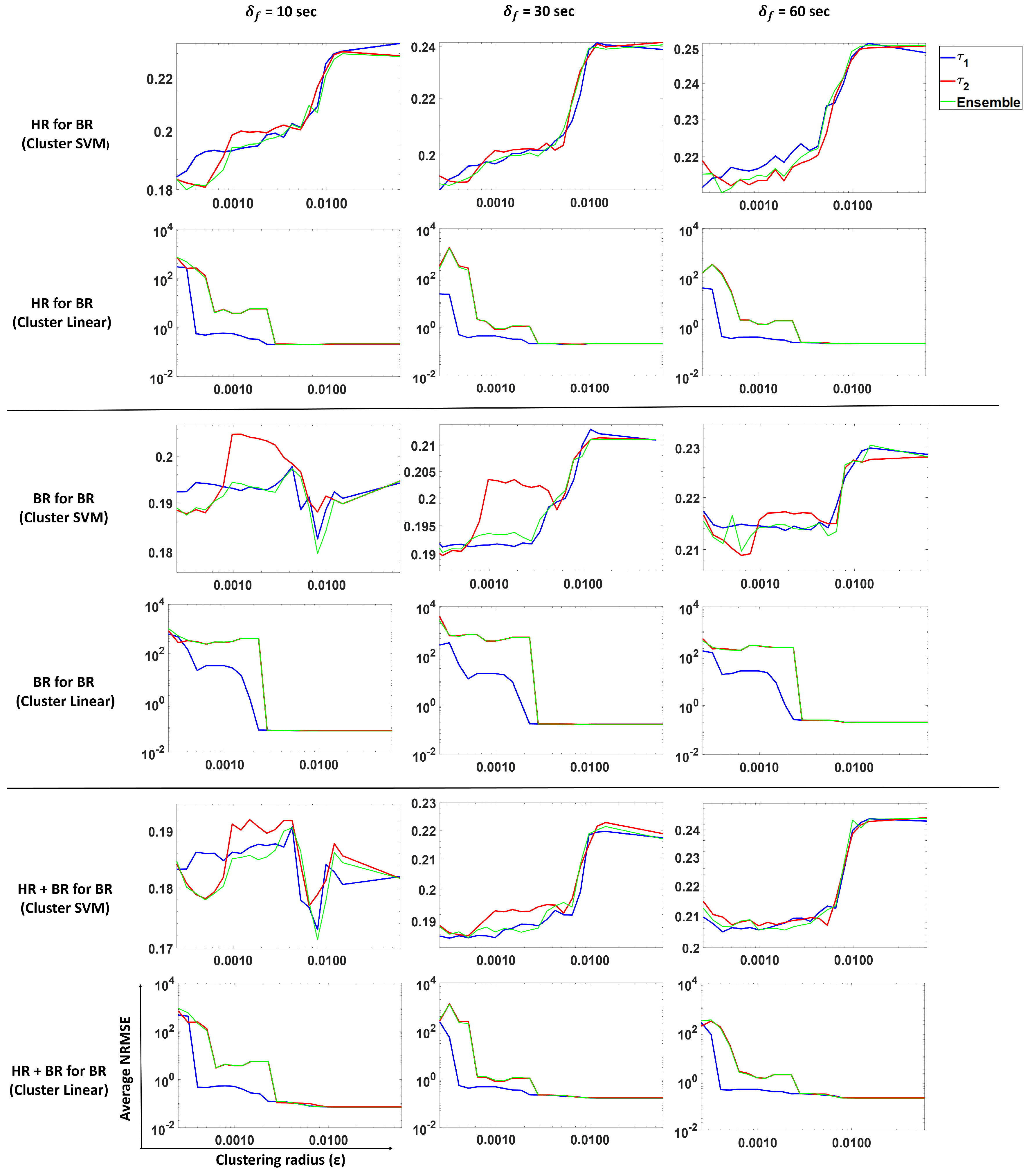
and ensemble methods. Models were trained for different scenarios: BR present, HR present and both BR and HR present. The results are shown in
Figure 11. Columns 1, 2 and 3 show average NRMSE values for a forecast of 10, 30 and 60 s, respectively, for
and ensemble predictions.
Each row in the figure depicts the following:
Prediction of BR with only HR (past) using an SVM regression (Gaussian kernel model).
Prediction of BR with only HR (past) using a linear model.
Prediction of BR with only BR (past) using an SVM regression (Gaussian kernel model).
Prediction of BR with only BR (past) using a linear model.
Prediction of BR with both BR and HR (past) using an SVM regression (Gaussian kernel model).
Prediction of BR with both BR and HR (past) using a linear model.
These results show (
Figure 11, Rows 1 and 2) that using heart rate can be useful to forecast breathing rate when the latter is not measured. In the SVM case (Row 1), smaller
values (more clusters) result in a lower NRMSE as compared to larger
value (fewer clusters). For
, we observe that the average NRMSE values increase dramatically as the number of clusters decreases (i.e.,
increases). However, the linear model (Row 2) does not show the same pattern, indicating that clustering does not help this model to predict BR from HR only.
The average standard deviation reported in
Table 1 corresponds to the average over all subjects of the standard deviation of all the predictions obtained per subject. Comparing the values from
Table 1, we see that clustering SVM performs best for a 10- and 30-s forecast, while for a 60-s forecast, the clustering linear and clustering SVM methods perform similar to each other. This indicates that for predicting BR from HR, clustering improves performance.
In the case where we predict BR with only past BR (Rows 3 and 4), the linear model and clustering linear perform the best, but give similar performance to each other. This indicates that a linear model is sufficient if historical values are observed when we are considering a short forecasting window. Clustering does not help in this scenario.
For the case of predicting BR with past HR and BR values (Rows 5 and 6), we observe that the linear model is sufficient to predict BR. Note that linear on around 10 clusters also shows a similar performance as the linear model on a single cluster. The differences between the values is not significant. From
Table 1, we observed that the models that use past BR perform just as well as the models that use past HR and BR values, which indicates that HR does not contribute much to the prediction when BR is present.
3.4. Forecasting Heart Rate
In this subsection, we perform the prediction of heart rate using our proposed approach. We analyze and compare predictions from
,
and ensemble methods.
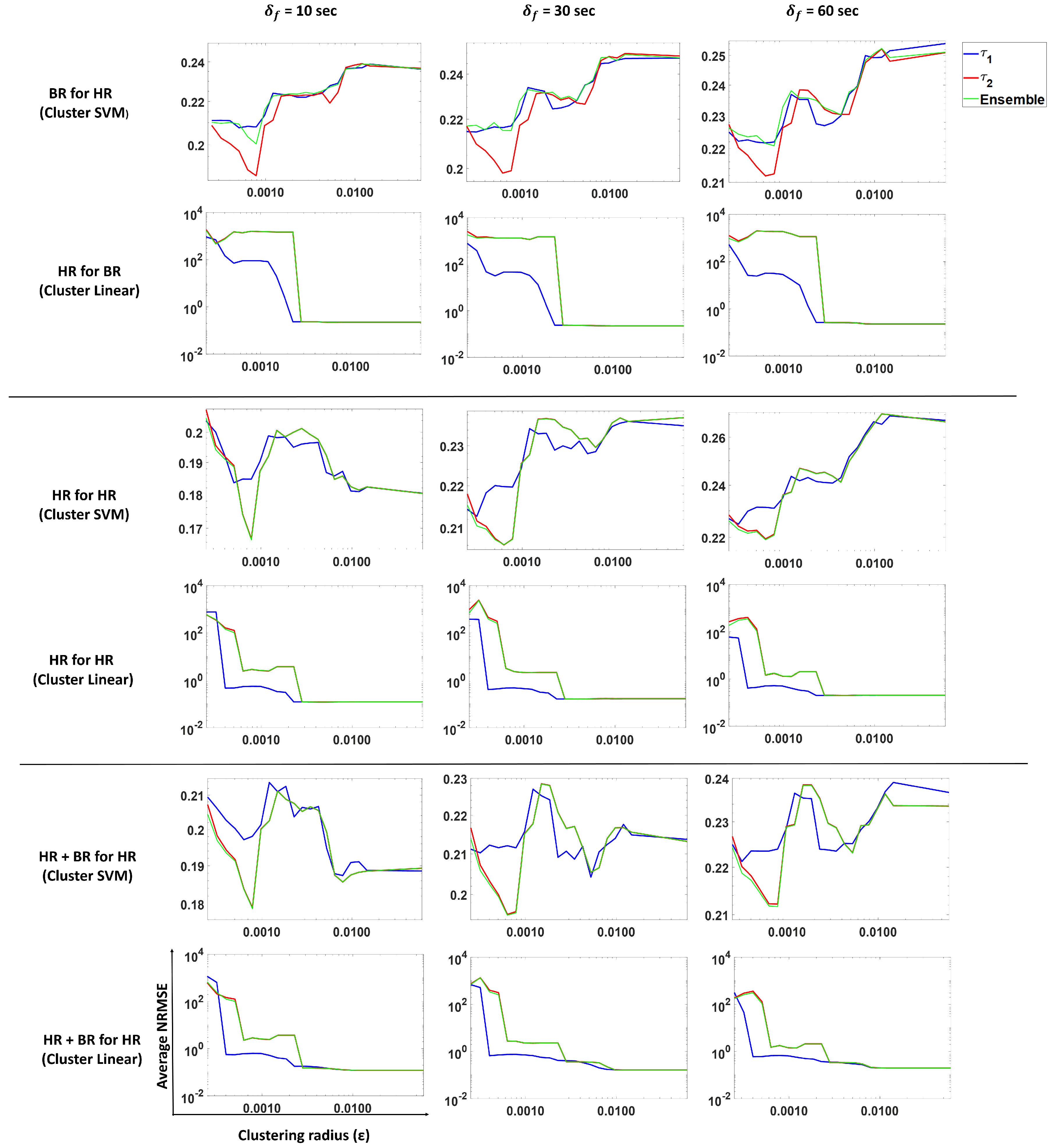
Figure 12 shows the results from three models trained for forecasting heart rate using SVM with the Gaussian kernel and the linear model.
Row 1 shows the NRMSE obtained by using an SVM regression (Gaussian kernel) on past HR for forecasting for , and the ensemble method. We see a similar pattern for 10-, 30- and 60-s forecasts. Smaller gives lower NRMSE values, while larger values result in larger NRMSE values. Similar patterns are observed for other models HR for HR and HR + BR for HR (Rows 3 and 5).
The average standard deviation reported in
Table 2 corresponds to the average over all subjects of the standard deviation of all the predictions obtained per subject. In the case of predicting HR with BR from
Table 2, we see that the clustering SVM performs the best for all forecast windows. This indicates that having clusters helps in this scenario.
In the case of predicting HR for HR, clustering linear performs the best for 10-, 30- and 60-s forecasts. Note that the linear model shows performance similar to the clustering linear model.
In the case of predicting HR using HR and BR, we see that a linear model is sufficient to predict HR. We also note a similar observation as in case of predicting HR for HR; the clustering linear and linear models show the same performance. From
Table 2, we observed that the models that use past HR perform just as well as the models that use past HR and BR values, which indicates that BR does not contribute much to the prediction when HR is present.
3.5. Comparison between Cluster-Aware Prediction and Traditional Modeling Methods
We compared our methodology to four state-of-the-art forecast/regression approaches: linear regression (LR), SVM regression with a Gaussian kernel (SVM) and random forest regression (RF). The train and test data was the same as used for our proposed approach.
Table 1 shows the prediction performance of each of these methods for forecasting windows
of 10, 30 and 60 s. Traditional modeling methods used in this setup are equivalent to having one cluster; a single model is trained over all the training data. For SVM regression with a Gaussian kernel, we choose the kernel scale heuristically. Random forests were trained for 50, 100, 150 and 200 trees in the model. We report the results for the random forest model that gave us the best performance (150 trees). All algorithms are implemented in MATLAB using the Econometrics Toolbox.
In
Table 1, we highlight the methods that gave us the best results (highlighted in blue). When it comes to forecasting BR just with HR measurements, the ensemble method with SVM regression is the best choice. These results are comparable to the errors seen when BR measurements are available. This is a strong indicator that HR can be used to forecast BR within the experimental setup under consideration.
In the case of forecasting BR with past BR, we expect BR to be linearly related to past BR, i.e., the linear model should perform better in this case.
Table 1 (column for “BR for BR”) shows that for 10-, 30- and 60-s forecasts, the cluster linear model and linear model perform the best with a small difference between them.
Using both HR and BR to forecast BR, we see that the linear regression without clustering performs better for all forecast windows. We observe that the terms associated with HR are not significant (large p-values); only past BR values are dominant in the prediction. Hence, we see similar results as for the case when we predict BR with past BR values only.
In terms of forecasting HR, we note the following observations from
Table 2. Forecasting HR with past BR shows the same pattern as in the case of forecasting BR with past HR. Cluster SVM gives the lowest NRMSE for all forecast windows. We note that in cases of cross-modality forecasts, a non-linear model captures the non-linearity in the relationship between HR and BR and that clustering helps in this scenario.
Forecasting HR with past HR values also shows similar results as in the case of forecasting BR with past BR. Finally, using past BR and HR to forecast HR, we see that the linear and cluster linear methods are interchangeable, giving the lowest NRMSE, with a slight difference in the values. The models yield values similar to the one returned by the model where we use past HR to forecast HR. This along with the coefficient analysis indicates that the past BR values are not contributing to the model.
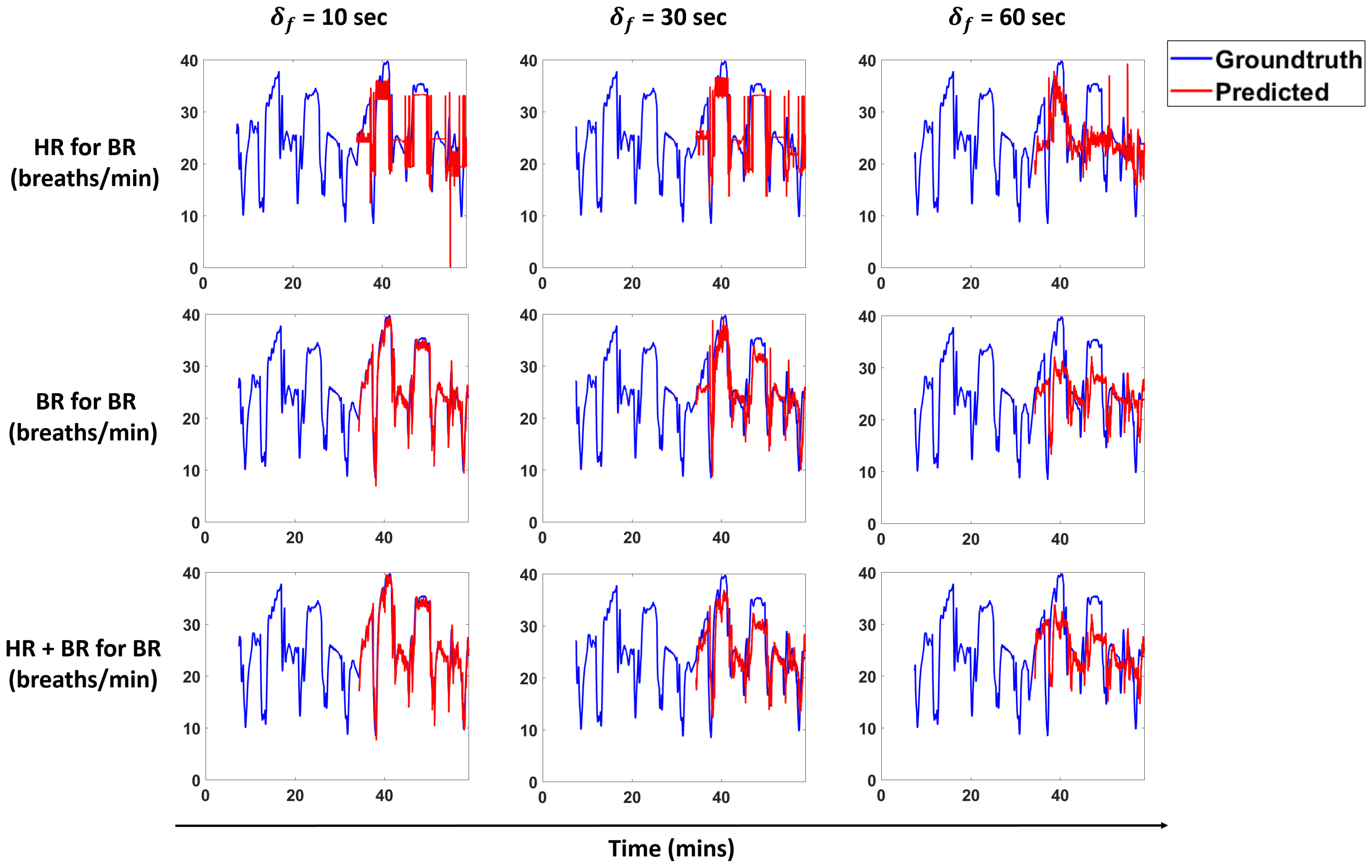
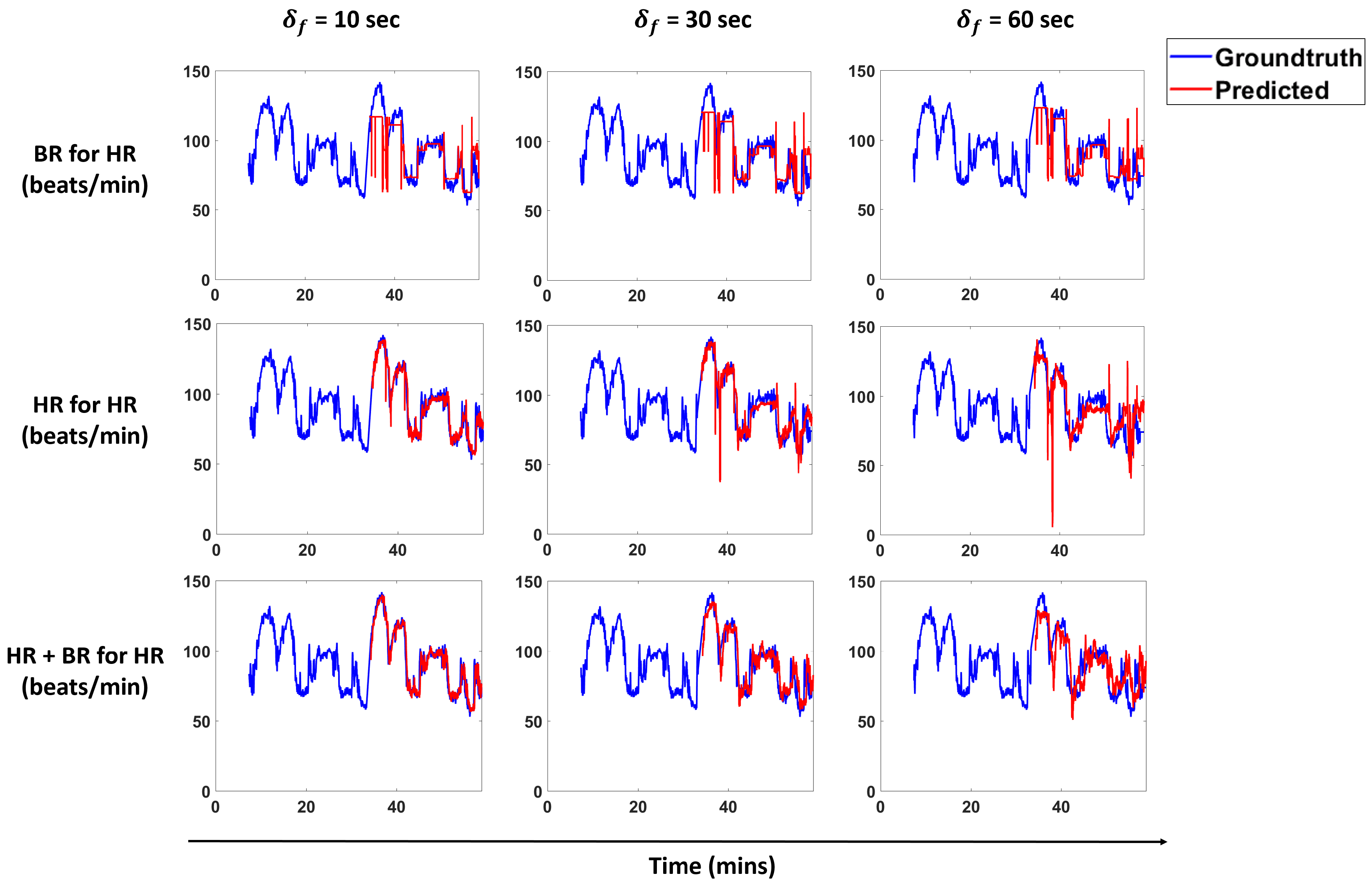
Figure 13 and
Figure 14 show predictions for a subject for the models that perform best for each scenario. We overlay the forecasts with the ground truth.
4. Conclusions
We propose a pipeline to forecast physiological parameters consisting of models based on an unsupervised physical activity clustering. Forecast results for a subject are shown in
Figure 13 and
Figure 14. We experimented with different types of models to study the relationship between the physiological quantities and physical activities. Detailed experiments were also conducted to study the effects of different window sizes and clustering radius in the pipeline.
We demonstrate that clustering based on activities and only using past heart rate (HR) values is sufficient to forecast breathing rate (BR) in our experimental setting. The results for this scenario are comparable to forecasting BR just with the history of BR, thus indicating that HR in conjunction with activity clusters is a good predictor and can help in cases when we do not have BR measurements. A similar trend is seen for the scenarios of predicting HR with BR and activity clusters.
Results show that clustering does not help much in cases where we forecast BR with past BR values and HR with past HR values. For both of these scenarios, we see that the linear model and cluster linear model perform similar to each other. This is true for the case when we predict BR with past BR and HR values and HR with past BR and HR values. All of these scenarios indicate that a linear model is sufficient for these cases. In cases where the prediction is across modalities (i.e., HR for BR and BR for HR), we conclude that clustering is beneficial to get a lower NRMSE as compared to the non-clustering methods.
We aim to extend this work in a number of ways in order to design more accurate models that incorporate environmental factors, as well as cognitive and affective states [
46]. From an environmental perspective, we will aim to add sensing modalities that capture temperature, humidity, concentrations of particulate matter, etc. In order to capture affective state information, we can make use of sensors such as galvanic skin response (GSR) sensor, which are known to be correlated with arousal [
47]. Furthermore, more contextual information can be utilized, as well, by providing location information (e.g., GPS) or surrounding noise-levels. For these extensions, the outcomes of this study can serve as a guideline for the use of appropriate predictive models and provide a baseline for the levels of accuracy that should be expected.


