An Automated Technique for Extracting Phasors from Protective Relay’s Event Reports
by
 , , and
Sundaravaradan Navalpakkam Ananthan
1,* ,
,
Alvaro Furlani Bastos
1,
Surya Santoso
1 and
Alberto Del Rosso
2 1
Department of Electrical and Computer Engineering, The University of Texas at Austin, Austin, TX 78712, USA
2
Electric Power Research Institute, Knoxville, TN 37932, USA
*
Author to whom correspondence should be addressed.
Inventions 2018, 3(4), 81; https://doi.org/10.3390/inventions3040081
Submission received: 15 November 2018
/
Revised: 9 December 2018
/
Accepted: 10 December 2018
/
Published: 13 December 2018
(This article belongs to the Special Issue Emerging Technologies Enabling Smart Grid)
Abstract
:Post-fault event report analysis is a crucial skill set for electric power engineers in the protection industry. This paper serves as a reference which elucidates the preprocessing procedures involved in transforming data present in event reports to phasors that can be used in various post-fault analysis application algorithms. The paper discusses key elements of this process such as interpreting the data and calculating voltage and current phasors from instantaneous sample values present in a fault record. A crucial component of event report analysis is choosing the appropriate time instant for calculating phasors for event report analysis. Conventionally, protection engineers manually perform event report analysis and arbitrarily select time instants after certain cycles of fault inception for this purpose. This approach prevents the process from being successfully automated. Furthermore, arbitrary selection of time instant does not utilize the entire fault data and may fail in several cases such as short time fault scenario and evolving fault scenario. For this purpose, this paper proposes an adaptive novel technique which utilizes the entire data present in the event report to select the most suitable time instant for event report analysis. The superiority of the proposed algorithm over conventional methods is demonstrated using three real-world scenarios.
1. Introduction
Transmission lines are a vital part of a power system as they transfer electrical power over long distances from generators to loads. Transmission lines are usually uninsulated and are subjected to a variety of faults. When a fault occurs in a power system, voltage and current waveforms are recorded by intelligent electronic devices (IEDs) such as digital relays and digital fault recorders (DFRs). Event reports recorded during a fault contain a plethora of information about the system condition [1]. Event reports have been traditionally used for performing fault analysis such as identifying the fault location [2,3,4,5] and fault resistance [6]. In recent times, they have been used for a variety of purposes such as evaluating relay and circuit breaker performance [7,8,9] and gleaning system parameters such as sequence impedance parameters of lines [10,11,12], estimating Thevenin impedance [13], verifying short circuit system model used for studies [14], and determining the exact fault inception and clearing times [15,16].
Different digital fault recorders have different recording capabilities and specifications. Fault recorders capture instantaneous snapshots of the various quantities it measures and records it in the event reports. Hence, these data present in the form of samples need to be preprocessed to extract information in a usable format for implementing the various event report analysis applications discussed previously. Past efforts in developing event report analysis applications commonly either use data obtained from simulation results or directly use phasors obtained from real-world data for demonstrating their applications. When simulation results are used, the data are readily available in the required format. Hence, either way the preprocessing steps are neglected.
In the data preprocessing stages, though the process of obtaining phasors from data present in the form of discrete samples is fairly a simple process, there exist a crucial step which is choosing the time instant for extracting phasors which would then be used in the event report analysis application algorithms. Historically, an arbitrary time instant after fault inception has been chosen to extract phasors for this purpose. A major cause of transients in the fault current is DC Offset and phasor estimation performed while DC offset is present, which can lead to errors in analysis applications [17,18]. DC offset is commonly expected to drown out within a few cycles [19]. Hence, phasors 2 cycles after fault inception are extracted for this purpose. However, this selection process is further complicated when there is CT saturation present due to DC offset. Asymmetrical CT saturation can take several cycles to occur [20]. Authors in [21] have used 1.5 cycles after fault inception as their time instant for extracting phasors. The authors in [10] have identified other factors apart form CT saturation such as capacitive voltage transformer (CVT) transients which can last for about 1.5 cycles. Selecting phasors just 1.5 cycles after fault inception may be too quick as the transients may not have died out within this period in real-world cases. Some authors have taken a more conservative approach and used 3 cycles after fault inception as the point for estimating phasors for this purpose [11,12]. A most likely scenario where this choice of time instant will fail is when the fault has been cleared very quickly and as a result, the fault segment is not long enough. The authors from practical experience have clearly pointed out in [22] some of the sources of error which can arise from event report analysis of transmission line faults. In the very first case analyzed in [22], the relay calculated an inaccurate fault location estimate because it could not choose the appropriate phasors during an evolving fault. The algorithm used in that scenario assumed that the contiguous data midpoint is a reasonably stable point at which to estimate the fault location. The authors have highlighted the issue of choosing the best point in the event report for fault location estimation. Furthermore, there are several research papers and reports which have also emphasized the need to select appropriate time instants for extracting phasors for various applications. For example, [3,23] have stressed on the importance of choosing the best part of the fault waveform for extracting phasors to be used for fault location in transmission and distribution systems. Studies performed in [24] have identified inaccurate phasor selection due to various factors as discussed previously as a source of error while estimating fault location in transmission systems.
The commonly used time instants have been 1.5, 2, or 3 cycles after fault inception for extracting phasors for event report analysis applications. Furthermore, many of these applications have been calculated off line. If these commonly chosen time instants are not used, they are chosen by visual inspection by protection engineers. However, like fault location, several of these applications such as estimating sequence impedance parameters of the line and relay performance verification can be automatically calculated every time a fault event report is recorded and used as a supervisory check of system condition. This would be possible if we can identify the appropriate phasors to be used for calculations accurately so as to not raise any false alarms.
Summarizing this, different authors have used a variety of time instants for extracting phasors to be used in event report analysis applications. When fault instants are chosen arbitrarily, there is no confidence or guarantee that steady state has been achieved at the selected time instant. Furthermore, the fault record may contain longer periods of steady state fault data which offer better quality of information but would not be utilized when a fixed arbitrary time instant is chosen for all cases. It is common sense to use data after the transients have died out for this purpose. However, there has not been a technique to identify this time instant from a steady state fault portion of the event report. Moreover, in the modern world where several functions are being automated, there needs to be a way to quantify steady state so that the digital relays or processors themselves can accurately calculate and perform event report analysis applications. A proposed method for estimating the time instant should also be simple enough to be comprehended by the relay engineer, who should be able to verify and rectify the results in abnormal situations.
This paper presents a novel method to identify a time instant from the steady state portion of an event report for the extraction of phasors for event report analysis applications. This paper also serves as a tutorial and elucidates the data preprocessing steps required to be performed to transform data present in event reports into phasors that can be used in various algorithms as discussed in Section 2. The proposed novel method to select phasors for event report analysis applications is presented in Section 2.2. Section 3 demonstrates the effectiveness of the proposed algorithm in event reports that have transients such as DC offset, short time fault scenario, and evolving fault scenario using field data obtained from three real-world cases. The time instant chosen by the proposed algorithm is compared with commonly used time instants of 1.5, 2, or 3 cycles after fault inception for extracting phasors for event report analysis applications. The proposed algorithm generalized well for all the presented fault scenarios and chose appropriate time instant for extracting phasors from event reports, thus eliminating errors in post-fault analysis application due to wrong selection of phasors.
2. Methodology for Data Preprocessing
Recording devices are primarily used to monitor and record voltages, currents, and status signals when triggered due to certain events. Recording devices may differ in sampling rate, length of record, and type of record they can capture based on their purpose of usage [25]. Some of the common types of recording devices are microprocessor-based relays and digital fault recorders.
When recording devices detect any disturbances or faults, they are configured to produce fault records such that they contain prefault information, event or fault data, and post-fault information. The recording device can be triggered by a variety of conditions such as over-current, change in observed voltage, frequency, or impedance based on its setting. Prefault data contains information regarding the normal system conditions just before the fault or disturbance occurs. Event data contains fault voltages, currents, and status of protective devices and switchgear (if monitored by the recorder). Post-fault information shows how the system has responded and operated under the fault condition.
Though the data preprocessing step has been automated inside the relay for certain applications, some applications still require a protection engineer to manually perform this process to extract different quantities from event report for analysis. The following sections will explain the steps which need to be performed to transform raw data into useful phasor quantities that can be used in various algorithms.
2.1. Obtaining Fundamental Frequency Phasors
The measurements obtained from fault records are discrete samples. There are several methods that have been proposed over the years such as discrete Fourier transform (DFT), cosine filters, least squares algorithm, Kalman filters, and wavelet transforms to filter out certain quantities such as harmonics or DC offset [26]. In this paper, discrete Fourier transform is used for calculating the phasors. DFT technique can efficiently extract the magnitude and phase angle of only the fundamental frequency voltage and current and discard all the harmonics. On applying DFT, we extract the peak value magnitude and phase angle of the fundamental frequency. This magnitude is then divided by to obtain the RMS value.
DFT is applied on one cycle data. The number of samples present in one cycle depends on the sampling frequency of the recorder. The current and voltage frequency (f defined in hertz), sampling rate ( defined in samples per cycle), and the total number of samples present (n) are usually saved in the fault record as supplemental information. A sliding window of size of one cycle (or size samples) is used where the oldest sample is discarded when a new sample is added.
One of the ways of applying DFT over the entire sample set is by using each sample in the fault record as the last sample in the DFT calculation as shown in Figure 1. Hence, each sample at index p in the set will have a corresponding fundamental phasor quantity (at index p) which will also be the RMS value. The set containing all the current magnitudes is called and the set containing all the voltage magnitudes is called . The calculation of phasors is done for the entire fault record to be able to visualize the current and voltage magnitudes during the fault as well as to identify an appropriate fault instant and prefault instant to extract phasors for event report analysis.
2.2. Algorithm to Select Phasors for Event Report Analysis Applications
Most event report analysis applications such as calculating fault location, estimating sequence-impedance parameters, and Thevenin impedance of upstream network require a stable prefault and fault instant values of voltage and current phasors. Though selection of prefault quantities is a straightforward process, the selection of fault quantities is more complicated as discussed in Section 1. This subsection proposes an algorithm which can select an appropriate time instant for extracting phasors during a fault which can be used for event report analysis applications.
Event recorders record certain number of cycles before the actual trigger which caused them to save an event report. These cycles of data are called prefault data. In most scenarios, except energizing events and recloser operation events, before a fault has occurred, the voltage and current values are stable in all three phases. Hence, it is simple to pick a prefault instant. The prefault time instant can be any sample before the onset of the fault. A commonly selected time instant for obtaining prefault quantities is 3 cycles before the inception of the fault. The current at the prefault instant and the fault instant is denoted by and respectively in this paper. However, to avoid any phase angle mismatch between the prefault and fault phasors, the difference in the number of samples between the fault instant and prefault instant at which the respective phasors were calculated must be an integer multiple of the sampling rate as shown in (1). Once the fault instant for extracting phasors for analysis applications is chosen, the prefault instant can be modified accordingly.
Conventionally, arbitrarily chosen time instants after fault inception are used to extract phasors for analysis. These values are fixed values and are not adaptive based on the fault waveform. Hence, there is a need to have an adaptive method which is also comprehensible by protection engineers that analyzes the entire fault waveform to identify an appropriate fault instant to extract phasors for event report analysis applications.
The proposed algorithm for selecting the fault instant is presented in Figure 2. After calculating the RMS current and voltage magnitudes over the entire fault report as shown in the previous subsection, the next step is to identify the portion of the event report which contains the fault. In most scenarios, the fault current is a minimum of three to five times the prefault current. This parameter is commonly used to detect the fault inception [27]. In this algorithm, when the current magnitude at index p is greater than three times the prefault current magnitude, it is identified as part of the fault. The set containing all such time instants is called the faulted cycles (FC) and is defined according to (2).
The aim is to find a stable time instant to obtain the current and voltage phasors. This means that the variation in current and voltage magnitude must be minimal surrounding this time instant to certify that steady state has been reached at the selected time instant.
A sliding window of size is defined for this purpose. The sliding window at index p contains magnitude values at indices ranging from to . The moving window is given by (3) and is elucidated in Figure 3.
where . The indices and denote the time corresponding to the first and last elements of the faulted cycles set (FC) respectively.
This window at index p includes a quarter cycle equivalent of current magnitudes prior to instant p and quarter cycle equivalent of current magnitudes past instant p. Calculating the variance of values inside this window will reflect on the variation of current or voltage magnitude of nearly one and half cycles. It is to be remembered that each magnitude value is calculated by using one cycle of samples in DFT. Hence, the size of the set and are . The variance of the elements in the sliding window is calculated using (4). The sliding window is applied from index to of the FC as this represents the fault portion of the event report for both current and voltage magnitude.
The variance of N elements present in a data set vector A with a mean of is defined using
The set of variance values obtained by moving the sliding window over the current magnitude is rescaled to the range of . Rescaling the elements present in a data set vector is done using
where and are the smallest and the largest elements in respectively.
Similarly, the set of variance values obtained by moving the sliding window over the voltage magnitude is rescaled as well. The rate at which voltage changes is proportional to the rate at which current changes as they are related together by the impedance of the system (Ohms law). As a result the shape of current and voltage variance graph is expected to be similar. This allows us to rescale the variance in voltage values and rescale the variance in current values as well.
The calculated rescaled current variance at index is summed with the calculated rescaled voltage magnitude variance at index for each index between and . The index with the minimum value of summed variance quantities () is chosen as the time instant which has the most stable current and voltage values that is most suitable for event report analysis applications. The corresponding starting current or voltage sample number to calculate phasors is called . The pseudocode for the proposed algorithm is presented in Figure 4. By implementing this algorithm, we are effectively identifying stable or least varying voltage and current values over a period of one and a half cycles. A small variance value during the faulted segment of the waveforms represents that the fault has reached steady state conditions. When the variance is large, the samples probably correspond to the transition segment and is yet to reach steady state fault condition.
Statistical hypothesis testing methods such as two sample t-test for testing mean equality and F-test for testing variance equality using and or corresponding voltage quantities as two sets of data as proposed in [28], cannot be performed because the sets of data used for analysis must correspond to a normal distribution. This assumption that portions of the rms current and rms voltage profiles will belong to a normal distribution cannot be made, especially during a fault event where there are step changes in the values. Furthermore, two sample t-test and the F-test would be a much stricter test to check for steady state conditions and cannot be implemented in short time fault events where steady state may not be reached at all.
Different recording devices record event reports at different sampling rates (). When the sampling rate changes, the change in voltage or current magnitude between successive samples vary. Hence, a method which uses a threshold value to identify changes or rate of change or lack of variation in voltage and current magnitude between successive samples to detect steady state condition cannot be used. The proposed algorithm is not affected by changes in sampling rate because the number of samples within the sliding window in (3) changes based on the sampling frequency. As a result, it will capture the variations in current and voltages over a period of 1.5 cycles, irrespective of the sampling frequency.
3. Validation of Proposed Algorithm Using Field Data
As seen in Section 1, different authors have used a variety of instants and some of the commonly used values are 1.5, 2, or 3 cycles after the fault inception to obtain stable fault phasors for event report analysis applications. This section compares these different time instants with that of the proposed method to demonstrate the advantages and efficacy of the proposed method.
For this purpose, 3 event reports obtained from actual real-world fault scenario are analyzed. In each of the event reports, the fault instant selected by the proposed algorithm is validated by estimating the fault location and comparing it with actual fault location identified by the electric utility. Single ended impedance-based fault location methods have been used here because they utilize known system parameters and fundamental frequency fault voltage and current measurements obtained from event report [3,19]. The calculated fault location would be much different from the actual fault location if the current and voltage phasors at the selected time instant contains transients and DC offset. Furthermore, the fault instant selected by the proposed algorithm is compared with other arbitrarily chosen fault instants discussed previously. Different fault location algorithms have different input requirements. Hence, the purpose of providing fault location with different algorithms is to show and verify that the time instant chosen by the proposed algorithm is a good point for selecting phasors to be used as inputs for performing any variety of event report analysis application requiring different input data from event reports, and not for comparison of fault location obtained between different algorithms.
3.1. Case 1: A Common Fault Scenario
The first case taken for analysis is a line-line fault involving B and C phases. The faulted line is a 138 kV, 12.88-mile long line. The breakers protecting the circuit tripped and locked out because a tree fell on the line about 2.64 miles from substation.
Figure 5 shows the current and voltage waveforms related to the faulted line present in the fault record showing the first trip operation. The sampling frequency of the fault record was 3840 Hz or 64 samples/cycle. The swell in the current waveforms in phases B and C clearly indicate the presence of a line-to-line fault.
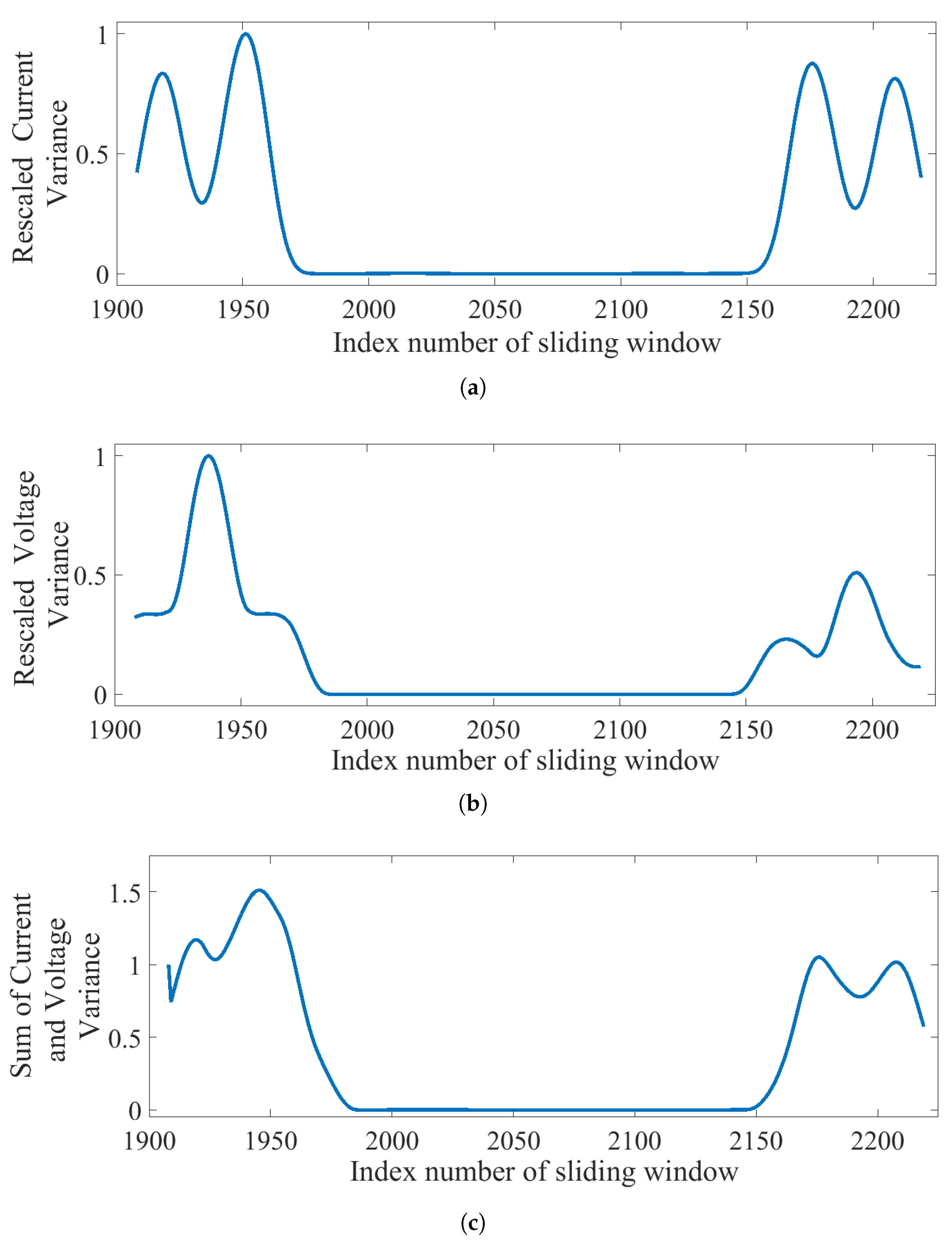
From Figure 6 and by calculating the FC set, the fault inception was calculated to be at sample number 1908. The markers on the current and voltage profiles (Figure 6) correspond to the time instants presented in the Table 1. The first two diagrams in Figure 7 shows the calculated rescaled variance values of current and voltage magnitudes at each sliding window index respectively. The third diagram in Figure 7 shows the summed up value of rescaled current and voltage variance at each index . The time instant corresponding to the index number which has the lowest value in this summed up variance plot is chosen as the stable point for event report analysis applications. It is possible to visually verify from the voltage and current profiles shown in Figure 6 that the current and voltage magnitudes have reached steady state at the instant selected using the proposed algorithm. This time instant () has been shown using a red cross in Figure 6.
As this scenario is a simple common scenario without complications, choosing an arbitrary time instant of 1.5, 2, or 3 cycles from fault inception seems to have provided us with reasonable fault location estimates. The proposed algorithm too has chosen a time instant that has reached steady state. However, it can be observed in Case 2 and Case 3 that the time instant selected by the proposed algorithm has minimal current and voltage variations in the time period surrounding it compared to some of these arbitrarily selected time instants.
Table 1 presents the sample number index corresponding to the number of cycles past the fault inception. It also gives the fault location calculated using phasors extracted at that time using DFT as explained in Section 2.1. It can be seen that the proposed method chooses a time instant where the fault current and voltage waveform have been steady for one and a half cycles around the selected time instant.
3.2. Case 2: A Short Time Fault Scenario
The second case chosen for analysis is a transmission line fault on a 345 kV line which is 69.94 miles long. The event files from the monitoring station revealed that there was a single line-to-ground fault on the line creating around 6 kA of fault current on B phase of the line. Protection engineers had identified that the fault was at 15.33 miles from the monitoring station caused by buzzard droppings on the insulator.
The relevant waveforms of the faulted line present in the fault record are shown in Figure 8. The sampling frequency of the fault record was 960 Hz or 16 samples/cycle. Phase B current waveform clearly shows an increase in magnitude while phase B voltage waveform shows a sag which is indicative of a single line-to-ground fault on phase B.
From the waveforms in Figure 8 and the voltage and current profiles in Figure 9, it can be observed that the fault existed for a very short time interval but it reached steady state within this time period.
It can be seen from Figure 9 and Table 2 that the third cycle after fault inception is not available. When the time instant two cycles after fault inception is chosen, it is too late as the process of fault clearing has already begun. This is reflected in current and voltage profiles as well as in the estimated fault location. Choosing 1.5 cycles provided reasonable results in this case but choosing 1.5 cycles after fault inception as a default value might be too early for many other fault scenarios as the transients may not have died down within that time period.
The proposed method chose an appropriate time instant according to the fault data without waiting for minimum arbitrary time period. The steady state condition was reached much before 1.5 cycles after fault inception. The proposed algorithm was able to detect this by using the variance parameter and pick a time instant from the steady state condition.
3.3. Case 3: An Evolving Fault Scenario
This case presents an evolving fault where the fault started as a single line-to-ground fault on C phase (CG fault) but then evolved into a line-to-line-to-ground fault involving A and C phase (CAG fault). The fault in A phase was temporary and cleared out in a few cycles, however, the fault on C phase was a permanent fault. The fault was identified to be caused due to lightning on a line of length 4.84 miles. The fault location identified by the utility was 2.67 miles from the measuring location.
The recorded fault waveforms for this case are shown in Figure 10. The sampling frequency of the fault record was 1920 Hz or 32 samples/cycle.
This scenario will demonstrate that irrespective of how the fault is classified by the relay, the algorithm will provide appropriate time instants corresponding to the type of fault identified for extracting phasors to be able to successfully perform event report analysis. This would not be possible if arbitrary time instants after fault detection are chosen for extraction of fault phasors.
3.3.1. Fault Detected as an CG Fault
Though the expected fault detection is CAG fault, it is possible that the relay might classify it as a CG fault because the fault started as a CG fault and existed as a CG fault for several cycles. When the event report is analyzed as a CG fault, we focus only on the current and voltage waveforms of C phase for our analysis.
Table 3 shows the sample numbers at different time instants after fault inception. Figure 11 shows the current and voltage magnitudes when analyzing the fault as a CG fault. In contrast to case 2, at 1.5 cycles after fault inception, it can be observed that the current and voltage profiles have not settled yet from their DC offset. Any point before the fault evolved into CAG fault, such as two or three cycles after fault inception, would lead to incorrect values because of transients caused by the evolution of the fault. The current and voltage waveforms are not stable until the fault has developed into CAG fault and this can be observed in the profiles shown in Figure 11 as well. Hence, a good algorithm is expected to pick a value after the fault has grown into CAG fault.
If a fault instant is picked to be at the middle point of the faulted portion of the waveform according to the method used in [22], it would have chosen a value in the midst of the CAG fault (around 259) which may have resulted in an erroneous reading. The fault may still be evolving and there is no guarantee that the fault has reached steady state at this time.
It can be seen from profiles shown in Figure 11 that the current and voltage waveforms have not reached steady state and are still fluctuating at times instants 1.5, 2, and 3 cycles after fault inception. This is reflected in Table 3 as well because the estimated fault location keeps changing at these time instants. The proposed method, on the other hand, was able to choose a time instant after the fault had reached steady state. This is also visually clearly perceptible from the current and voltage profiles and the estimated fault location is closer to actual fault location at this time instant in comparison to the other commonly chosen time instants.
3.3.2. Fault Detected as a CAG Fault
When the fault is classified as a CAG fault, the fault exists as a CAG fault only for a few cycles as seen in Figure 12. Hence, this rules out the possibility of selecting a time instant in terms of cycles after fault inception. Similar to case 2, the fault does not exist at three cycles after the fault starts evolving into CAG fault. However, arbitrarily selecting 1.5 or 2 cycles after fault inception may work for this case (as seen from the fault location estimates presented in Table 4) but there is no assurance that it is the most steady time instant to obtain the phasors for event report analysis. On the other hand, the proposed algorithm analyzes the entire waveform where CAG fault exists and provides the time instant with the least current and voltage variation, hence ensuring that the best available current and voltage phasors are chosen for event report analysis.
3.4. Discussion
In the scenarios shown above, there may not be an improvement in fault location accuracy between some of the arbitrarily chosen time instant and the time instant calculated by the proposed method because there are several sources of errors while implementing impedance based fault location methods [19]. It has also been shown that no single arbitrarily chosen time instant worked for all the cases shown above. However, by using points selected by the proposed method, it can be guaranteed that errors due to wrong selection of phasors such as that reported in [22] can be eliminated, i.e., the proposed algorithm generalized well for all fault events. The algorithm is resilient and not affected by the sampling frequency of the event report and has proved to be robust to different types of fault scenarios, such as short time faults and evolving faults, as shown in this section.
This algorithm enables several post-fault analysis applications to be automated with high level of reliability. Presently, protection engineers skillful in electrical engineering concepts manually perform event report analysis and supervise automated control systems. However, they may not be familiar with advanced mathematics. This algorithm is intuitive to understand for protection engineers and does not involve unnecessary complex transformations.
4. Conclusions
This paper proposes an algorithm to select an appropriate time instant in a fault record to extract phasors that can be used for event report analysis applications. Conventional methods use arbitrarily chosen time instants after the fault inception which may not be suitable for all scenarios. They also do not explore and make use of the entire fault data which may provide better quality of information. On the other hand, the proposed method is adaptive in nature and uses statistical tools to select a time instant where the fault current and voltages are stable and suitable for post-fault analysis applications. This paper demonstrates the proposed algorithm using three real-world test cases. The benefits and superiority of the proposed algorithm are highlighted in this paper using a short time fault scenario and an evolving fault scenario.
This paper also serves as a reference elucidating the preprocessing procedures involved in transforming data present in event reports to phasors that can be used in various post-fault analysis application algorithms. This paper sheds light on every step starting from interpreting data present in fault records, calculating voltage and current phasors from instantaneous sample values recorded by a digital fault recorder, and selecting the appropriate phasors for event report analysis application. This paper will enable a protection engineer with all tools required to perform post-fault analysis using fault records.
Author Contributions
The conceptualization, development of the algorithm, analysis and writing the manuscript was done by S.N.A. A.F.B. assisted with reviewing and editing the manuscript. S.S. was the advisor mentoring the project. A.D.R. provided the resources for demonstration of the algorithm.
Funding
This research received no external funding.
Conflicts of Interest
The authors declare no conflict of interest.
Abbreviations
The following abbreviations are used in this manuscript:
| IED | Intelligent Electronic Devices |
| DFT | Discrete Fourier Transform |
| RMS | Root Mean Square |
References
- Costello, D. Understanding and analyzing event report information. In Proceedings of the 55th Annual Georgia Tech Protective Relaying Conference, Atlanta, GA, USA, 2–5 May 2001; pp. 1–52. [Google Scholar]
- Schweitzer, E.O., III. A review of impedance-based fault locating experience. In Proceedings of the 14th Annual Iowa-Nebraska System Protection Seminar, Omaha, NE, USA, 16 October 1990. [Google Scholar]
- IEEE. IEEE Guide for Determining Fault Location on AC Transmission and Distribution Lines; IEEE Std C37.114-2014 (Revision of IEEE Std C37.114-2004); IEEE: Piscataway, NJ, USA, 2015; pp. 1–76. [Google Scholar]
- Ananthan, S.N.; Santoso, S. Universal model-based fault location for improved system integrity. IET Gener. Transm. Distrib. 2018. [Google Scholar] [CrossRef]
- Saha, M.M.; Izykowski, J.J.; Rosolowski, E. Fault Location on Power Networks, 1st ed.; Springer: London, UK, 2010. [Google Scholar]
- Xia, B.; Wang, Y.; Vázquez, E.; Xu, W.; Wong, D.; Tong, M. Estimation of fault resistance using fault record data. IEEE Trans. Power Deliv. 2015, 30, 153–160. [Google Scholar] [CrossRef]
- Das, S.; Santoso, S. Utilizing relay event reports to identify settings error and avoid relay misoperations. In Proceedings of the 2016 IEEE/PES Transmission and Distribution Conference and Exposition, Dallas, TX, USA, 3–5 May 2016; pp. 1–5. [Google Scholar]
- Das, S.; Ananthan, S.N.; Santoso, S. Relay performance verification using fault event records. Prot. Control Mod. Power Syst. 2018, 3, 22. [Google Scholar] [CrossRef]
- Zimmerman, K.; McDaniel, R. Using Power System Event Data to Reduce Downtime. In Proceedings of the IEEE Cement Industry Technical Conference, Palm Springs, CA, USA, 29 May–5 June 2009; pp. 1–15. [Google Scholar]
- Amberg, A.; Rangel, A.; Smelich, G. Validating transmission line impedances using known event data. In Proceedings of the 2012 65th Annual Conference for Protective Relay Engineers, College Station, TX, USA, 2–5 April 2012; pp. 269–280. [Google Scholar]
- Das, S.; Ananthan, S.N.; Santoso, S. Estimating zero-sequence line impedance and fault resistance using relay data. IEEE Trans. Smart Grid 2017. [Google Scholar] [CrossRef]
- Das, S.; Ananthan, S.N.; Santoso, S. Estimating zero-sequence impedance of three-terminal transmission line and Thevenin impedance using relay measurement data. Prot. Control Mod. Power Syst. 2018, 3, 36. [Google Scholar] [CrossRef]
- Sharma, C.; Castellanos, F. Remote fault estimation and thevenin impedance calculation from relays event reports. In Proceedings of the 2006 IEEE/PES Transmission Distribution Conference and Exposition: Latin America, Caracas, Venezuela, 15–18 August 2006; pp. 1–7. [Google Scholar]
- Henville, C.F. Digital relay reports verify power system models. IEEE Trans. Power Deliv. 1998, 13, 386–393. [Google Scholar] [CrossRef]
- Bastos, A.F.; Lao, K.W.; Todeschini, G.; Santoso, S. Accurate identification of Point-on-Wave inception and recovery instants of voltage sags and swells. IEEE Trans. Power Deliv. 2018. [Google Scholar] [CrossRef]
- Bastos, A.F.; Santoso, S.; Todeschini, G. Comparision of methods for determining inception and recovery points of voltage variation events. In Proceedings of the 2018 IEEE Power Energy Society General Meeting, Portland, OR, USA, 5–9 August 2018; pp. 1–5. [Google Scholar]
- Horowitz, S.H.; Phadke, A.G. Power System Relaying; John Wiley & Sons: Chichester, UK, 2014. [Google Scholar]
- Phadke, A.G.; Thorp, J.S. Synchronized Phasor Measurements and Their Applications; Springer: Cham, Switzerland, 2017. [Google Scholar]
- Das, S.; Santoso, S.; Gaikwad, A.; Patel, M. Impedance-based fault location in transmission networks: Theory and application. IEEE Access 2014, 2, 537–557. [Google Scholar] [CrossRef]
- Hargrave, A.; Thompson, M.J.; Heilman, B. Beyond the knee point: A practical guide to CT saturation. In Proceedings of the 2018 71st Annual Conference for Protective Relay Engineers (CPRE), College Station, TX, USA, 26–29 March 2018; pp. 1–23. [Google Scholar]
- Zimmerman, K.; Costello, D. Impedance-based fault location experience. In Proceedings of the 58th Annual Conference for Protective Relay Engineers, College Station, TX, USA, 5–7 April 2005; pp. 211–226. [Google Scholar]
- Costello, D. Lessons learned analyzing transmission faults. In Proceedings of the 2008 61st Annual Conference for Protective Relay Engineers, College Station, TX, USA, 1–3 April 2008; pp. 410–422. [Google Scholar]
- EPRI. Distribution Fault Location: Field Data and Analysis; Product Id: 1012438; EPRI: Palo Alto, CA, USA, 2006. [Google Scholar]
- EPRI. Transmission Line Protection Support Tools: Fault Location Algorithms and the Potential of Using Intelligent Electronic Device Data for Protection Applications; Product Id: 3002002381; EPRI: Palo Alto, CA, USA, 2013. [Google Scholar]
- Perez, J. A guide to digital fault recording event analysis. In Proceedings of the 2010 63rd Annual Conference for Protective Relay Engineers, College Station, TX, USA, 29 March–1 April 2010; pp. 1–17. [Google Scholar]
- Sachdev, M.S.; Das, R. Understanding microprocessor-based technology applied to relaying. In Power System Relaying Committee—Report of Working Group I-01 of the Relaying Practices Subcommittee; IEEE: Piscataway, NJ, USA, 2009. [Google Scholar]
- EPRI. Transmission Fault Location Using Open XDA Software: Technical Evaluation; Product Id: 3002009382; EPRI: Palo Alto, CA, USA, 2016. [Google Scholar]
- Bastos, A.F.; Lao, K.W.; Todeschini, G.; Santoso, S. Novel moving average filter for detecting rms voltage step changes in triggerless PQ data. IEEE Trans. Power Deliv. 2018, 33, 2920–2929. [Google Scholar] [CrossRef]
Figure 1.
Extracting phasors from discrete samples present in event report.

Figure 2.
Flowchart depicting the proposed algorithm.

Figure 3.
Sliding window at instant p.

Figure 4.
Pseudocode for the proposed algorithm.

Figure 5.
Case 1: Waveforms recorded in the event report (a) current waveform (b) voltage waveform.

Figure 6.
Case 1: Magnitude (a) current (b) voltage profile.

Figure 7.
Case 1: Calculated variance profiles (a) rescaled current variance profile (b) rescaled voltage variance profile (c) sum of rescaled current and voltage variance profile.
Figure 7.
Case 1: Calculated variance profiles (a) rescaled current variance profile (b) rescaled voltage variance profile (c) sum of rescaled current and voltage variance profile.

Figure 8.
Case 2: Waveforms recorded in the event report (a) current waveform (b) voltage waveform.

Figure 9.
Case 2: Magnitude (a) current (b) voltage profile.

Figure 10.
Case 3: Waveforms recorded in the event report (a) current waveform (b) voltage waveform.
Figure 10.
Case 3: Waveforms recorded in the event report (a) current waveform (b) voltage waveform.

Figure 11.
Case 3: Magnitude (a) current (b) voltage profile considering Case 3 as line-to-ground fault on C phase (CG) fault.
Figure 11.
Case 3: Magnitude (a) current (b) voltage profile considering Case 3 as line-to-ground fault on C phase (CG) fault.

Figure 12.
Case 3: Magnitude (a) current (b) voltage profile considering Case 3 as line-to-line-to-ground fault involving A and C phase (CAG) fault.
Figure 12.
Case 3: Magnitude (a) current (b) voltage profile considering Case 3 as line-to-line-to-ground fault involving A and C phase (CAG) fault.


Table 1.
Case 1: Calculated fault location using phasors obtained at selected time instants (actual fault location: 2.64 miles).
Table 1.
Case 1: Calculated fault location using phasors obtained at selected time instants (actual fault location: 2.64 miles).
| Number of Cycles after Fault Inception | ||||||
|---|---|---|---|---|---|---|
| 0.5 | 1 | 1.5 | 2 | 3 | ||
| Sample Number | 1940 | 1972 | 2004 | 2036 | 2100 | 2046 |
| Reactance | 9.57 | 3.10 | 3.10 | 3.13 | 3.13 | 3.13 |
| Takagi | 9.56 | 3.10 | 3.09 | 3.13 | 3.13 | 3.13 |
| Novosel | 9.63 | 3.12 | 3.11 | 3.16 | 3.15 | 3.15 |
Table 2.
Case 2: Calculated fault location using phasors obtained at selected time instants (actual fault location: 15.33 miles).
Table 2.
Case 2: Calculated fault location using phasors obtained at selected time instants (actual fault location: 15.33 miles).
| Number of Cycles after Fault Inception | ||||||
|---|---|---|---|---|---|---|
| 0.5 | 1 | 1.5 | 2 | 3 | ||
| Sample Number | 63 | 71 | 79 | 87 | 103 | 74 |
| Reactance | 20.38 | 14.63 | 14.23 | 12.90 | - | 14.62 |
| Takagi | 20.35 | 14.54 | 14.23 | 13.26 | - | 14.56 |
| Novosel | 20.29 | 14.59 | 14.23 | 13.11 | - | 14.61 |
Table 3.
Case 3A: Calculated fault location using phasors obtained at selected time instants (actual fault location: 2.67 miles).
Table 3.
Case 3A: Calculated fault location using phasors obtained at selected time instants (actual fault location: 2.67 miles).
| Number of Cycles after Fault Inception | |||||
|---|---|---|---|---|---|
| 1 | 1.5 | 2 | 3 | ||
| Sample Number | 136 | 152 | 168 | 200 | 350 |
| Reactance | 2.58 | 2.42 | 2.53 | 2.49 | 2.55 |
| Takagi | 2.60 | 2.42 | 2.54 | 2.50 | 2.55 |
| Novosel | 2.54 | 2.39 | 2.50 | 2.46 | 2.50 |
Table 4.
Case 3B: Calculated fault location using phasors obtained at selected time instants (actual fault location: 2.67 miles).
Table 4.
Case 3B: Calculated fault location using phasors obtained at selected time instants (actual fault location: 2.67 miles).
| Number of Cycles after Fault Inception | |||||
|---|---|---|---|---|---|
| 1 | 1.5 | 2 | 3 | ||
| Sample Number | 247 | 263 | 279 | N/A | 263 |
| Reactance | 2.87 | 2.83 | 2.80 | - | 2.83 |
| Takagi | 2.86 | 2.84 | 2.80 | - | 2.84 |
| Novosel | 2.84 | 2.81 | 2.76 | - | 2.81 |
© 2018 by the authors. Licensee MDPI, Basel, Switzerland. This article is an open access article distributed under the terms and conditions of the Creative Commons Attribution (CC BY) license (http://creativecommons.org/licenses/by/4.0/).
Share and Cite
MDPI and ACS Style
Navalpakkam Ananthan, S.; Furlani Bastos, A.; Santoso, S.; Del Rosso, A. An Automated Technique for Extracting Phasors from Protective Relay’s Event Reports. Inventions 2018, 3, 81. https://doi.org/10.3390/inventions3040081
AMA Style
Navalpakkam Ananthan S, Furlani Bastos A, Santoso S, Del Rosso A. An Automated Technique for Extracting Phasors from Protective Relay’s Event Reports. Inventions. 2018; 3(4):81. https://doi.org/10.3390/inventions3040081
Chicago/Turabian StyleNavalpakkam Ananthan, Sundaravaradan, Alvaro Furlani Bastos, Surya Santoso, and Alberto Del Rosso. 2018. "An Automated Technique for Extracting Phasors from Protective Relay’s Event Reports" Inventions 3, no. 4: 81. https://doi.org/10.3390/inventions3040081