Article

A Rank Analysis and Ensemble Machine Learning Model for Load Forecasting in the Nodes of the Central Mongolian Power System

1
Faculty of Energy, Novosibirsk State Technical University, 20 K. Marx Ave., 630073 Novosibirsk, Russia
2
Ural Power Engineering Institute, Ural Federal University, 19 Mira Str., 620002 Yekaterinburg, Russia
3
Faculty of Electrical and Environmental Engineering, Riga Technical University, 12/1 Azenes Str., 1048 Riga, Latvia
*
Author to whom correspondence should be addressed.
Inventions 2023, 8(5), 114; https://doi.org/10.3390/inventions8050114
Submission received: 21 July 2023 / Revised: 19 August 2023 / Accepted: 23 August 2023 / Published: 5 September 2023
(This article belongs to the Special Issue Recent Advances and Challenges in Emerging Power Systems)

Abstract

:
Forecasting electricity consumption is currently one of the most important scientific and practical tasks in the field of electric power industry. The early retrieval of data on expected load profiles makes it possible to choose the optimal operating mode of the system. The resultant forecast accuracy significantly affects the performance of the entire electrical complex and the operating conditions of the electricity market. This can be achieved through using a model of total electricity consumption designed with an acceptable margin of error. This paper proposes a new method for predicting power consumption in all nodes of the power system through the determination of rank coefficients calculated directly for the corresponding voltage level, including node substations, power supply zones, and other parts of the power system. The forecast of the daily load schedule and the construction of a power consumption model was based on the example of nodes in the central power system in Mongolia. An ensemble of decision trees was applied to construct a daily load schedule and rank coefficients were used to simulate consumption in the nodes. Initial data were obtained from daily load schedules, meteorological factors, and calendar features of the central power system, which accounts for the majority of energy consumption and generation in Mongolia. The study period was 2019–2021. The daily load schedules of the power system were constructed using machine learning with a probability of 1.25%. The proposed rank analysis for power system zones increases the forecasting accuracy for each zone and can improve the quality of management and create more favorable conditions for the development of distributed generation.

1. Introduction

Modern electric power systems (EPSs) are complex and include a large number of structural elements that are connected hierarchically. They are characterized by a large share of generation from renewable energy sources as well as intellectualization. These factors complicate the functioning of EPSs, which must make their own adjustments to reliability assessment processes when planning and managing operation modes. In addition, the growing availability of renewable energy sources increases the instability of the power balance of the power system, as there is additional uncertainty in terms of electricity production. The combination of these factors makes the short-term forecasting of power consumption a critical aspect of ensuring the reliability and efficiency of the power system. The reliability of the power supply to individual consumer groups and the economic efficiency of the functioning of the power system as a whole depends on the accuracy of such short-term forecasting to a significant extent. Increasing the accuracy of forecasting saves energy resources and determines the efficiency of power supply management and the consequent increase in the profits of energy enterprises. This, in turn, is determined by the transition to market relations between the subjects of the wholesale market, as well as responsibility for the results of actions based on the forecast.
In the wholesale electricity market, the forecasting problem is solved on different time horizons: long term (for several years ahead), medium term (for a period from one month to one year ahead), and short term (for an hour, a day, or a week ahead, respectively, solved using hourly, daily, or weekly data). One of the biggest difficulties in the short-term forecasting of the electrical load is the unpredictable behavior of the observed objects, which are influenced by various external factors, including user actions [1].
The problem of forecasting power consumption is that it is necessary to simultaneously take into account a huge number of factors that have an impact on the change in energy consumption during the period under consideration. Experts in energy companies who forecast such dependencies acquire experience gradually, over months and years of work. At the same time, there is always the possibility of unforeseen load surges. Consequently, it is extremely important to use electrical load forecasting software that could minimize the number of such incidents through carefully analyzing historical trends.
It should also be noted that the solution to the above scientific and practical problems is of great interest to both manufacturers and consumers of electric energy. Thus, for electric power producers, load forecasting is significant from the point of view of optimizing the supply and reservation of electric energy, the convenience of carrying out preventive maintenance, and ensuring the safety of the operation of the EPS. For consumers, load forecasting is useful for minimizing costs associated with the payment of fines when exceeding capacity limits or overpayment for declared but unused capacity, as well as predicting downtime of technological equipment in case of a power shortage in the EPS.
Currently, the methodology used by the electric power industry has been extensively researched in numerous studies, for example [2,3,4,5]. There are many formalized methods for predicting power consumption (approximately 150 in total, but in practice only 20 to 30 are used), which can be conditionally divided into five main groups.
  • Regulatory methods (methods of “direct counting”) are based on the use of energy consumption standards for the main types of products and sectors of the economy. The use of regulatory methods presupposes the prediction of specific power consumption rates per unit of production [6]. From the point of view of the proposed model, the advantages of this method include the fact that it is quite simple and does not require any complex calculations.
  • Technological methods take into account the policy of energy saving, efficient use of energy, justification of rational types of energy carriers, and modes of operation of electric receivers. The complexity of such accounting limits the scope of application of these methods by individual enterprises, while regulatory methods can be applied to relatively large territorial units (network nodes and energy districts). Difficulties in predicting specific indicators of electricity consumption constrain the use of both of the above methods [7].
  • Methods of processing consumer applications, for example, for connecting additional loads, are effective for individual substations but are much less effective for energy districts [8]. In other words, the comparative effectiveness of this method decreases with the enlargement of the territorial division, that is, with the increase in the number of consumers.
  • Forecasting methods based on mathematical models, including trend extrapolation methods (simple regression models) consist of establishing an analytical relationship between a certain modeled indicator (power consumption, load, balance indicators, etc.) and a set of parameters affecting it. The tasks of regression analysis are establishing the form of dependence, selecting a regression model, and evaluating model parameters. Note that there is no minimally necessary data set that is required to prepare a reliable model [9]. However, the above listed methods rely on data obtained from consumers or on some standards obtained empirically, while others are based on statistical data processing using various mathematical methods or their combinations. Regression models and time series models should be noted as the most successful.
  • Economic–statistical and econometric methods have the main purpose of identifying future tendencies for predicting the load for the time period under consideration. The method studies and makes provisions for seasonal changes in energy consumption, the reduction of electricity consumption of large consumers due to the suspension of factories, equipment repairs, temperature factors, the shutdown of energy-intensive industries, and consumer withdrawal from the unified energy system due to high tariffs, as well as the reduction of electricity consumption by large enterprises, etc.
It is known that there are a large number of variables that affect the mode of power consumption and, accordingly, the accuracy of its forecast. These variables differ a lot and can be divided into explicit and implicit (latent), exogenous (originated outside the power system) and endogenous (conversely, born by the EPS itself) [7]. Power consumption, frequency, power losses, and overflows are clearly endogenous variables. Meteorological variables and the type of day are explicit exogenous variables [10,11]. Higher temperatures lead to an increase in power demand as people turn on air conditioning units to cool their homes and offices. Wind speed also has an impact on power consumption. For example, high wind speed at low temperatures leads to more intense heat removal from buildings. Cloudiness affects the cost of electricity for lighting.
To date, a number of different approaches to short-term forecasting have been proposed, starting from regression methods [12,13] and ending with machine learning approaches based on neural networks [8,14,15] and hybrid or analog forecasting methods [16,17]. A significant part of modern publications devoted to this problem are focused on the development and improvement of new information technologies for predicting time series, such as neural, fuzzy networks, genetic algorithms, etc. This is due to the ability of these methods to make a forecast in such conditions as the uncertainty of the initial data (the presence of telemetric distortions), the lack of a priori information, the complex non-stationary behavior of the predicted time series. A great part of the work is related to the development of forecasting algorithms for the entire power system or a separate node from which a large enterprise is supplied, while relatively little attention is paid to the problem of short-term forecasting in the nodes of the power system [18].
In [19], the authors proposed two approaches featuring the autoregression method (so called ‘bottom–up’ and ‘top–down’). The first method separately predicted the daily load curve at each substation (or node). Then, the load profile of the system was formed as the sum of the load curves of the individual nodes in the second method, the daily load schedules of this power system were predicted using the autoregression algorithm, and through multiplying system consumption by the load distribution coefficient, the load profiles for each node were obtained.
Tan et al. [20,21] processed node and power system data using the deep learning method to obtain a consumption forecast for both the entire power system and for each node. The method implies that at the initial stage, the participation coefficient is determined in p.u. values; then, at the next stage, the daily load curves for each node are obtained with the use of these coefficients.
In [22,23,24,25], the neural network method was used to predict electricity consumption at the level of both the power system and its nodes. Data on the consumption of the power system and its nodes, as well as such exogenous variables as meteorological factors and calendar features, were used as input data. The prediction of the consumption of each node was implemented similarly to the total consumption, but the difference is in the calculation of the participation coefficient for the respective node.
Bruce Steven et al. [26,27] compared the results of load forecasting in 22 nodes performed using such methods as the proportional one, the linear regression method, the integrated moving average autoregression model, and the machine learning method. In these studies, the proportional method containing the coefficient of node participation showed sufficient accuracy in predicting the load in the nodes.
Wang et al. [28] proposed to use the support vector machine to predict electricity consumption in northern China. They considered, the analysis and processing of the initial data to be most important stage that leads to obtaining the correct result. Nonlinear initial data were transformed into linear ones using autoregression—a moving average. Based on this, the final result was formed taking into account seasonal factors according to the method of support vectors. Using fuzzy logic [29], load graphs were developed reflecting the influence of temperature, type of day, and time of year in Turkey. In that work, fuzzy logic played the role of an auxiliary tool for neural networks.
The above-mentioned works show the positive results of using a coefficient expressing the share of consumption of each node in total consumption. Moreover, the implementation of the methodology is quite simple and requires a small amount of information obtained on the basis of statistical data or calculation results, rather than big data in each node.
The advantages of classical methods are statistical significance, fast and easy implementation, prevalence, and that these methods are well investigated. They have some disadvantages, including low efficiency in predicting complex time series, a dependence on unreliable assumptions, a limited ability to use additional variables, and sensitivity to distortions [16]. In contrast, machine learning is more flexible than classical methods and has the possibility of using many different factors. However, the process of using them is quite complicated.
The purpose of this article is to present an approach to load forecasting for both power systems in general and for their individual nodes through the example of the central power system of Mongolia. For this purpose, a machine learning method based on an ensemble of decision trees was used to obtain a model of the total consumption of the power system [30,31,32]. The daily load curves of the entire power system, data on meteorological factors, and calendar features for 2021 were used as input data. Due to the lack of complete information on power consumption for each node of the system, these data were modeled via the calculation of the IEEE reliability test system (IEEE reliability test system), and the results were used further on for forecasting [33,34]. The establishment of the zone’s participation coefficient was carried out via the method of rank models [35]. Rank models together with the machine learning method made it possible to predict consumption in each zone. Thus, calculating the various operating conditions of the EPS, a model was created.
The contributions of this study include the following:
-
For the first time, a methodology was proposed to make load profile forecasts for the nodes of the EPS of Mongolia with hourly resolution. It can improve the accuracy of planning the EPS’s operation.
-
In contrast to existing studies on forecasting the power consumption of large energy systems, it was proposed to divide the power system into zones for predicting their power consumptions using rank analysis. This approach allows us to increase the forecasting accuracy for each zone, improve the quality of management, and create more favorable conditions for the development of distributed generation.
-
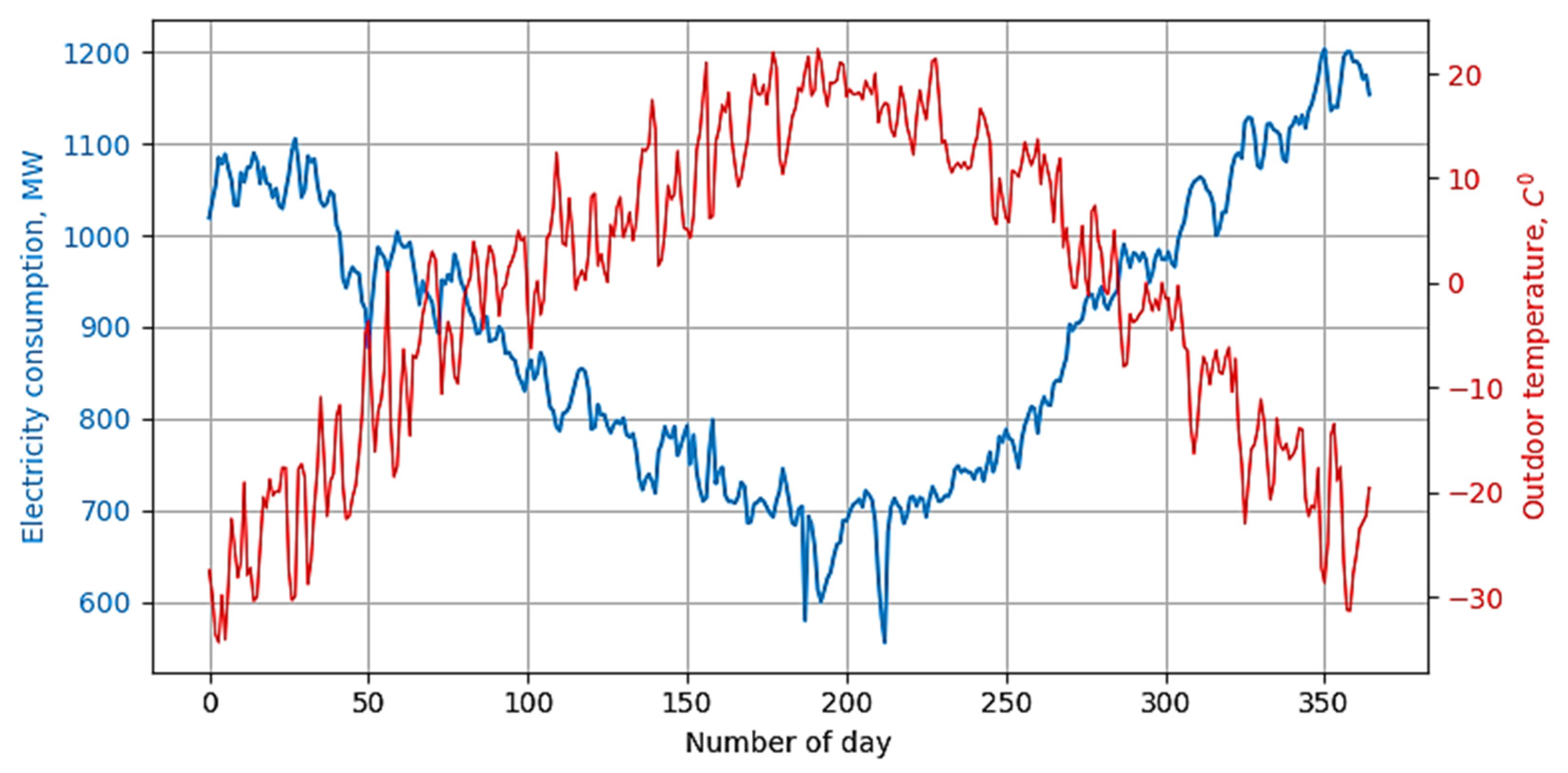
It has been established that the accurate prediction of power consumption in Mongolia requires the use of temperature forecasting; other meteorological factors have little influence on consumption.
-
It has been discovered that despite the cyclic nature of power consumption, statistical methods, such as ARIMA, are inferior to machine learning algorithms that are able to take into consideration additional factors, such as the type of day (weekends, holidays) and temperature.
The organization of this paper is as follows: Section 2 provides information about the research methods. Section 3 contains a description of the dataset and power system under consideration and the results of the research. Section 4 provides a discussion about the results. Finally, the conclusions are given in Section 5.

2. Research Methods

2.1. Autoregressive Integrated Moving Average (ARIMA) Model

The ARIMA model assumes that the forecast value is determined using a linear function of several previous values of the original time series and random errors. Modeling is implemented according to the following sequences [36].
The first stage is the calculation of the integrated component into which the data are integrated. It is achieved through subtracting each value from the previous retrospective value. The purpose of this stage is to create a time series without a trend. In other words, the time series is transformed to a stationary form from a non-stationary form to approximate modeling. There are three methods that are widely used to transform time series into stationary ones, including trend removal, seasonality, and differentiation [37]. In this paper, the differentiation method was used. The method is expressed using the following equation:
P t = P t P t 1 ,
where P t —converted value and P t —actual value.
At the next stage, autoregression is performed. It calculates the forecast value based on the weighted sum of the previous values:
P t = k = 1 p α k P t k ,
where P t is forecast value, α is the value of the weighting factor, and p is the order of the autoregression polyline.
The last step of the ARIMA is to calculate the moving average. The calculation of the moving average is performed similarly to autoregression, but errors are taken instead of actual previous values, as shown in the equation below:
u t = j = 1 q β j u t j ,
where u t is the value of the random error, β is the value of the weighting factor, and q is the order of the moving average polynomial.
As a result of the listed stages, the time series model was developed as follows.
P t = k = 1 p α k P t k + j = 1 q β j u t j .
It can be seen from the equation that the ARIMA model ( p , d , q ) is determined by the values of the polynomial degree p and q, which are calculated using the autocorrelation function (ACF) and the partial autocorrelation function (PACF) [38]. The value d reflects the number of steps required to bring the series to a stationary form. When constructing an ARIMA ( p , d , q ) time series model, it is necessary to strive to minimize the number of its parameters.

2.2. Ensemble Models

Ensemble models are machine learning algorithms that combine multiple individual models to improve the accuracy and robustness of predictions. Three popular types of ensemble models are Random Forest, AdaBoost, and XGBoost.
Random Forest is a decision tree-based ensemble model that creates multiple decision trees and aggregates their predictions to make a final prediction [39]. It is a powerful algorithm for both classification and regression tasks and is known for its ability to handle high-dimensional data with many features.
AdaBoost (Adaptive Boosting) is another ensemble model that combines weak learners to create a strong learner [40]. It works through iteratively training weak models on the same dataset and adjusting the weights of misclassified samples in each iteration to improve the overall accuracy of the model.
XGBoost (Extreme Gradient Boosting) is a gradient boosting algorithm that uses decision trees as base models [41]. It is known for its speed and scalability, making it a popular choice for large datasets. XGBoost also includes regularization techniques to prevent overfitting and improve generalization performance.
Consider a certain time series, expressed as follows:
S n = X 1 , Y 1 , X 2 , Y 2 , , X n , Y n ,
where X are the source vectors containing the functions f ( X ) ; Y are the output scalars or labels; S n are the studied samples of the time series ( X n , Y n ) with observation n .
To develop an algorithm, it is necessary to divide the data into parts for training and testing. After training on the data, the algorithm should be built with a model that calculates the dependencies between the corresponding variables. In other words, at the end of the learning process, the algorithm outputs the function h ^ X , S n of the time series model.
The basic principle of the Random Forest method is that samples of size n from the training time series S n are randomly selected and placed on the decision trees. Regression analysis and the classification of random samples are carried out on each tree, and their models are derived, which express the dependencies between random variables. The aggregation of results, which is performed via averaging the output of all decision trees, will become a Random Forest model. The main advantage of aggregation is that it is immune to outliers, since independent trees with different training samples are generated:
Y ^ = 1 q i = 1 q h ^ X , S n i ,
where S n i is i -th random sample; q is the number of the decision tree.
A model developed using the Random Forest method has the ability to take into account several factors affecting electricity consumption simultaneously. The Random Forest method contains all the advantages of machine learning methods and is preferable to the method of support vectors and neural networks since it does not require a complex theory.
To build a model with sufficient probability using this algorithm, it is necessary to specify the number of decision trees and their depth. The more decision trees, the better the probability, but the time to build a Random Forest also increases proportionally. Also, the probability of the model depends on the depth of the decision trees. Despite the fact that increasing the depth improves the quality of both training and testing, the smaller the depth of the trees, the faster this algorithm is built and works. Hence the need for an optimal choice of the number of decision trees and their depth approach.

2.3. Rank Models

Rank models allow predicting the structural properties of objects. Such tasks are quite common when calculating operating conditions and optimizing them [34]. In particular, to predict consumption in the nodes of the power system, the method of rank models is used, whose basic idea is to establish the coefficient of participation of a node in total power consumption. If we imagine the power system as a hierarchical structure with several nodes that differ in the predicted value, then we can use these models. The rank can be determined in p.u. values for tie-substations, power supply areas, power plants, and other parts of the power system. The rank is determined using the following equation:
R i = P i P ,
in which
P = i = 1 n P i ,
where P i is the forecast parameter for the ith part, P —is the total value for the object under study, R i is the rank coefficient, and n is the number of parts.
If the value of the total load or consumption is known, it can be distributed among nodes using rank coefficients. In other words, to obtain a forecast load curve for the nodes, the values of the predicted daily load profiles of the entire power system must be multiplied by the rank coefficient:
P i = P Y ^ R i ,
where P ( Y ^ ) is the value of the daily load curve of the power system, R i is the rank coefficient, and P i is the value of the daily load curve of the ith node.
If the rank remains stable at different time periods, using rank models together with other forecasting methods, it is possible to make a time series of consumption at each node. Otherwise, it is necessary to determine the rank coefficient for different time periods.
The prediction error should be measured using the average modulo error (MAE is main absolute error) and the average modulo error in percent (MAPE is main absolute percentage error). They are expressed using the following equations:
M A E = 1 N m = 1 N P m P m ,
M A P E = 1 N m = 1 N P m P m P m 100 ,
where N is number of hours in the data set, P m is the power forecast value in the m th hour, and P m is actual value in the m th hour.

3. Results

The Mongolian power system contains five regions including the central power system, which accounts for 97% of the country’s energy consumption. In 2021, the consumption of the central power system reached 9.8 million kWh, and generation—7484 million kWh. In 2021, combined heat and power (CHP) plants covered 92% of the total generation. Solar and wind power plants generated the other 8% [42,43,44]. The total installed capacity of renewable energy plants in the central power system is 268 MW, comprising 23 MW of hydropower plants, 67 MW of solar photovoltaic stations, and 155 MW of wind turbine plants. The main share of power consumption is occupied by the household sector, since industry is relatively underdeveloped. The central power system provides electricity to approximately 40 settlements. Although the mining industry has been on the rise recently, the household sector is expected to remain the leader in electricity consumption in the immediate future, according to the forecast.

3.1. The Result of the Autoregressive Integrated Moving Average Model

Any retrospective is non-stationarity by nature, since the shape of the daily load curves included in the time series is influenced by some factors. Therefore, according to the rules of analysis of the model, it is necessary to convert it to a stationary form. As an example, Figure 1 partially shows a time series of the source data. The data set is received from the system operator of the power system of Mongolia and depicts hourly load consumption.
After removing the trend and seasonality via differentiation, the time series is turned into the following pattern, as shown in Figure 2.
The initial data were divided into training and testing parts. As a training set, hourly consumption data were selected for the last 30 days before the forecast day. The analysis of autoregression and moving average was carried out on a training set, and a time series model was built. Figure 3 shows the modelled and the actual time series.
According to the developed model, the daily load curves of forecast days were predicted, which were randomly selected from each month. Since regression analysis considers the relationship between only two variables, ARIMA does not have the ability to take into account additional variables, including weather factors and other factors that affect electricity consumption.

3.2. The Result of Ensemble Models

As input data, the daily load profiles of the central power system of Mongolia were taken. These load profiles account for most of Mongolia’s electricity consumption and generation. The observation period is 1 January 2019 to 31 December 2021. Meteorological factors, including wind speed, humidity, and outdoor air temperature, were used as input data for model construction. In addition to these data, calendar features were calculated, including the type of day (weekdays and weekends) and the day of the week (Monday, Tuesday, …, Sunday) in order to reflect the difference in daily consumption.
Table 1 shows a part of the of initial data, which include the number (time), day in the week (wd), type of day (wh), outdoor temperature (temp), outdoor humidity (hum), wind speed (wind), electricity consumption (load), and electricity consumption for the i–th day ahead (load–i).
In many works regarding load forecast, the influence of individual variables listed above is investigated. In this paper, the effects of these variables are determined via correlation analysis, and the results are shown in Table 2. It can be seen that the most significant influence on electricity consumption is exerted by the outdoor air temperature, and the correlation coefficient ranges from −0.56 to −0.59, while other exogenous variables do not significantly affect consumption. In addition, it is obvious from Figure 4 that the predicted consumption significantly depends on the previous days. Thus, these factors must be considered in the development of a multifactorial model of the daily load.
To develop ensemble models, the data set is randomly divided into training and test sets in a ratio of 70 to 30. In the process of training, a list of the most influential variables is established, and a regression analysis is carried out between the predicted and actual values. Figure 5 shows the importance of the features as a measure of the relative importance of each feature in a machine learning model. The higher the feature importance score, the more important the feature is in predicting the target variable.
Figure 5 shows that the parameters of the daily load profile for forecast days depend on the previous day and prior week. As for exogenous variables, the outdoor temperature strongly influences the creation of the model. Despite the calendar features, including the type of day and the day of the week, they play their role in developing the model, but no more than the other variables considered. It is worth noting that the same behavior was observed when predicting the daily load for working days using statistical analysis in [45].
When developing algorithms, the most important task is to determine the number (n_estimators) and depth (max_depth) of decision trees included in the ensemble. The goal of the task is to set the parameters so that the quality of the model is the best, reducing the volume of the algorithm. The choice of these parameters has a significant impact on the volume of the algorithm and the probability of the model. The dependence of the model estimate on these parameters is shown in Figure 6.
From Figure 6, it is obvious that the optimal tree depth value coincides with the point at which the training score reached its maximum value, and from that moment, the test score stabilizes. In terms of the number of trees, it does not greatly affect the quality of the model, given that the model contains more than 100 trees. Thus, in order to minimize the volume of the algorithm, it is necessary to set the depth and number of trees to these values. Setting the depth and number of trees is implemented using the GridSearchCV function (sklearn library), selecting the best model parameters (Table 3).
The quality of the model was estimated using the MAE and MAPE. For the test set, MAE was 18.8 MW, and MAPE was 2.44%. Figure 7 shows the segment of the test set of the model.
The results of Random Forest, Adaptive boosting (AdaBoost), and Extreme Gradient Boosting (XGBoost) algorithms were analyzed. The results of the analysis confirm that the ensemble models have high accuracy, as shown in Table 4.
According to the constructed model, daily load profiles from each month were predicted and compared against the statistical analysis method developed in the previous work [45]. Table 4 shows the results of the ensemble models, ARIMA, and the simplest linear autoregression (AR) as a simple benchmarking method. In addition, a naïve forecast algorithm was applied (the values recorded on a previous day were used as the next-day forecast; for example, 1 p.m. is taken as the forecast for 1 p.m. for the next day).
As shown in Table 4, the machine learning method has the highest prediction accuracy with an average error of 1.25% or 10.76 MW. Therefore, this machine learning algorithm has the ability to predict power consumption with sufficient accuracy and to take into account several variables that affect load profile.

3.3. Consumption Forecasting in the Nodes of the Energy System

The central energy system of Mongolia consists of five energy supply zones, including Ulaanbaatar (energy supply zone “U”), Erdenet–Bulgan (energy supply zone “H”), Darkhan–Selenge (energy supply zone “T”), Baganuur–Choir (energy supply zone “B”) and Gov (energy supply zone “G”). Figure 8 shows the simulation network of the power system.
The daily load curves for each substation were modeled on the basis of information from the IEEE reliability testing system, where the required data were gathered via instrumentation, control, and automation equipment. Through summing up the data for the respective substations, the daily load curves of each power supply zone were calculated. Since the power system is characterized by a hierarchical structure with nodes differing in the amount of electricity consumed, the coefficients of individual node participation in the total power consumption can be determined using rank models in per-unit values. Table 5 presents the results of the rank models’ application from the point of view of the energy supply zone. The rank model parameters are visualized in Figure 9 and Figure 10.
It can be seen from Figure 10 that fairly good models have been obtained for the power supply zone according to the R2 criteria. It is worth noting that during the observations, the rank orders of rank in the studied time series did not change. Moreover, for the entire energy supply zone, fluctuations in the coefficients of participation are of small range. Hence, it can be concluded that the use of rank models allows us to precisely predict the electricity consumption in each energy supply zone.
Using machine learning methods, electricity consumption was predicted at one-hour intervals with an average error of 1.25%, and daily load curves for each energy supply zone were obtained through applying rank coefficients. As an example, Figure 11 shows the load curve for overall power consumption in the power system and load profiles per every supply zone.
It can be seen that the graphs of each energy supply zone have a different shape, since the values of the rank coefficients are constantly changing over time. In other words, the graphs show what kind of load affects the form of the total consumption curve. The final results of forecasting electricity consumption in power supply zones are shown in Table 6. Also, Figure 12 and Figure 13 depict the accuracy of the consumption model for each power supply zone. From this, it can be concluded that the proposed models can be used to calculate the operating conditions of the power system, since the average error of the models was not more than 2.0%. Also, from the point of view of power supply zones, the method can determine the loads of respective substations.

4. Discussion

The task of EPS modeling and forecasting of the processes appearing in the whole system and in its individual elements is a key objective of power system management. The solution of this task would make it possible to plan electricity generation more economically and reliably, as well as to optimize possible EPS running arrangements. However, the adopted short-term forecasting methods do not fulfill completely the needs of EPS planning and control.
The main disadvantage of the existing methods is the need to develop a load model and constantly refine the obtained model. Another disadvantage of these methods is the inaccurate determination of the relationships between input and output variables, as the dependencies between them are nonlinear. Hence, to ensure the high-quality short-term forecasting of electrical consumption in enterprises, a specific forecasting system is required. It ensures the efficient acquisition and use of the necessary data, carries out all stages of forecasting, and is controlled through a graphical user interface. The forecasting system should be adaptive, use modern methods of data analysis, and make full use of the computing power of modern computers.
This study considers the problem of modeling and forecasting the daily load profile in the nodes of a power system. A forecasting method using the coefficients of mode individual participation in the total consumption of the EPS is proposed in this work.
In the paper, the electricity consumption of the entire power system was predicted with an average error of 1.25%. The use of the machine learning method reduced the error of the ARIMA model, which was 2.58%, to 1.25%. Thus, the error reduction was 1.33 percentage points or 52%. Despite the fact that the results obtained using the ARIMA statistical method show the possibility of implementation in practice, the method is not designed to consider some important additional variables, including meteorological factors and calendar features.
For Mongolia, the proposed method of power consumption forecasting, which makes a provision for meteorological factors and is aided by machine learning algorithms and rank analysis techniques, was performed for the first time. Therefore, the results obtained are unique and cannot be found in other studies. However, the resulting accuracy is in line with state-of-the-art research in this field. The day-ahead forecasting error for large power systems is usually 1–4% [46].
The received power consumption forecast does not result in reduced electricity production since there are always standby generating capacities. But the more accurate the forecast, the more efficiently the problem of load sharing among utilities can be solved.

5. Conclusions

This paper presents techniques, such as the autoregressive integrated moving average model and a machine learning method based on the ensemble of decision trees, and demonstrates their effective use for the central power system of Mongolia for the first time in history.
This study considers the problem of modeling and forecasting the daily load profile in the nodes of the power system. The daily load curves of energy supply zones are modeled using the coefficients indicating the participation of individual nodes in total power consumption, which are established using the method of rank models. It can be concluded that the proposed models of power consumption in power supply zones can be practically applied to calculate the operating conditions of this power system, since the average error of the models was no more than 1.5%. With such accurate models, the consumption of any node of the power system can be determined using rank coefficients calculated at the appropriate level of the power system, such as tie-substations, power supply zones, and other parts of the system.
The disadvantage of the Id forecasting system is the dependence on the accuracy of meteorological forecasts, as well as the need for regular revision of power consumption coefficients for each node of the power system. The proposed approach should be generalized for other electric power systems, which is planned to be accomplished in the future.

Author Contributions

All authors have made valuable contributions to this paper. Conceptualization, T.O., P.M., M.S., I.Z. and A.R.; methodology, T.O., P.M., S.K., M.S., I.Z. and A.R.; software, P.M., T.O. and M.S.; validation, T.O., P.M., S.K. and I.Z.; formal analysis, T.O., P.M., S.K., M.S., I.Z. and A.R.; investigation, T.O., P.M., M.S. and A.R.; writing—original draft preparation, T.O., P.M., S.K., M.S., I.Z. and A.R.; writing—review and editing, T.O., S.K. and I.Z.; supervision, A.R. All authors have read and agreed to the published version of the manuscript.

Funding

The research funding from the Ministry of Science and Higher Education of the Russian Federation (Ural Federal University Program of Development within the Priority-2030 Program) is gratefully acknowledged.

Institutional Review Board Statement

Not applicable.

Informed Consent Statement

Not applicable.

Data Availability Statement

Not applicable.

Conflicts of Interest

The authors declare no conflict of interest.

References

  1. Kychkin, A.V.; Chasparis, G.C. Feature and model selection for day-ahead electricity-load forecasting in residential buildings. Energy Build. 2021, 249, 111200. [Google Scholar] [CrossRef]
  2. Alfares, H.K.; Nazeeruddin, M. Electric load forecasting: Literature survey and classification of methods. Int. J. Syst. Sci. 2002, 33, 23–34. [Google Scholar] [CrossRef]
  3. Ghalehkhondabi, I.; Ardjmand, E.; Weckman, G.R.; Young, W.A. An overview of energy demand forecasting methods published in 2005–2015. Energy Syst. 2017, 2, 411–447. [Google Scholar] [CrossRef]
  4. Abdurahmanov, A.; Volodin, M.; Zybin, E.; Ryabchenko, V. Forecasting methods in electricity distribution networks (review). Russ. Internet J. Electr. Eng. 2016, 3, 3–23. [Google Scholar] [CrossRef]
  5. Patel, H.; Shah, M. Energy Consumption and Price Forecasting Through Data-Driven Analysis Methods: A Review. SN Comput. Sci. 2021, 2, 315. [Google Scholar] [CrossRef]
  6. Makoklyuev, B.I. Analysis and Planning of Electricity Consumption; Energoatomizdat: Moscow, Russia, 2008. [Google Scholar]
  7. Matrenin, P.; Antonenkov, D.; Arestova, A. Energy Efficiency Improvement of Industrial Enterprise Based on Machine Learning Electricity Tariff Forecasting. In Proceedings of the 2021 15th International Scientific-Technical Conference on Actual Problems of Electronic Instrument Engineering, APEIE 2021, Novosibirsk, Russia, 19–21 November 2021. [Google Scholar] [CrossRef]
  8. Matrenin, P.V.; Manusov, V.Z.; Khalyasmaa, A.I.; Antonenkov, D.V.; Eroshenko, S.A.; Butusov, D.N. Improving Accuracy and Generalization Performance of Small-Size Recurrent Neural Networks Applied to Short-Term Load Forecasting. Mathematics 2020, 8, 2169. [Google Scholar] [CrossRef]
  9. Kamalov, F.; Smail, L.; Gurrib, I. Stock price forecast with deep learning. In Proceedings of the 2020 International Conference on Decision Aid Sciences and Application (DASA), Sakheer, Bahrain, 8–9 November 2020; pp. 1098–1102. [Google Scholar]
  10. Chen, Y.; Tang, Y.; Zhang, S.; Liu, G.; Liu, T. Weather Sensitive Residential Load Forecasting Using Neural Networks. In Proceedings of the 2023 IEEE 6th International Electrical and Energy Conference (CIEEC), Hefei, China, 12–14 May 2023. [Google Scholar] [CrossRef]
  11. Xu, F.; Xu, W.; Qiu, Y.; Wu, M.; Wang, R.; Li, Y.; Fan, P.; Yang, J. A Short-term Load Forecasting Model Based on Neural Network Considering Weather Features. In Proceedings of the 2021 IEEE 4th International Conference on Automation, Electronics and Electrical Engineering (AUTEEE), Shenyang, China, 19–21 November 2021. [Google Scholar] [CrossRef]
  12. Chodakowska, E.; Nazarko, J.; Nazarko, Ł. ARIMA Models in Electrical Load Forecasting and Their Robustness to Noise. Energies 2021, 14, 7952. [Google Scholar] [CrossRef]
  13. López, J.C.; Rider, M.J.; Wu, Q. Parsimonious Short-Term Load Forecasting for Optimal Operation Planning of Electrical Distribution Systems. IEEE Trans. Power Syst. 2019, 34, 1427–1437. [Google Scholar] [CrossRef]
  14. Sun, X.; Luh, P.B.; Cheung, K.W.; Guan, W.; Michel, L.D.; Venkata, S.S.; Miller, M.T. An efficient approach to short-term load forecasting at the distribution level. IEEE Trans. Power Syst. 2015, 31, 2526–2537. [Google Scholar] [CrossRef]
  15. Fernandes, K.C.; Sardinha, R.; Rebelo, S.; Singh, R. Electric load analysis and forecasting using artificial neural networks. In Proceedings of the 2019 3rd International Conference on Trends in Electronics and Informatics (ICOEI), Tirunelveli, India, 23–25 April 2019; pp. 1274–1278. [Google Scholar] [CrossRef]
  16. Alobaidi, M.H.; Chebana, F.; Meguid, M.A. Robust ensemble learning framework for day—Ahead forecasting of household based energy consumption. Appl. Energy 2018, 212, 997–1012. [Google Scholar] [CrossRef]
  17. Shi, J.; Wang, Z. A Hybrid Forecast Model for Household Electric Power by Fusing Landmark-Based Spectral Clustering and Deep Learning. Sustainability 2022, 14, 9255. [Google Scholar] [CrossRef]
  18. Huyghues-Beaufond, N.; Tindemans, S.; Falugi, P.; Sun, M.; Strbac, G. Robust and automatic data cleansing method for short-term load forecasting of distribution feeders. Appl. Energy 2020, 261, 114405. [Google Scholar] [CrossRef]
  19. Hayes, B.P.; Gruber, J.K.; Prodanovic, M. Multi-nodal short-term energy forecasting using smart meter data. IET Gener. Transm. Distrib. 2018, 12, 2988–2994. [Google Scholar] [CrossRef]
  20. Tan, M.; Hu, C.; Chen, J.; Wang, L.; Li, Z. Multi-node load forecasting based on multi-task learning with modal feature extraction. Eng. Appl. Artif. Intell. 2022, 112, 104856. [Google Scholar] [CrossRef]
  21. Tan, M.; Liu, Y.; Meng, B.; Su, Y. Multinodal forecasting of industrial power load using participation factor and ensemble learning. In Proceedings of the 2020 IEEE 4th Conference on Energy Internet and Energy System Integration (EI2), Wuhan, China, 30 October–1 November 2020; pp. 745–750. [Google Scholar] [CrossRef]
  22. Abreu, T.; Amorim, A.J.; Santos-Junior, C.R.; Lotufo, A.D.; Minussi, C.R. Multinodal load forecasting for distribution systems using a fuzzy-artmap neural network. Appl. Soft Comput. 2018, 71, 307–316. [Google Scholar] [CrossRef]
  23. Rai, S.; De, M. Effect of Load Contribution Factor on Multinodal Load Forecasting. In Proceedings of the IEEE EUROCON 2021—19th International Conference on Smart Technologies, Lviv, Ukraine, 6–8 July 2021; pp. 455–459. [Google Scholar] [CrossRef]
  24. Amorim, A.J.; Abreu, T.A.; Tonelli-Neto, M.S.; Minussi, C.R. A new formulation of multinodal short-term load forecasting based on adaptive resonance theory with reverse training. Electr. Power Syst. Res. 2020, 179, 106096. [Google Scholar] [CrossRef]
  25. Ferreira, A.B.A.; Minussi, C.R.; Lotufo, A.D.P.; Lopes, M.L.M.; Chavarette, F.R.; Abreu, T.A. Multinodal load forecast using euclidean ARTMAP Neural network. In Proceedings of the 2019 IEEE PES Innovative Smart Grid Technologies Conference-Latin America (ISGT Latin America), Gramado, Brazil, 15–18 September 2019; pp. 1–6. [Google Scholar] [CrossRef]
  26. Stephen, B.; Telford, R.; Galloway, S. Non-Gaussian residual based short term load forecast adjustment for distribution feeders. IEEE Access 2020, 8, 10731–10741. [Google Scholar] [CrossRef]
  27. Stephen, B.; Tang, X.; Harvey, P.R.; Galloway, S.; Jennett, K.I. Incorporating practice theory in sub-profile models for short term aggregated residential load forecasting. IEEE Trans. Smart Grid 2015, 8, 1591–1598. [Google Scholar] [CrossRef]
  28. Wang, J.; Zhu, W.; Zhang, W.; Sun, D. A trend fixed on firstly and seasonal adjustment model combined with the ε-SVR for short-term forecasting of electricity demand. Energy Policy 2009, 37, 4901–4909. [Google Scholar] [CrossRef]
  29. Çevik, H.H.; Çunkaş, M. Short-term load forecasting using fuzzy logic and ANFIS. Neural Comput. Appl. 2015, 26, 1355–1367. [Google Scholar] [CrossRef]
  30. Lahouar, A.; Slama, J.B.H. Day-ahead load forecast using random forest and expert input selection. Energy Convers. Manag. 2015, 103, 1040–1051. [Google Scholar] [CrossRef]
  31. Moon, J.; Kim, Y.; Son, M.; Hwang, E. Hybrid short-term load forecasting scheme using random forest and multilayer perceptron. Energies 2018, 11, 3283. [Google Scholar] [CrossRef]
  32. Lahouar, A.; Slama, J.B.H. Hour-ahead wind power forecast based on random forest. Renew. Energy 2017, 109, 529–541. [Google Scholar] [CrossRef]
  33. Barrows, C.; Bloom, A.; Ehlen, A.; Ikaheimo, J.; Jorgenson, J.; Krishnamurthy, D.; Lau, J.; McBennett, B.; O’Connell, M.; Preston, E. The IEEE reliability test system: A proposed 2019 update. IEEE Trans. Power Syst. 2019, 35, 119–127. [Google Scholar] [CrossRef]
  34. Saranchimeg, S.; Nair, N.K.C. A novel framework for integration analysis of large-scale photovoltaic plants into weak grids. Appl. Energy 2021, 282, 116141. [Google Scholar] [CrossRef]
  35. Rusina, A.G.; Sidorkin, Y.M.; Kalinin, A.E. Application of rank models for structural forecasting. In Proceedings of the 2016 11th International Forum on Strategic Technology (IFOST 2016), Novosibirsk, Russia, 1–3 June 2016; pp. 271–275. [Google Scholar] [CrossRef]
  36. Velasco, L.C.P.; Polestico, D.L.L.; Macasieb, G.P.O.; Reyes, M.B.V.; Vasquez, F.B., Jr. Load forecasting using autoregressive integrated moving average and artificial neural network. Int. J. Adv. Comput. Sci. Appl. 2018, 9, 23–29. [Google Scholar] [CrossRef]
  37. Kamalov, F. A note on time series differencing. Gulf J. Math. 2021, 10, 50–56. [Google Scholar] [CrossRef]
  38. Kamalov, F. A note on the autocovariance of p-series linear process. Gulf J. Math. 2020, 9, 40–45. [Google Scholar] [CrossRef]
  39. Breiman, L. Random Forests. Mach. Learn. 2001, 4, 5–32. [Google Scholar] [CrossRef]
  40. Chen, T.; Guestrin, C. XGBoost: A Scalable Tree Boosting System. Available online: https://arxiv.org/abs/1603.02754 (accessed on 22 May 2023).
  41. Drucker, H. Improving Regressors Using Boosting Techniques. Available online: http://citeseerx.ist.psu.edu/viewdoc/download?doi=10.1.1.31.314&rep=rep1&type=pdf (accessed on 22 May 2023).
  42. Matrenin, P.V.; Osgonbaatar, T.; Sergeev, N.N. Overview of Renewable Energy Sources in Mongolia. In Proceedings of the 2022 IEEE International Multi-Conference on Engineering, Computer and Information Sciences (SIBIRCON), Yekaterinburg, Russia, 11–13 November 2022. [Google Scholar] [CrossRef]
  43. Bumtsend, U.; Safaraliev, M.; Ghulomzoda, A.; Ghoziev, B.; Ahyoev, J.; Ghulomabdolov, G. The Unbalanced Modes Analyze of Traction Loads Network. In Proceedings of the 2020 Ural Symposium on Biomedical Engineering, Radioelectronics and Information Technology (USBEREIT), Yekaterinburg, Russia, 14–15 May 2020; pp. 0456–0459. [Google Scholar] [CrossRef]
  44. Manusov, V.Z.; Bumtsend, U.; Demin, Y.V. Analysis of the power quality impact in power supply system of Urban railway passenger transportation—The city of Ulaanbaatar. IOP Conf. Ser. Earth Environ. Sci. 2018, 177, 012024. [Google Scholar]
  45. Vivas, E.; Allende-Cid, H.; Salas, R. A Systematic Review of Statistical and Machine Learning Methods for Electrical Power Forecasting with Reported MAPE Score. Entropy 2020, 22, 1412. [Google Scholar] [CrossRef]
  46. Rusina, A.G.; Tuvshin, O.; Matrenin, P.V. Forecasting the daily energy load schedule of working days using meteofactors for the central power system of Mongolia. Power Eng. Res. Equip. Technol. 2022, 24, 98–107. [Google Scholar] [CrossRef]
Figure 1. Example of a time series of source data.
Inventions 08 00114 g001
Figure 2. Transformed time series.
Inventions 08 00114 g002
Figure 3. Time series modeling.
Inventions 08 00114 g003
Figure 4. Graph of average daily consumption and average daily temperature for 2021.
Inventions 08 00114 g004
Figure 5. The role of initial variables in the learning process.
Inventions 08 00114 g005
Figure 6. Dependence of the model probability on the depth and number of trees.
Inventions 08 00114 g006aInventions 08 00114 g006b
Figure 7. The segment of the model testing process.
Inventions 08 00114 g007
Figure 8. Simulation network representing the central power system of Mongolia.
Inventions 08 00114 g008
Figure 9. Rank model for the power supply zone.
Inventions 08 00114 g009
Figure 10. Dependence between rank coefficient and rank number.
Inventions 08 00114 g010
Figure 11. Daily load curves of the power system and power supply zones.
Inventions 08 00114 g011
Figure 12. Rank model for the power supply zone.
Inventions 08 00114 g012
Figure 13. Accuracy of consumption models of power supply zones.
Inventions 08 00114 g013
Table 1. Fragment of initial data.
YearMonthDayHourWdWhTempHumWindLoad-7Load-6Load-1
201918021−33673947894917
201918131−31685888838850
201918231−29684825825819
201918331−33674795811813
201918431−33675773808804
Table 2. Correlation values between initial and forecasting data.
 WdWhWindHumTempLoad-7Load-6Load-5Load-4Load-3Load-2Load-1
load0.0040.050.15−0.03−0.590.960.960.960.970.970.970.98
Table 3. Hyperparameters of models.
 Random ForestAdaBoostXGBoost
Depth of trees121212
Number of trees100100100
MAPE [%]2.442.382.35
Table 4. Forecasting accuracy.
MonthNaiveARARIMARandom ForestAdaBoostXG Boost
 MAE
[MW]
MAPE
[%]
MAE [MW]MAPE [%]MAE [MW]MAPE [%]MAE [MW]MAPE [%]MAE [MW]MAPE [%]MAE [MW]MAPE [%]
January20.901.9726.112.4519.901.9010.240.9210.821.045.840.55
February26.542.7023.122.2133.703.0516.671.6313.731.3311.381.11
March20.532.2331.293.2625.862.6425.042.6611.701.239.380.97
April20.222.4526.423.1720.062.229.801.3210.451.268.751.02
May22.762.9829.513.9828.263.8816.622.2611.081.479.431.26
June27.043.6711.681.6928.254.067.691.1712.651.8012.031.70
July30.195.5411.731.7819.913.0511.201.668.641.316.891.06
August22.693.2133.184.5215.062.088.871.2119.362.649.251.24
September24.092.9823.783.0317.212.148.911.0816.642.1715.542.09
October19.642.0743.284.6121.812.4611.931.2718.391.9317.481.79
November22.512.1421.762.1818.611.9314.311.3715.521.5814.831.48
December20.291.7830.532.8317.391.669.200.8710.690.968.330.76
Result23.142.8126.032.9622.172.5912.541.4513.261.5610.761.25
Table 5. Results of rank models.
Name
of the Energy Supply Zone
Name
of the Calculation
Rank NumberPercentage of the Total Power Load
Participation Rate, %
Ulaanbaatar‘U’I54.34
Erdenet-Bulgan‘H’II25.73
Darkhan-Selenge‘T’III8.75
Frog‘B’IV8.63
Gobi‘G’V2.55
Table 6. Final results of consumption forecasting in energy supply zones.
Rank NumberZone UZone HZone BZone TZone G
MAE [MW]MAPE
[%]
MAE [MW]MAPE
[%]
MAE [MW]MAPE
[%]
MAE [MW]MAPE
[%]
MAE [MW]MAPE
[%]
January2.810.370.830.370.410.480.380.490.291.38
February7.701.242.521.271.041.210.861.180.311.46
March3.690.581.160.560.490.560.540.700.231.29
April8.051.663.361.651.661.831.151.680.241.86
May1.380.320.600.340.300.400.250.410.151.43
June2.550.661.180.700.570.780.480.690.161.46
July5.051.432.411.430.901.340.941.370.181.48
August6.731.582.461.591.141.581.111.600.302.12
September1.370.320.620.370.290.410.240.350.221.78
October3.560.801.440.800.580.840.550.860.221.41
November6.681.392.651.411.061.370.951.400.331.79
December1.770.310.720.360.350.460.370.490.231.10
Result4.20.881.660.900.730.930.650.930.231.54
Disclaimer/Publisher’s Note: The statements, opinions and data contained in all publications are solely those of the individual author(s) and contributor(s) and not of MDPI and/or the editor(s). MDPI and/or the editor(s) disclaim responsibility for any injury to people or property resulting from any ideas, methods, instructions or products referred to in the content.

