Effect of Support Stiffness Nonlinearity on the Low-Frequency Vibro-Acoustic Characteristics for a Mechanical Equipment—Floating Raft—Underwater Cylindrical Shell Coupled System

Abstract

The low-frequency vibro-acoustic characteristics of a mechanical equipment—floating raft—cylindrical shell—underwater acoustic field coupled system with nonlinear supports are studied in this paper. Firstly, the state space equations were established by a modal superposition theory for the coupled system, and a modal parameter identification method was deduced and verified for the cylindrical shell—underwater acoustic field coupled subsystem. On this basis, the formulas were derived for transmitted power flow in the coupled system, and the nonlinear stiffness constitutive relation of the vibration isolation supports was expressed by softening and hardening characteristics. Finally, dynamic simulations were carried out by the Runge—Kutta method to analyze the effect of nonlinear stiffness characteristic parameters on the low-frequency vibration modes and vibro-acoustic transfer characteristics in the coupled system. The research shows that a superharmonic phenomenon is common in the steady vibration mode of the coupled system with a nonlinear softening (or hardening) stiffness characteristic under harmonic excitation. The stronger the softening (or hardening) stiffness characteristic is, the more complex the vibration form is, and the smaller (or larger) the low-frequency vibro-acoustic transfer level in resonance regions is.

1. Introduction

Nonlinear vibration mode is an important factor to be considered in the study of low-frequency vibration isolation for underwater cylindrical shell systems. Due to relatively high vibration energy at low frequencies, the elastic support, which presents linear stiffness in an original micro-amplitude vibration mode, will show nonlinear characteristics. Strictly speaking, stiffness characteristics of various elastic vibration isolation elements are nonlinear. In a micro-amplitude vibration mode, a vibration isolator has a certain linear stiffness working interval. Stiffness characteristics are nonlinear if amplitude is sufficiently large.

In recent years, many scholars have studied the vibration characteristics of nonlinear vibration isolation systems. Smirnov et al. [1] studied and compared the efficiency of linear and nonlinear vibration isolation systems. Santhosh [2] studied the dynamic performance of an asymmetric nonlinear vibration isolation mechanism under harmonic excitation. Dutta et al. [3] analyzed a nonlinear vibration isolator with magnetorheological fluid dampers and cubic nonlinear springs to determine the effectiveness of isolation during force or displacement excitation. Suman et al. [4] proposed a nonlinear vibration control device based on a negative stiffness mechanism, which can improve the isolation ability of the vibration suspension system in the low-frequency range. Araki et al. [5] proposed a vertical quasi-zero stiffness (QZS) vibration isolator with adjustable restoring force. Zhao et al. [6,7] successively designed QZS vibration isolators with two and three pairs of inclined springs. Ye et al. [8] proposed a QZS system based on a cam—roller mechanism. Chang et al. [9] proposed a QZS dynamic shock absorber. Bouna et al. [10] studied the vibration control of multi-span girder bridges under the excitation of pier foundation vibration by using nonlinear QZS isolators. Drezet et al. [11] proposed a nonlinear vibration energy harvester based on the concept of high static and low dynamic stiffness (HSLDS). Lu et al. [12,13,14] studied an orthogonal six-degree-of-freedom vibration isolation system with HSLDS and an electromagnetic Stewart platform to suppress the low-frequency vibration of high-precision instruments, provided modal coefficients by improved Fourier series and the Rayleigh—Ritz method, and studied the nonlinear energy transfer of flexible plates with arbitrary boundaries coupled to HSLDS isolators. Sun et al. [15] proposed a method for designing HSLDS mounts based on target force curves, which are obtained by placing negative stiffness structures in parallel with positive stiffness linear springs. Yao et al. [16] proposed an HSLDS isolator with a cam—roller—spring mechanism, in which the cam profile can be specially designed to suit different operating requirements. Chong et al. [17] designed a nonlinear X-combined structure with HSLDS in a large displacement range, which avoided negative stiffness and instability factors and improved its vibration isolation characteristics.

Chaos is a unique dynamical behavior of nonlinear systems. Leutcho et al. [18] systematically studied a new type of chaotic system with single parametric nonlinearity. Yan et al. [19] proposed a novel bi-state nonlinear vibration isolator, whose motion can be either periodic or chaotic. Rahman et al. [20] proposed a new fractional-order chaotic system containing multiple nonlinear terms, which can excite hidden chaotic attractors or self-excited chaotic attractors depending on the chosen system parameters or the value of its fractional-order derivative. Li et al. [21] proposed an SRN feature extraction method combining maximum relevance minimum redundancy, which can effectively classify different chaotic signals. Karimov et al. [22] proposed a novel implementation of the chaotic Duffing oscillator as a simple mechanical system with a translational movement. Dreau et al. [23] introduced a stochastic modeling method for nonlinear systems with response surface discontinuity, which improved the efficiency of multi-variate polynomial chaos expansion.

The power flow characteristic is an important index to study nonlinear vibration isolation. Cassidy et al. [24] proposed a general nonlinear control synthesis method for power flow constrained energy harvesters, which is analytically guaranteed to be superior to the optimal static admittance in the steady state random response. Silva et al. [25] proposed a technique for evaluating and optimizing vibrational power flow involving beam-and-plate coupling. Varghese et al. [26] applied the combined transient power flow balancing and acceleration matching techniques to detect and quantify the crack damage of beam structures at different positions. Yang et al. [27,28] successively studied the power flow and force transmissibility characteristics of a two-degree-of-freedom nonlinear vibration isolation system and a coupled nonlinear oscillator. Ren et al. [29] compared the power transmission between rigid, single-stage isolation and double-stage isolation gearbox installation configurations with the vibration power flow of the system as the evaluation index. Zhang et al. [30] proposed a power flow analysis method for quantitatively evaluating the dynamic performance of a nonlinear energy sink in the frequency domain. Xu et al. [31] analyzed the bending vibration and power flow of axially loaded beams with arbitrary boundaries and nonuniform elastic foundations via energy principle in conjunction with the Rayleigh—Ritz procedure. Mahapatra et al. [32] studied the influence of general coupling conditions on the vibration and power flow characteristics of a two-plate composite plate structure.

There has been a lot of literature on the dynamics of nonlinear vibration isolation systems at home and abroad and, especially, the application of quasi-zero stiffness or high static and low dynamic stiffness nonlinear vibration isolators for low-frequency vibration control has become a research hotspot in the last decade. However, compared with the wide application of nonlinear vibration isolators, the mechanism of vibro-acoustic transfer in nonlinear vibration isolation systems, especially the influence of nonlinear factors in low-frequency vibration modes, has not been fully studied. In this paper, the low-frequency vibro-acoustic characteristics of a mechanical equipment—floating raft—underwater cylindrical shell coupled system with nonlinear stiffness supports are studied. It can not only provide theoretical guidance for low-frequency vibration analysis, diagnosis, and design of dynamics of underwater nonlinear coupled systems but also provide reference for the design of nonlinear vibration isolators.

The rest of this paper is organized as follows. In Section 2, based on the parametric modeling of an admittance method of a mechanical equipment—floating raft—cylindrical shell—underwater acoustic field coupled system, the state space equations of the subsystems are established by using modal identification and modal superposition theories; and then the nonlinear stiffness constitutive relation of the vibration isolation supports is expressed by softening and hardening characteristics, and the calculation method of transmitted power flow is derived. In Section 3, the influence of nonlinear stiffness characteristic parameters on the vibro-acoustic characteristics of the coupled system is studied by using MATLAB numerical simulation. Finally, some conclusions are presented in Section 4.

2. Materials and Methods

2.1. Model of a Mechanical Equipment—Floating Raft—Cylindrical Shell—Underwater Acoustic Field Coupled System

Figure 1 describes the model of a mechanical equipment—floating raft—cylindrical shell—underwater acoustic field coupled system.

As shown in Figure 1a,b, vibration source mechanical equipment A₁ and A₂ (simulating multiple units) are installed on a floating raft R. Each unit is connected to the raft frame through four elastic supports, and the raft frame is connected to a cylindrical shell through four elastic supports. A rectangular coordinate system Oxyz is established, where the Oz axis is the center line of the cylinder and Oy is the vertical direction. To simplify analysis, only the vertical translational vibration and the rotational vibration around the Oz and Ox axes of the system are considered. Therefore, vertical excitation forces F₁, F₂ and excitation torques T₁, T₂ around the Oz axis are applied at the center of mass of each unit. The units A₁, A₂ and the floating raft R are all rigid bodies symmetrical about the yOz plane. In Figure 1a,b, b₁, b₂, h_1z, h_2z, h_1x, h_2x, H_z, H_x, and L_R are the installation size parameters of the system, and σ₁, σ₂, σ₃, and σ₄ are the connection points of the lower vibration isolation supports with the cylindrical shell.

Figure 1c abstracts the complex coupled system with nonlinear connecting elements. A (the vibration source subsystem) is subjected to l excitations F_en (n = 1, 2, …, l) and has displacement responses w_en at the excitations. A is connected to R (the raft frame) by q elastic connecting elements. At the connection points of the elastic elements with A and R, there are excitation forces F_Ai and F_ti (i = 1, 2, …, q), as well as displacement responses w_Ai and w_ti. The elastic elements have constitutive relation f_i(δ_i, ${\dot{\delta }}_i$), where δ_i = w_Ai − w_ti. Similarly, R is connected to Y (the cylindrical shell–underwater acoustic field coupled subsystem) by r elastic connecting elements. At the connection points of the elastic elements with R and Y, there are excitation forces F_bj and F_yj (j = 1, 2, …, r), as well as displacement responses w_bj and w_yj. The elastic elements have constitutive relation g_j(κ_j, ${\dot{\kappa }}_j$), where κ_j = w_bj − w_yj. For specific practical problems, the number of elastic coupled elements in series in Figure 1c can be increased or decreased according to different modeling needs.

2.2. State Space Model of the Coupled System

For the unit A₁ in Figure 1, its vertical vibration displacement is represented by y₁; its angular displacement around the Ox axis is represented by θ_1x; and its angular displacement around the Oy axis is represented by θ_1y. Define a state variable u_A1 = [u₁, u₂, u₃, u₄, u₅, u₆]^T = [y₁, θ_1x, θ_1z, ${\dot{y}}_1$, ${\dot{\theta }}_{1x}$, ${\dot{\theta }}_{1z}$]^T, then the state space of the unit A₁ equation is

$${\dot{\mathit{u}}}_{\mathrm{A}1}=\left[\begin{array}{c}{\dot{u}}_1\\ {\dot{u}}_2\\ {\dot{u}}_3\\ {\dot{u}}_4\\ {\dot{u}}_5\\ {\dot{u}}_6\end{array}\right]=\left[\begin{array}{cccccc}0& 0& 0& 1& 0& 0\\ 0& 0& 0& 0& 1& 0\\ 0& 0& 0& 0& 0& 1\\ 0& 0& 0& 0& 0& 0\\ 0& 0& 0& 0& 0& 0\\ 0& 0& 0& 0& 0& 0\end{array}\right]\left[\begin{array}{c}{u}_1\\ u_2\\ u_3\\ u_4\\ u_5\\ u_6\end{array}\right]+\left[\begin{array}{c}0\\ 0\\ 0\\ -{\mathit{I}}_{1\times 4}·{\mathit{F}}_1/m_1\\ {\mathit{Z}}_1·{\mathit{F}}_1/J_{1x}\\ -{\mathit{X}}_1·{\mathit{F}}_1/J_{1z}\end{array}\right]+\left[\begin{array}{c}0\\ 0\\ 0\\ F_1/m_1\\ 0\\ T_1/J_{1z}\end{array}\right]={\Lambda }_0·u_{\mathrm{A}1}+f_{\mathrm{A}1}\left(F_1\right)+f_{\mathrm{in}1}\left(t\right)$$

(1)

where F₁ = [F_A1, F_A2, F_A3, F_A4]^T is an excitation force column vector of the unit A₁ to its four supports; m₁, J_1x, and J_1z are the mass of the unit A₁ and the moment of inertia that bypasses its centroid and is parallel to the axis of Ox and Oz, respectively; X₁ = [0.5h_1x, 0.5h_1x, −0.5h_1x, −0.5h_1x]; Z₁ = [−0.5h_1z, 0.5h_1z, −0.5h_1z, 0.5h_1z]; I_1×4 denotes a 4-dimensional row vector with all elements 1; f_A1(F₁) denotes a vector function with respect to F₁; f_in1 is a known external input vector function; Λ₀ is a constant matrix.

Similarly, for the unit A₂, its vertical vibration displacement is represented by y₂; its angular displacement around the Ox axis is represented by θ_2x; and its angular displacement around the Oy axis is represented by θ_2y. Define a state variable u_A2 = [u₇, u₈, u₉, u₁₀, u₁₁, u₁₂]^T = [y₂, θ_2x, θ_2z, ${\dot{y}}_2$, ${\dot{\theta }}_{2x}$, ${\dot{\theta }}_{2z}$]^T, then the state space equation of the unit A₂ is

$${\dot{u}}_{\mathrm{A}2}={\Lambda }_0·u_{\mathrm{A}2}+f_{\mathrm{A}2}\left(F_2\right)+f_{\mathrm{in}2}\left(t\right)$$

(2)

where F₂ = [F_A5, F_A6, F_A7, F_A8]^T is an excitation force column vector of the unit A₂ to its four supports; f_A2(F₂) = [0, 0, 0, −I_1×4⋅F₂/m₂, Z₂⋅F₂/J_2x, −X₂⋅F₂/J_2z]^T denotes a vector function with respect to F₂; f_in2 = [0, 0, 0, F₂/m₂, 0, T₂/J_2z]^T is a known external input vector function; m₂, J_2x, and J_2z are the mass of the unit A₂ and the moment of inertia that bypasses its centroid and is parallel to the axis of Ox and Oz, respectively; X₂ = [0.5h_2x, 0.5h_2x, −0.5h_2x, −0.5h_2x]; Z₂ = [−0.5h_2z, 0.5h_2z, −0.5h_2z, 0.5h_2z].

Combining the units A₁ and A₂ into the vibration source equipment subsystem, Equations (1) and (2) are merged into the following state space equation:

$${\dot{u}}_{\mathrm{A}}=\left[\begin{array}{c}{\dot{u}}_{\mathrm{A}1}\\ {\dot{u}}_{\mathrm{A}2}\end{array}\right]=\left[\begin{array}{cc}{\Lambda }_0& O_{6\times 6}\\ O_{6\times 6}& {\Lambda }_0\end{array}\right]\left[\begin{array}{c}{u}_{\mathrm{A}1}\\ u_{\mathrm{A}2}\end{array}\right]+\left[\begin{array}{c}{f}_{\mathrm{A}1}\left(F_1\right)\\ f_{\mathrm{A}2}\left(F_2\right)\end{array}\right]+\left[\begin{array}{c}{f}_{\mathrm{in}1}\left(t\right)\\ f_{\mathrm{in}2}\left(t\right)\end{array}\right]=\Lambda ·u_{\mathrm{A}}+f_{\mathrm{A}}\left(F_1,F_2\right)+f_{\mathrm{in}}\left(t\right)$$

(3)

For the raft frame R, its vertical vibration displacement is represented by y_R; its angular displacement around the Ox axis is represented by θ_Rx; and its angular displacement around the Oy axis is represented by θ_Ry. Define a state variable u_R = [u_R1, u_R2, u_R3, u_R4, u_R5, u_R6]^T = [y_R, θ_Rx, θ_Rz, ${\dot{y}}_{\mathrm{R}}$, ${\dot{\theta }}_{\mathrm{R}x}$, ${\dot{\theta }}_{\mathrm{R}z}$]^T, then the state space equation of the raft frame R is

$${\dot{u}}_{\mathrm{R}}=\left[\begin{array}{c}{\dot{u}}_{\mathrm{R}1}\\ {\dot{u}}_{\mathrm{R}2}\\ {\dot{u}}_{\mathrm{R}3}\\ {\dot{u}}_{\mathrm{R}4}\\ {\dot{u}}_{\mathrm{R}5}\\ {\dot{u}}_{\mathrm{R}6}\end{array}\right]=\left[\begin{array}{cccccc}0& 0& 0& 1& 0& 0\\ 0& 0& 0& 0& 1& 0\\ 0& 0& 0& 0& 0& 1\\ 0& 0& 0& 0& 0& 0\\ 0& 0& 0& 0& 0& 0\\ 0& 0& 0& 0& 0& 0\end{array}\right]\left[\begin{array}{c}{u}_{\mathrm{R}1}\\ u_{\mathrm{R}2}\\ u_{\mathrm{R}3}\\ u_{\mathrm{R}4}\\ u_{\mathrm{R}5}\\ u_{\mathrm{R}6}\end{array}\right]+\left[\begin{array}{c}0\\ 0\\ 0\\ I_{1\times 8}·\left(F_{\mathrm{t}}-F_{\mathrm{b}}\right)/m_{\mathrm{R}}\\ \left(Z_{\mathrm{R}2}·F_{\mathrm{b}}-Z_{\mathrm{R}1}·F_{\mathrm{t}}\right)/J_{\mathrm{R}x}\\ \left(X_{\mathrm{R}1}·F_{\mathrm{t}}-X_{\mathrm{R}2}·F_{\mathrm{b}}\right)/J_{\mathrm{R}z}\end{array}\right]={\Lambda }_0·u_{\mathrm{R}}+f_{\mathrm{R}}\left(F_{\mathrm{t}},F_{\mathrm{b}}\right)$$

(4)

where F_t = [F_t1, F_t2, F_t3, F_t4, F_t5, F_t6, F_t7, F_t8]^T and F_b = [F_b1, F_b2, F_b3, F_b4]^T are excitation force column vectors of the upper supports to the raft frame and the raft frame to the lower supports, respectively; m_R, J_Rx, and J_Rz are the mass of the raft frame and the moment of inertia that bypasses its centroid and is parallel to the axis of Ox and Oz, respectively; X_R1 = [0.5h_1x, 0.5h_1x, −0.5h_1x, −0.5h_1x, 0.5h_2x, 0.5h_2x, −0.5h_2x, −0.5h_2x]; X_R2 = [0.5H_x, 0.5H_x, −0.5H_x, −0.5H_x]; Z_R1 = [−b₁ − 0.5h_1z, −b₁ + 0.5h_1z, −b₁ − 0.5h_1z, −b₁ + 0.5h_1z, b₂ − 0.5h_2z, b₂ + 0.5h_2z, b₂ − 0.5h_2z, b₂ + 0.5h_2z]; Z_R2 = [−0.5H_z, 0.5H_z, −0.5H_z, 0.5H_z]; f_R(F_t, F_b) denotes a vector function about F_t, F_b.

For the connection supports between the vibration source equipment and the raft frame, ignoring the effect of their mass, the power/response transfer relation is

$$F_{\mathrm{t}i}=F_{\mathrm{A}i}=f_i({\delta }_i, {\dot{\delta }}_i), \left(i=1, 2, \dots , 8\right)$$

(5)

where δ_i = w_Ai − w_ti, and there are linear relationships between w_Ai, w_ti and the state variables u_A and u_R:

$$\left\{\begin{array}{c}\begin{array}{cc}{w}_{\mathrm{A}1}=u_1{I}_{4\times 1}-u_2{Z}_1^{\mathrm{T}}+u_3{X}_1^{\mathrm{T}},& {\dot{w}}_{\mathrm{A}1}=u_4{I}_{4\times 1}-u_5{Z}_1^{\mathrm{T}}+u_6{X}_1^{\mathrm{T}}\end{array}\\ \begin{array}{cc}{w}_{\mathrm{A}2}=u_7{I}_{4\times 1}-u_8{Z}_2^{\mathrm{T}}+u_9{X}_2^{\mathrm{T}},& {\dot{w}}_{\mathrm{A}2}=u_{10}{I}_{4\times 1}-u_{11}{Z}_2^{\mathrm{T}}+u_{12}{X}_2^{\mathrm{T}}\end{array}\\ \begin{array}{cc}{w}_{\mathrm{t}}=u_{\mathrm{R}1}{I}_{8\times 1}-u_{\mathrm{R}2}{Z}_{\mathrm{R}1}^{\mathrm{T}}+u_{\mathrm{R}3}{X}_{\mathrm{R}1}^{\mathrm{T}},& {\dot{w}}_{\mathrm{t}}=u_{\mathrm{R}4}{I}_{8\times 1}-u_{\mathrm{R}5}{Z}_{\mathrm{R}1}^{\mathrm{T}}+u_{\mathrm{R}6}{X}_{\mathrm{R}1}^{\mathrm{T}}\end{array}\end{array}\right.$$

(6)

where w_A1 = [w_A1, w_A2, w_A3, w_A4]^T; w_A2 = [w_A5, w_A6, w_A7, w_A8]^T; w_t = [w_t1, w_t2, w_t3, w_t4, w_t5, w_t6, w_t7, w_t8]^T.

Let w_A = [w_A1^T, w_A2^T]^T, then Equation (5) is expressed as:

$$F_{\mathrm{A}}=\left[\begin{array}{c}{F}_1\\ F_2\end{array}\right]=F_{\mathrm{t}}=f\left(w_{\mathrm{A}}\left(u_{\mathrm{A}}\right)-w_{\mathrm{t}}\left(u_{\mathrm{R}}\right),{\dot{w}}_{\mathrm{A}}\left(u_{\mathrm{A}}\right)-{\dot{w}}_{\mathrm{t}}\left(u_{\mathrm{R}}\right)\right)=\overline{f}\left(u_{\mathrm{A}},u_{\mathrm{R}}\right)$$

(7)

Similarly, for the connection supports between the raft frame and the cylindrical shell, ignoring the effect of their mass, the power/response transfer relation is

$$F_{\mathrm{b}j}=F_{\mathrm{y}j}=g_j({\kappa }_j, {\dot{\kappa }}_j), (j=1, 2, 3, 4)$$

(8)

where κ_j = w_bj − w_yj and there is a linear relationship between w_bj and the state variable u_R:

$$\begin{array}{cc}{w}_{\mathrm{b}}=u_{\mathrm{R}1}{I}_{4\times 1}-u_{\mathrm{R}2}{Z}_{\mathrm{R}2}^T+u_{\mathrm{R}3}{X}_{\mathrm{R}2}^{\mathrm{T}},& {\dot{w}}_{\mathrm{b}}=u_{\mathrm{R}4}{I}_{4\times 1}-u_{\mathrm{R}5}{Z}_{\mathrm{R}2}^T+u_{\mathrm{R}6}{X}_{\mathrm{R}2}^{\mathrm{T}}\end{array}$$

(9)

where w_b = [w_b1, w_b2, w_b3, w_b4]^T.

The cylindrical shell is a continuum, and its modal parameters of all orders can be solved analytically. Further, a state space equation is established by using the modal parameters. The above is a common method for dealing with continuum problems. However, the cylindrical shell coupled with the external underwater acoustic field becomes a dissipative system, so it is difficult to obtain an analytical expression of the modal parameters through theoretical deduction. In view of the above problem, a discrete numerical solution of displacement admittance functions is first calculated for the cylindrical shell—underwater acoustic field coupled subsystem by referring to Equations (11)–(18) in the literature [33]. Then, analytical expressions are fitted according to the admittance functions data, and then system modal parameters are identified from the expressions. Finally, a state space equation is established by using these modal parameters.

For the modal parameter identification method and modeling process mentioned above, please refer to Appendix A. Here, the state space equation after modeling is directly given for the cylindrical shell—underwater acoustic field coupled subsystem:

$${\dot{u}}_{\mathrm{C}}=S_{\mathrm{C}}{u}_{\mathrm{C}}+{\overline{\Phi }}_{\mathrm{C}}{F}_{\mathrm{y}}$$

(10)

where u_C = [u_C1, u_C2, u_C3, …, u_Cf]^T is a state variable (f is first f-order modes intercepted for the low-frequency vibration problem); F_y = [F_y1, F_y2, F_y3, F_y4]^T is an excitation force column vector of the connection supports to the cylindrical shell; S_C = diag[s_C1, s_C2, s_C3,…, s_Cf] is a diagonal matrix composed of poles s_Ci obtained by modal parameter identification (s_Ci sorted by |s_C1| < |s_C2| < |s_C3| < … < |s_Cf|); ${\overline{\Phi }}_{\mathrm{C}}$ is a matrix composed of identified modal parameter ${\overline{\varphi }}_{ij}^{}$ (i = 1, 2, …, f is modal order; j = 1, 2, 3, 4 is the position of the connection point between the lower support and the cylindrical shell), and

$${\overline{\Phi }}_{\mathrm{C}}=\left[\begin{array}{cccc}{\overline{\varphi }}_{11}^{}& {\overline{\varphi }}_{12}^{}& {\overline{\varphi }}_{13}^{}& {\overline{\varphi }}_{14}^{}\\ {\overline{\varphi }}_{21}^{}& {\overline{\varphi }}_{22}^{}& {\overline{\varphi }}_{23}^{}& {\overline{\varphi }}_{24}^{}\\ {\overline{\varphi }}_{31}^{}& {\overline{\varphi }}_{32}^{}& {\overline{\varphi }}_{33}^{}& {\overline{\varphi }}_{34}^{}\\ ⋮& ⋮& ⋮& ⋮\\ {\overline{\varphi }}_{f1}^{}& {\overline{\varphi }}_{f2}^{}& {\overline{\varphi }}_{f3}^{}& {\overline{\varphi }}_{f4}^{}\end{array}\right]$$

(11)

The functional relation between w_yj and the state space variable u_C is

$$w_{\mathrm{y}}=2\mathrm{Re}\left\{{\overline{\Phi }}_{\mathrm{C}}^{\mathrm{T}}{u}_{\mathrm{C}}\right\}=2\left(\mathrm{Re}\left\{{\overline{\Phi }}_{\mathrm{C}}^T\right\}·\mathrm{Re}\left\{u_{\mathrm{C}}\right\}-\mathrm{Im}\left\{{\overline{\Phi }}_{\mathrm{C}}^T\right\}·\mathrm{Im}\left\{u_{\mathrm{C}}\right\}\right)$$

(12)

where w_y = [w_y1, w_y2, w_y3, w_y4]^T.

By combining the state space equations (Equations (3), (4), and (10)) of the vibration source equipment, raft frame, and cylindrical shell into one, the total state space equation of the system is formed. Then, through the constitutive equation of the elastic elements (Equations (5) and (8)), the subsystems can be connected into a whole.

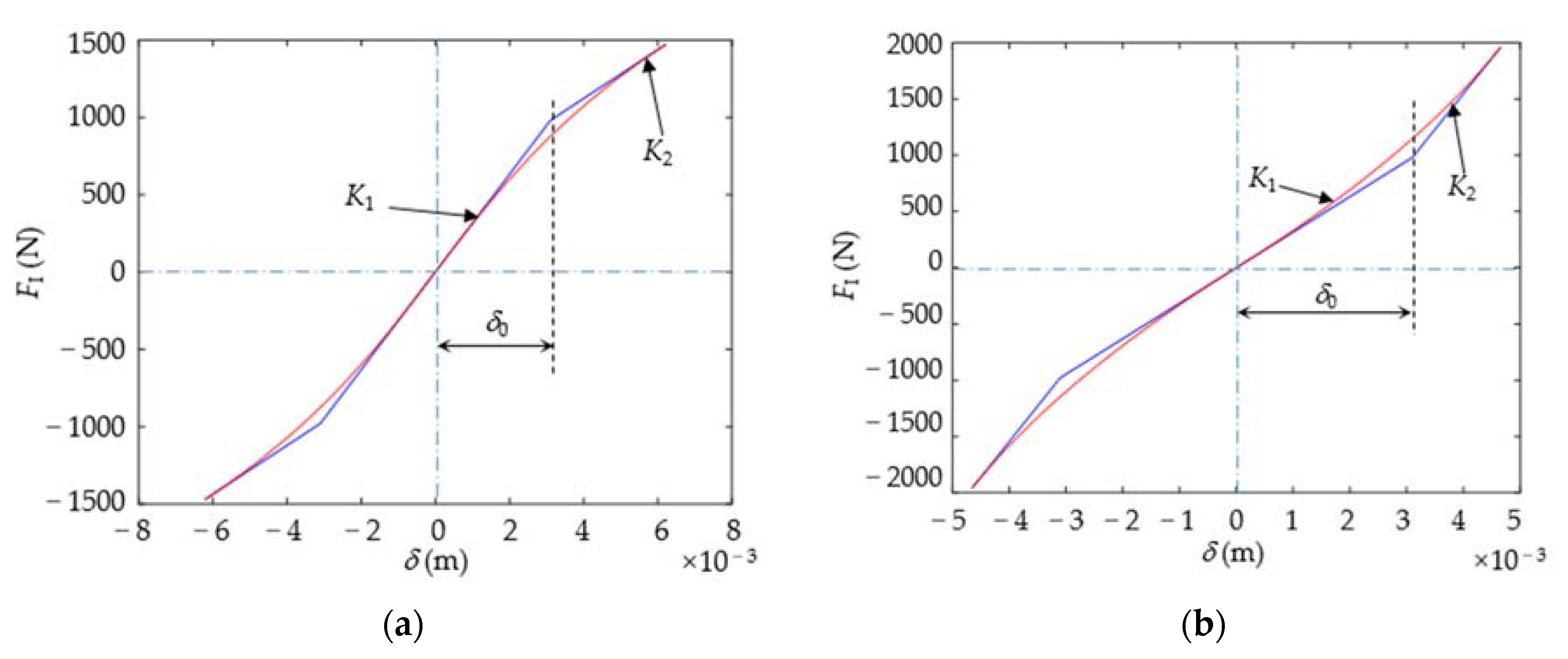
2.3. Expression of Nonlinear Stiffness for Vibration Isolation Supports

In Equations (5) and (8), the constitutive relation of the elastic supports is only expressed in general terms, which can be a linear or nonlinear function. For the nonlinear stiffness characteristics of vibration isolation supports, they are generally classified qualitatively into two categories: softening and hardening characteristics, as shown in Figure 2a,b. The blue curve in Figure 2 indicates the nonlinear stiffness characteristics expressed by a piecewise linear method, where δ₀ is an approximate linear stiffness working interval control parameter, and K₁ and K₂ are approximate stiffness control parameters inside and outside the linear working interval, respectively. In practical problems, the transition from linear to nonlinear generally has a gradual process, rather than a sudden change, and the piecewise curve is not easy to deal with in numerical calculation because of its unsmoothness. So, the piecewise turning function is modified to a smooth transition function, as shown by the red curve in Figure 2.

The softening and hardening characteristics are expressed in this paper as Equations (13) and (14), respectively:

$$\left\{\begin{array}{c}\begin{array}{cc}\delta =\frac{\left|\tau \right|+K_1{c}_1\left[\sqrt[3]{1+{\left(\tau /c_2\right)}^3}-1\right]}{\sqrt{1+K_1^2}}\mathrm{sgn}\left(\tau \right),& F_{\mathrm{I}}=\frac{K_1\left|\tau \right|-c_1\left[\sqrt[3]{1+{\left(\tau /c_2\right)}^3}-1\right]}{\sqrt{1+K_1^2}}\mathrm{sgn}\left(\tau \right)\end{array}\\ \begin{array}{c}{c}_1=\frac{K_1-K_2}{1+K_1{K}_2}{c}_2,\hspace{0.17em}\begin{array}{cc}{c}_2=\sqrt{1+K_1^2}{\delta }_0,& \tau =\left|\tau \right|\mathrm{sgn}\left(\delta \right)\end{array}\end{array}\\ \left[{\left(K_1{c}_1/c_2\right)}^3+1\right]{\left|\tau \right|}^3-3\left(\sqrt{1+K_1^2}\left|\delta \right|+K_1{c}_1\right){\left|\tau \right|}^2+3{\left(\sqrt{1+K_1^2}\left|\delta \right|+K_1{c}_1\right)}^2\left|\tau \right|-{\left(\sqrt{1+K_1^2}\left|\delta \right|+K_1{c}_1\right)}^3+{\left(K_1{c}_1\right)}^3=0\end{array}\right.$$

(13)

where sgn(τ) is the sign function; c₁ and c₂ are shape control parameters determined by K₁, K₂, and δ₀; τ is a parameter variable related to the positive real root |τ| of the polynomial equation.

$$\left\{\begin{array}{c}\begin{array}{cc}\delta =\frac{\left|\tau \right|-K_1{c}_1\left[\sqrt[3]{1+{\left(\tau /c_2\right)}^3}-1\right]}{\sqrt{1+K_1^2}}\mathrm{sgn}\left(\tau \right),& F_{\mathrm{I}}=\frac{K_1\left|\tau \right|+c_1\left[\sqrt[3]{1+{\left(\tau /c_2\right)}^3}-1\right]}{\sqrt{1+K_1^2}}\mathrm{sgn}\left(\tau \right)\end{array}\\ \begin{array}{c}{c}_1=\frac{K_2-K_1}{1+K_1{K}_2}{c}_2,\hspace{0.17em}\begin{array}{cc}{c}_2=\sqrt{1+K_1^2}{\delta }_0,& \tau =\left|\tau \right|\mathrm{sgn}\left(\delta \right)\end{array}\end{array}\\ \left[{\left(K_1{c}_1/c_2\right)}^3-1\right]{\left|\tau \right|}^3+3\left(\sqrt{1+K_1^2}\left|\delta \right|-K_1{c}_1\right){\left|\tau \right|}^2-3{\left(\sqrt{1+K_1^2}\left|\delta \right|-K_1{c}_1\right)}^2\left|\tau \right|+{\left(\sqrt{1+K_1^2}\left|\delta \right|-K_1{c}_1\right)}^3+{\left(K_1{c}_1\right)}^3=0\end{array}\right.$$

(14)

It is assumed that the three groups of vibration isolation supports have the same constitutive relation under the unit A₁, the unit A₂, and the floating raft R. The K₁ of the three groups of vibration isolators are denoted as K_A11 = Re{k₁}, K_A21 = Re{k₂}, and K_R1 = Re{k_R}, respectively, where k₁, k₂, and k_R are the linear complex stiffness. The K₂ of the three groups of isolators (denoted as K_A12, K_A22, and K_R2, respectively) is set as α (stiffness ratio) times K₁, that is, K_A12 = αK_A11, K_A22 = αK_A21, and K_R2 = αK_R1, where α ∈ [0.1, 3.0] (softening characteristic when α < 1.0 and hardening characteristic when α > 1.0). The δ₀ (denoted as δ₁₀, δ₂₀, and δ_R0, respectively) of the three groups of isolators is estimated to be β times their respective static settlement after installation of the units, that is, δ₁₀ = βm₁g/Re{4k₁}, δ₂₀ = βm₂g/Re{4k₂}, and δ_R0 = β(m₁ + m₂ + m_R)g/Re{4k_R}, where β ∈ [0.2, 5.0]. In addition, the structural damping coefficients of the vibration isolators are approximately converted to the equivalent viscous damping coefficients by c₁ = Im{k₁}/ω₁, c₂ = Im{k₂}/ω₁, and c_R = Im{k_R}/ω₁ (where ω₁ is the fundamental frequency of the system).

2.4. Evaluation Index of Vibro-Acoustic Transfer Characteristics for the Nonlinear Coupled System

The transmitted power flow (which refers to the vibrational power flow transferred to the cylindrical shell through the supports under the floating raft in this paper) can reflect the process of vibration energy transfer and conversion into underwater acoustic radiation of the coupled system [34], which can be regarded as a comprehensive reflection of the vibro-acoustic transfer characteristics.

For the coupled system shown in Figure 1, the instantaneous power of the excitation F_y acting on the cylindrical shell by the vibration isolation support is

$$I\left(t\right)=F_{\mathrm{y}}^T·{\dot{w}}_{\mathrm{y}}$$

(15)

The vibrational power flow is the average power of the excitation over a period T = 2π/ω:

$$P_T=\frac{1}{T}{\displaystyle {\int }_0^{T}I\left(t\right)dt}$$

(16)

Similar to this, the time average power is introduced:

$$\overline{I}\left(t\right)=\frac{1}{t}{\displaystyle {\int }_0^{t}I\left(\tau \right)d\tau }$$

(17)

The initial value $\overline{I}\left(t\right)$ can be obtained by the above equation.

$$\overline{I}\left(0\right)=\underset{t\to 0}{\lim }\frac{1}{t}{\displaystyle {\int }_0^{t}I\left(\tau \right)d\tau }=\underset{t\to 0}{\lim }I\left(t\right)=I\left(0\right)=0$$

(18)

The derivative of time t on both sides of Equation (17) is calculated:

$$\dot{\overline{I}}\left(t\right)=-\frac{1}{t^2}{\displaystyle {\int }_0^{t}I\left(\tau \right)d\tau }+\frac{I\left(t\right)}{t}=\frac{-\overline{I}\left(t\right)+I\left(t\right)}{t}$$

(19)

From the above equation, combined with Equations (3), (4), (10), and (15), the initial value $\dot{\overline{I}}\left(t\right)$ can be obtained:

$$\dot{\overline{I}}\left(0\right)=\frac{1}{2}\underset{t\to 0}{\lim }\left({\dot{F}}_{\mathrm{y}}^T·{\dot{w}}_{\mathrm{y}}+F_{\mathrm{y}}^T·{\ddot{w}}_{\mathrm{y}}\right)=\frac{1}{2}\underset{t\to 0}{\lim }\left({\dot{F}}_{\mathrm{y}}^T·2\mathrm{Re}\left\{{\overline{\Phi }}_{\mathrm{C}}^{\mathrm{T}}{S}_{\mathrm{C}}{u}_{\mathrm{C}}\right\}+g^T\left(w_{\mathrm{y}}-w_{\mathrm{b}},{\dot{w}}_{\mathrm{y}}-{\dot{w}}_{\mathrm{b}}\right)·{\ddot{w}}_{\mathrm{y}}\right)=0$$

(20)

where the initial values of the system state variables u_A, u_R, and u_C have been set to be 0 (the system is in a static state).

On the other hand, assuming that the vibration enters the steady state after a certain time t₀ and has a period T, it can be seen from Equation (17) that for any natural number N, the following equation holds:

$$\left(t_0+NT\right)\overline{I}\left(t_0+NT\right)-t_0\overline{I}\left(t_0\right)={\displaystyle {\int }_{t_0}^{t_0+NT}I\left(\tau \right)d\tau }={\displaystyle {\int }_0^{NT}I\left(\tau \right)d\tau }=NT{P}_T$$

(21)

Therefore, the vibration power flow can be calculated by the time average power:

$$P_T=\overline{I}\left(t_0+T\right)+\frac{t_0}{T}\left[\overline{I}\left(t_0+T\right)-\overline{I}\left(t_0\right)\right]$$

(22)

If t₀ is large enough, the system still does not exhibit perfect periodic oscillation. But as long as there is a mathematical expectation in Equation (16), then Equation (22) still holds. At this time, T can be understood as some kind of virtual value related to the excitation period, and P_T still represents the average power level of the excitation. Then, Equation (22) is rewritten as:

$$P_{\mathrm{T}}=\left[\left(T+t_0\right)\overline{I}\left(t_0+T\right)-t_0\overline{I}\left(t_0\right)\right]/T$$

(23)

3. Results and Discussion

Based on the theories in Section 2, the effect of the nonlinear stiffness control parameters of the vibration isolation supports on the low-frequency vibration modes and vibro-acoustic transfer characteristics of the coupled system are analyzed by numerical simulation methods in the following.

To obtain sufficient amplitude for the system to fully demonstrate its nonlinear vibration characteristics, the amplitude of the excitation force applied to the units A₁ and A₂ is set to 500 N. The values of the variable stiffness isolators and system structural parameters involved in the numerical simulations are set as shown in

Table 1. Control parameter settings of variable stiffness vibration isolator.

Control Parameters	Symbols	Units	Values	Remarks
Stiffness control parameters in the approximate linear working interval	KA11	N/m	2.0 × 105
	KA21	N/m	2.7 × 105
	KR1	N/m	8.6 × 105
Stiffness control parameters outside the linear working interval	KA12	N/m	α⋅2.0 × 105	α ∈ [0.1, 3.0] α < 1, softening characteristic α > 1, hardening characteristic
	KA22	N/m	α⋅2.7 × 105
	KR2	N/m	α⋅8.6 × 105
Linear working interval length control parameters	δ10	m	β⋅6.125 × 10−4	β ∈ [0.2, 5.0]
	δ20	m	β⋅6.352 × 10−4
	δR0	m	β⋅6.267 × 10−4
Damping coefficients	c1	kg/s	159.155
	c2	kg/s	214.859
	cR	kg/s	684.366

and

Table 2. System structure parameter settings.

System Structure Parameters		Symbols	Units	Values
Characteristic parameters of the cylindrical shell	Elastic modulus	E	N/m2	2.1 × 1011
	Density	ρ	kg/m3	7.8 × 103
	Poisson’s ratio	μ		0.28
	Dissipation factor	ξ		0.01
	Length, radius, thickness	L, a, d	m	2, 0.4, 0.02
Structure parameters of the units and the raft frame	Mass of the unit A1	m1	kg	50
	Mass of the unit A2	m2	kg	70
	Mass of the raft frame R	mR	kg	100
	Moment of inertia of the unit A1	J1x, J1z	Kg·m2	1, 0.5
	Moment of inertia of the unit A2	J2x, J2z	Kg·m2	1.5, 1
	Moment of inertia of the raft frame R	JRx, JRz	Kg·m2	8.5, 2.5
Linear complex stiffness of the vibration isolation supports	Support stiffness of the unit A1	k1	N/m	2.0 × 105 × (1 + 0.1 j)
	Support stiffness of the unit A2	k2	N/m	2.7 × 105 × (1 + 0.1 j)
	Support stiffness of the raft frame R	kR	N/m	8.6 × 105 × (1 + 0.1 j)
Installation position parameters	Centroid positioning of the unit A1	b1	m	0.25
	Centroid positioning of the unit A2	b2	m	0.25
	Centroid positioning of the raft frame R	LR	m	0.8
	Support spacing of the unit A1	h1x, h1z	m	0.2, 0.3
	Support spacing of the unit A2	h2x, h2z	m	0.2, 0.3
	Support spacing of the raft frame R	Hx, Hz	m	0.35, 0.7

, and other control parameters are shown in Appendix B.

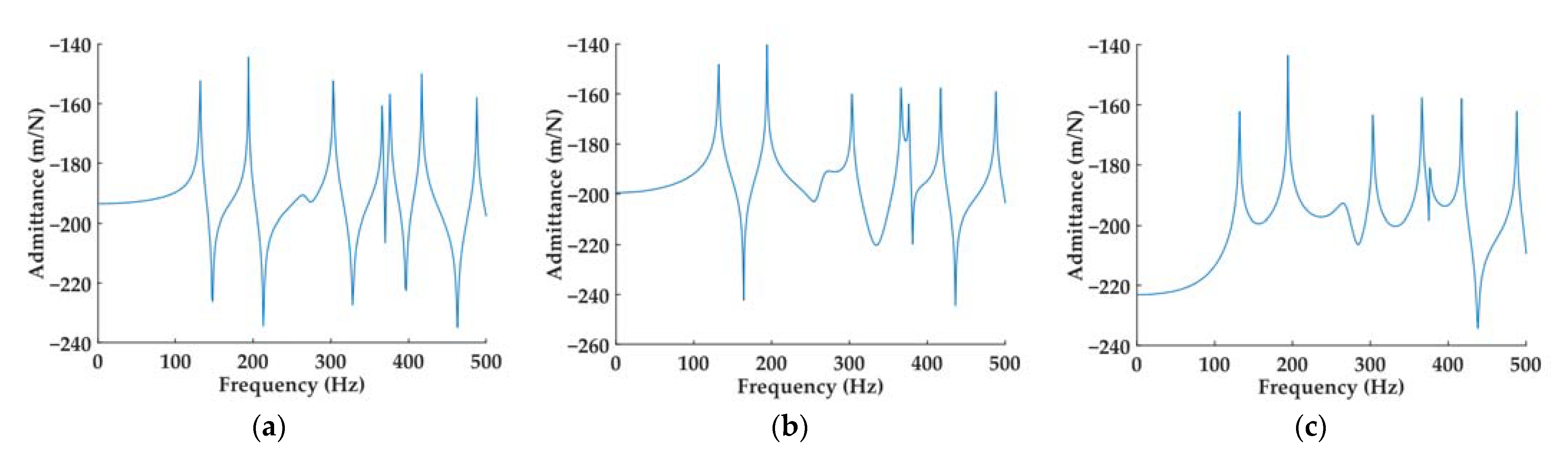
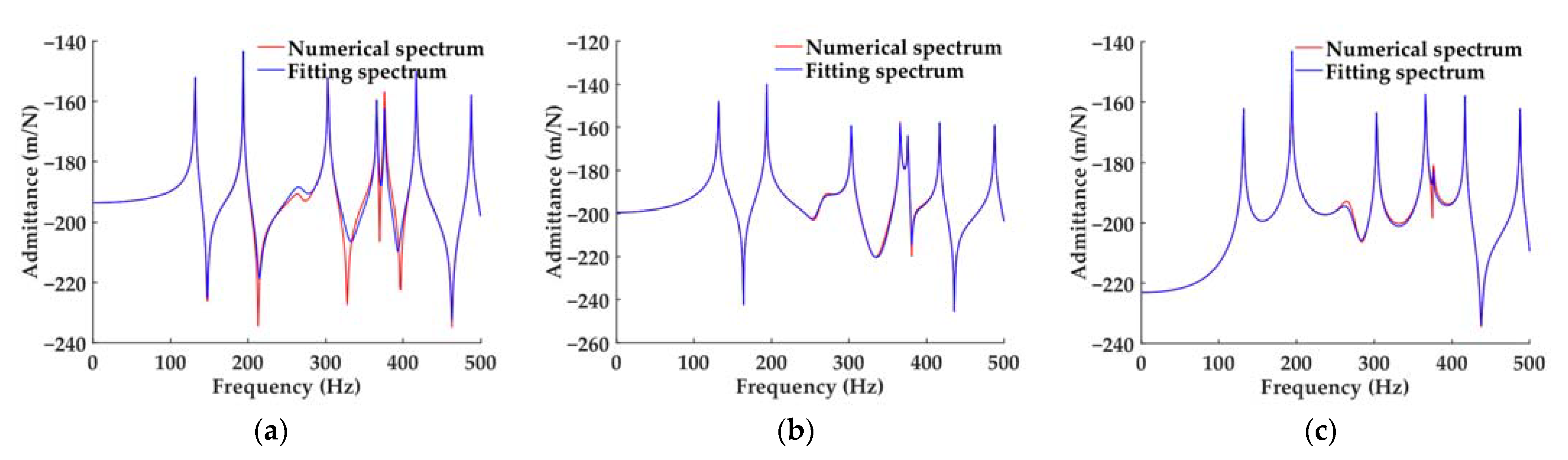
3.1. Modal Parameter Identification for the Cylindrical Shell—Underwater Acoustic Field Coupled Subsystem

Taking the displacement derivative functions H₁₁, H₁₂, and H₁₄ as examples, their fitting spectra obtained from the modal parameter identification method are compared with the numerical spectra obtained by the calculation method in the literature [33], as shown in Figure 3. It can be seen that the fitting results can match well with the original data, and the difference between the two is mainly related to the modal truncation (residual admittance) and the computational error of the original data.

The first 10 orders of poles identified for the cylindrical shell—underwater acoustic field coupled subsystem and their corresponding modal frequencies are listed in

Table 3. The first 10 orders of poles and modal frequencies of the cylindrical shell—underwater acoustic field coupled subsystem.

Orders i	Poles sCi, sCi* *	Modal Frequencies fCi (Hz)
1	−0.366 ± 8.277 × 102 j	131.73
2	−0.574 ± 1.219 × 103 j	194.95
3	−0.660 ± 1.672 × 103 j	266.24
4	−0.924 ± 1.906 × 103 j	303.33
5	−1.246 ± 2.302 × 103 j	366.30
6	−1.753 ± 2.364 × 103 j	376.21
7	−1.307 ± 2.621 × 103 j	417.11
8	−1.586 ± 3.065 × 103 j	487.86
9	−3.624 ± 3.304 × 103 j	525.88
10	−2.863 × 103 ± 1.973 × 103 j	553.34

* The poles s_Ci and s_Ci^* are a pair of conjugate complex numbers.

. The values of the modal parameters ${\overline{\varphi }}_{ij}^{}$ at the support connection points are listed in

Table 4. The values of the modal parameters ${\overline{\varphi }}_{ij}^{}$ at the support connection points.

Orders i	j = 1	j = 2	j = 3	j = 4
i = 1	0.475 − 4.630 j	0.686 − 0.703 j	0.104 − 0.117 j	0.163 − 0.172 j
i = 2	0.462 − 0.429 j	0.601 − 0.647 j	−0.317 + 0.312 j	−0.448 + 0.469 j
i = 3	0.436 − 0.208 j	0.271 − 0.328 j	0.068 − 0.226 j	0.214 − 0.335 j
i = 4	0.510 − 0.529 j	−0.274 + 0.240 j	−0.398 + 0.384 j	0.170 − 0.169 j
i = 5	0.367 − 0.352 j	0.402 − 0.441 j	−0.347 + 0.339 j	−0.453 + 0.479 j
i = 6	0.159 − 0.407 j	−0.342 + 0.117 j	0.412 − 0.031 j	0.006 + 0.032 j
i = 7	0.473 − 0.475 j	−0.218 + 0.218 j	−0.464 + 0.464 j	0.215 − 0.215 j
i = 8	0.357 − 0.356 j	−0.317 + 0.318 j	−0.261 + 0.261 j	0.233 − 0.234 j
i = 9	0.470 − 0.434 j	−0.254 + 0.271 j	−0.361 + 0.357 j	0.248 − 0.270 j
i = 10	0.716 − 0.762 j	0.082 − 0.105 j	−0.244 + 0.233 j	−0.053 + 0.012 j

.

3.2. Effect of Nonlinear Stiffness with Softening Characteristic on the Low-Frequency Vibro-Acoustic Characteristics for the Coupled System

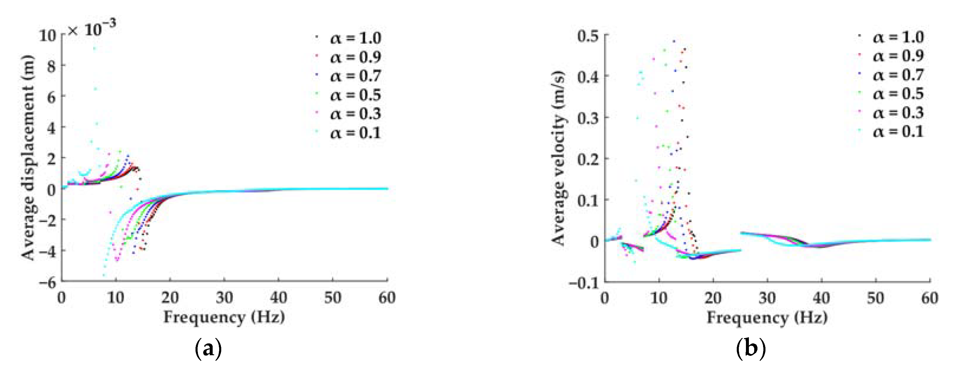
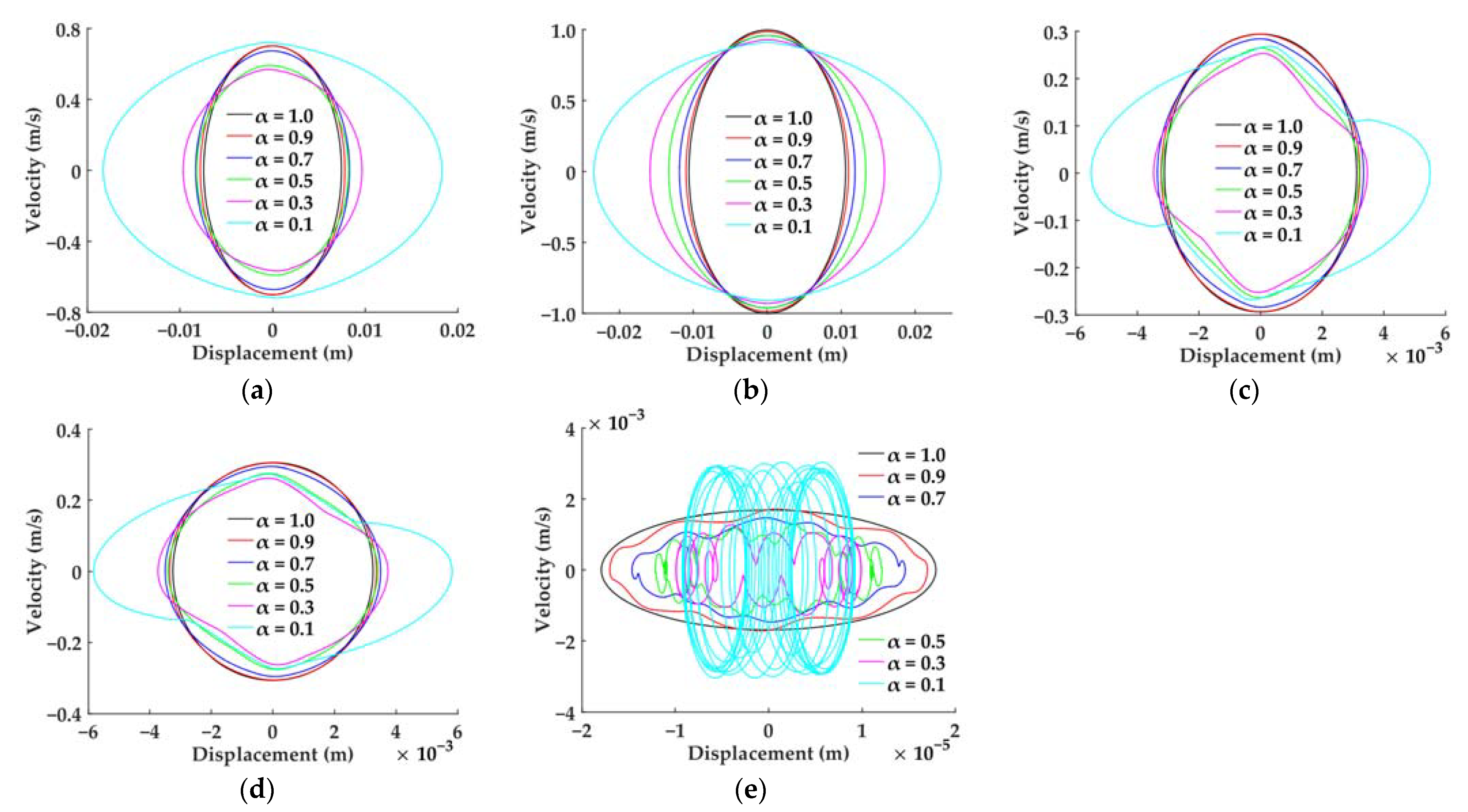
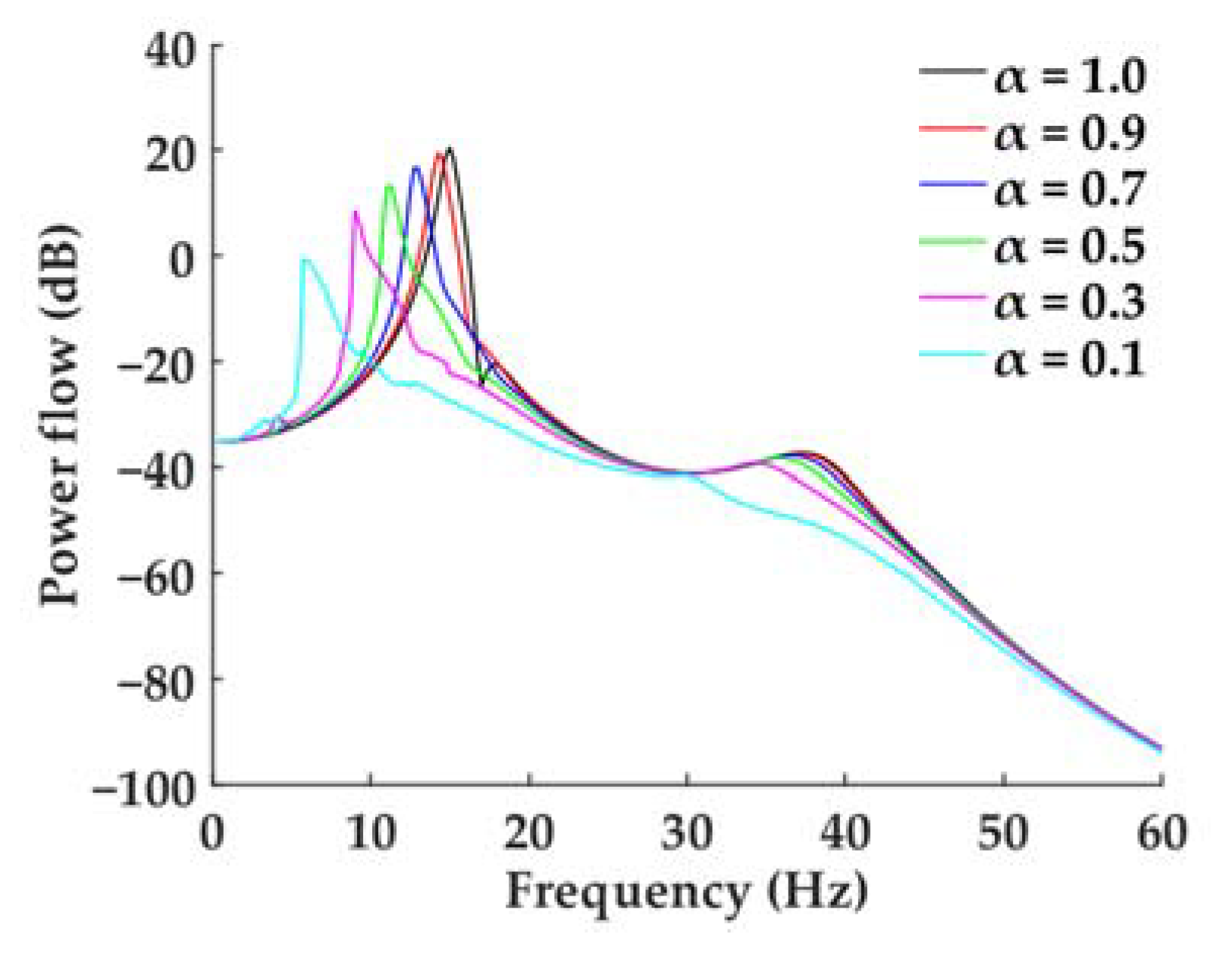
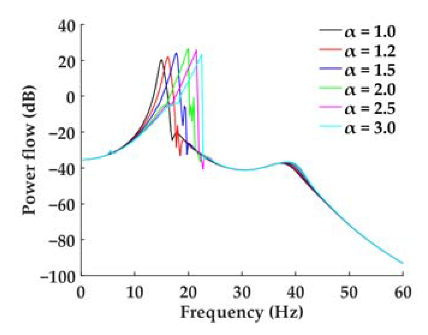
3.2.1. Effect of Stiffness Ratio α

Figure 4 shows the bifurcation diagrams of the average vibration displacement and velocity for the coupled system when β is 1.0 and α is 1.0, 0.9, 0.7, 0.5, 0.3, and 0.1, respectively. Taking α = 0.1 as an example, the discontinuity points near 6.75 Hz in the figure are caused by the system resonating at the natural frequency, while the other discontinuity points are caused by the simulation program setting different steps in different frequency bands to improve the calculation efficiency. The discontinuity points in Figure 4 and in the bifurcation diagram below are the same and will not be explained one by one. It can be seen from Figure 4 that the steady vibration of the coupled system with nonlinear softening stiffness supports is single-periodic motion.

Figure 5 shows the motion phase diagrams of the coupled system corresponding to the resonance frequencies of Figure 4. According to Figure 5a–d, when the softening characteristic is weak (α = 0.9), the units A₁, A₂ and the raft frame all are presented as approximate harmonic vibration modes. As the stiffness ratio decreases, the motion phase diagrams gradually show irregular closed graphics, indicating that the motions of the units A₁, A₂ and the raft frame are still single-periodic, but there are superharmonic components. According to Figure 5e, the vibration form at the connection points of the lower vibration isolators with the cylindrical shell is much more complex than that of the units A₁, A₂ and the raft frame, and the smaller the α, the more complex the vibration form. When α is equal to 0.1, the motion phase diagrams have become disordered or even chaotic. It can also be seen from Figure 5 that in a certain range of stiffness ratio α < 1.0, the resonance displacement amplitudes of the units A₁, A₂ and the raft frame are larger than those of α = 1.0 (linear stiffness), and the smaller the α, the larger the amplitudes. The resonance velocity amplitudes show the opposite trend. In contrast, at the connection points of the lower vibration isolators with the cylindrical shell, the amplitudes of both the resonance displacement and resonance velocity decrease with the decrease in α. But the above law no longer holds when α decreases to a certain extent, as shown in Figure 5e, which is broken when α is equal to 0.1.

In addition, it can be found from Figure 5 that, when the vibration isolation supports have softening stiffness characteristics, the motion laws at the connection points of the upper vibration isolators with units A₁ and A₂ are basically the same, and the motion laws at the connection points of the upper and lower vibration isolators with the raft frame are also basically similar. In fact, through the simulation analysis, it can be seen that the above laws are also established when the vibration isolation supports have hardening stiffness characteristics. Therefore, in the following, only the motion phase diagrams are shown and analyzed at the connection points of the upper vibration isolators with the unit A₁, the lower vibration isolators with the raft frame, and the lower vibration isolators with the cylindrical shell.

Figure 6 shows the transmitted power flow spectrum through the lower vibration isolators input to the cylindrical shell in the coupled system when β is 1.0 and α is 1.0, 0.9, 0.7, 0.5, 0.3, and 0.1, respectively. As can be seen from Figure 6, compared to the linear stiffness, the softening nonlinear characteristic of the support stiffness makes the resonance region of the system shift to lower frequencies, and the resonance peak and the second peak decrease. The smaller α is, the more significant the above effect is.

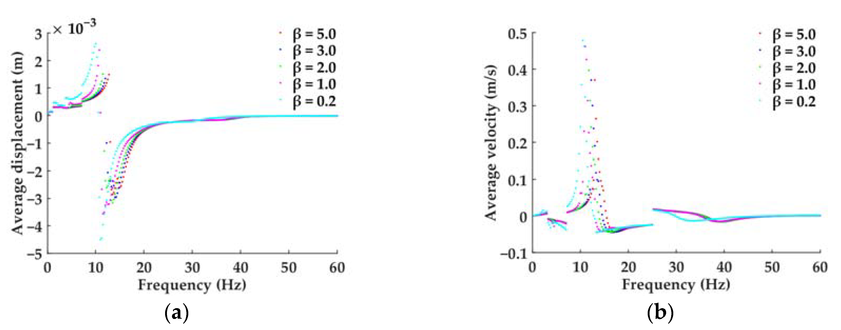
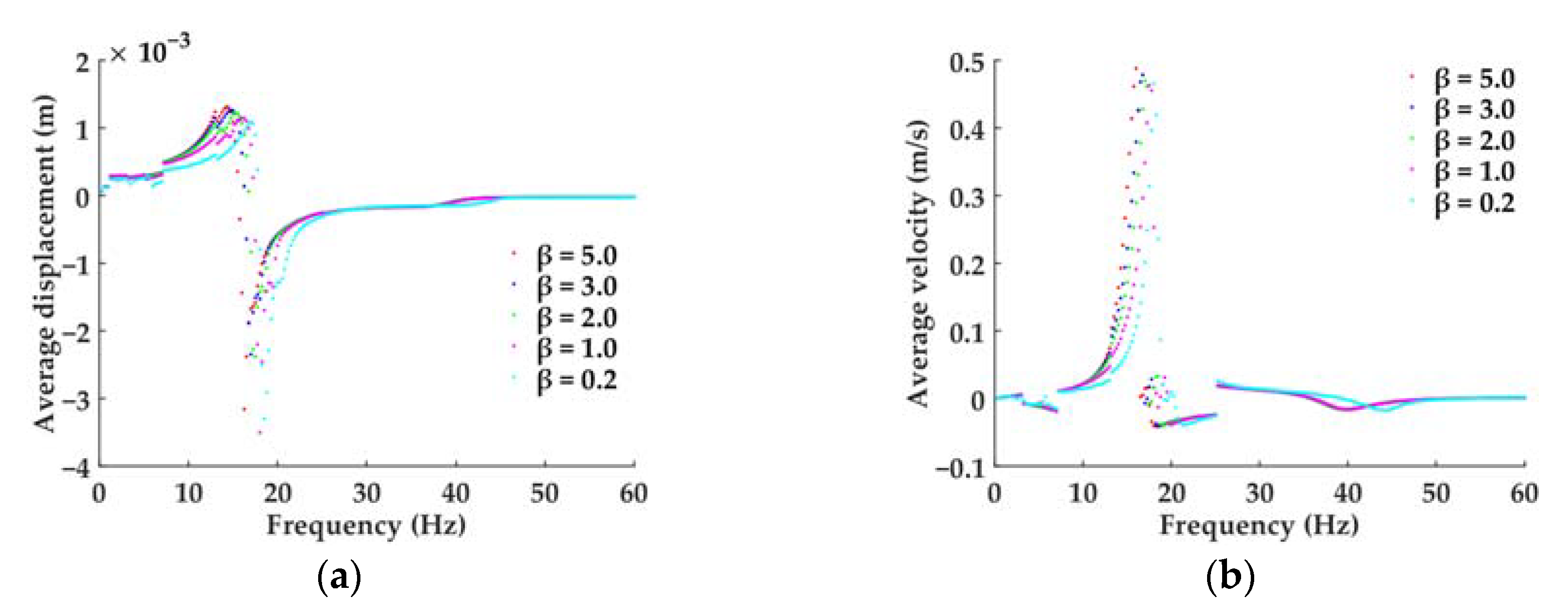
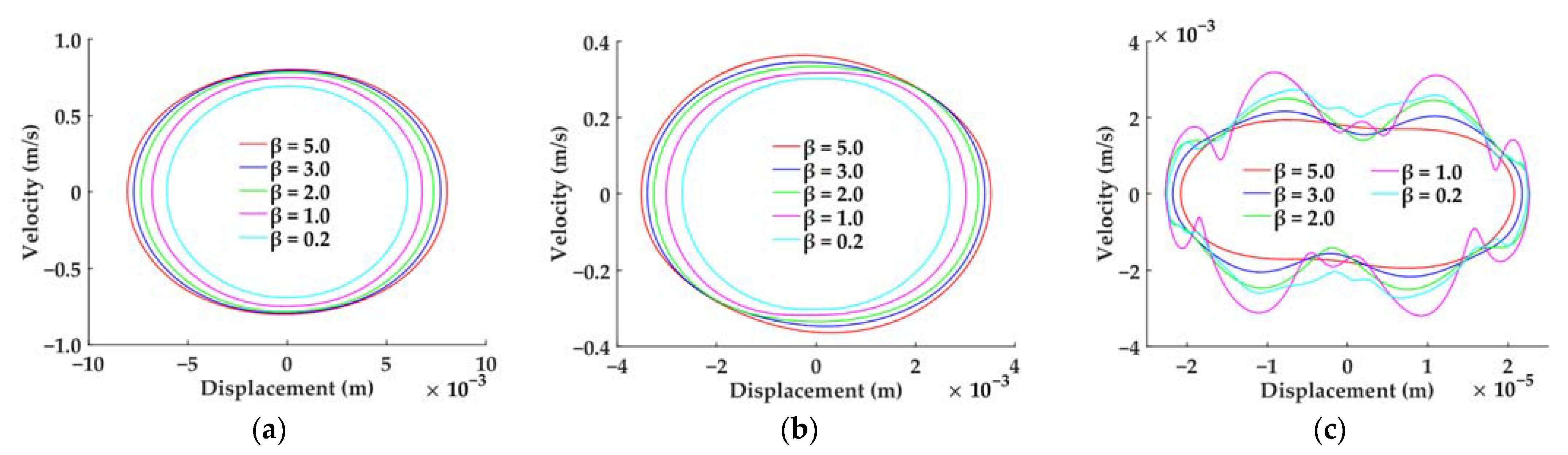
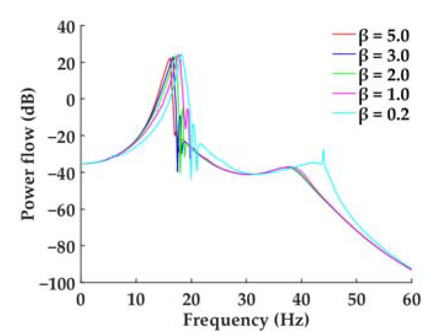
3.2.2. Effect of Approximate Linear Working Interval Length Control Parameter β

Figure 7 shows the bifurcation diagrams of the average vibration displacement and velocity for the coupled system when α is 0.5 and β is 5.0, 3.0, 2.0, 1.0, and 0.2, respectively. Comparing Figure 7 with Figure 4, it can be seen that the two are quite similar, and the steady state vibration of the coupled system is still single-periodic motion.

Figure 8 shows the motion phase diagrams of the coupled system corresponding to the resonance frequencies of Figure 7. Since the stiffness ratio α = 0.5 here has determined that the vibration isolation supports have softening stiffness characteristics, reducing the approximate linear working interval will further strengthen their nonlinear stiffness characteristics. The results are that the amplitudes of the resonance displacement and resonance velocity of the unit, the raft frame, and the connection points of the lower vibration isolators with the cylindrical shell generally tend to increase with the decrease in β. From the perspective of motion form, the motion phase diagram of the unit is approximately a closed ellipse, that is, it is approximately a harmonic vibration. The motion phase diagram of the raft frame is irregular and closed, indicating that it contains strong superharmonic components. The motion phase diagram at the connection points of the lower vibration isolators with the cylindrical shell is relatively complex, indicating that the superharmonic components are complex and strong, and the phase diagram trajectory tends to be messy or even chaotic due to the enhancement of the nonlinear softening characteristic.

Figure 9 shows the transmitted power flow spectrum in the coupled system when α is 0.5 and β is 5.0, 3.0, 2.0, 1.0, and 0.2, respectively. Comparing Figure 9 with Figure 6, it can be seen that the effect of reducing β is similar to that of reducing α. Both of them enhance the nonlinear softening stiffness effect and make the resonance region move to the lower frequency for the coupled system. Reducing α has a more obvious effect on reducing the fundamental frequency of the system and also weakens the resonance sharpness. But reducing β is more effective for reducing the transmitted power flow at higher frequencies after the fundamental frequency. For example, when α is equal to 0.5 and β is equal to 0.2 in Figure 9, the transmitted power flow level is significantly reduced on the band after the fundamental frequency and, especially, the second peak tends to disappear.

3.3. Effect of Nonlinear Stiffness with Hardening Characteristic on the Low-Frequency Vibro-Acoustic Characteristics for the Coupled System

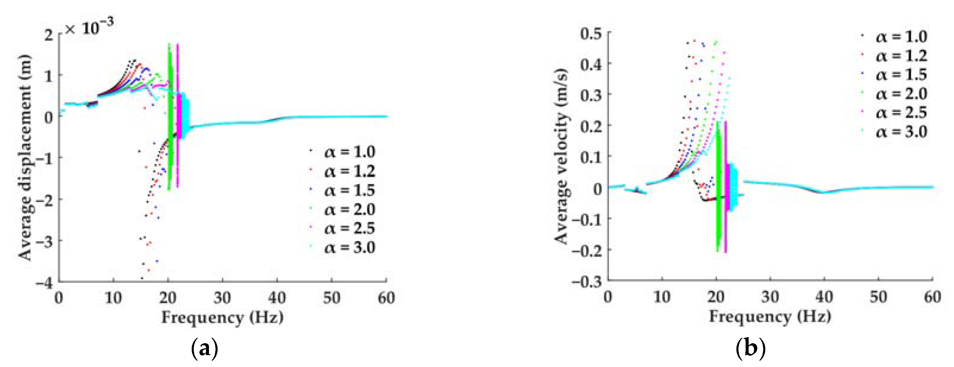
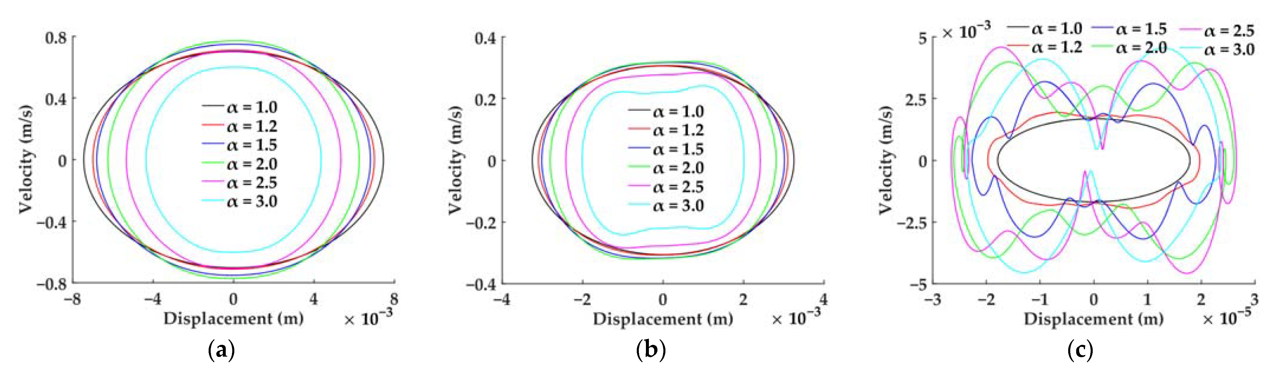
3.3.1. Effect of Stiffness Ratio α

Figure 10 shows the bifurcation diagrams of the average vibration displacement and velocity for the coupled system when β is 1 and α is 1.0, 1.2, 1.5, 2.0, 2.5, and 3.0, respectively. It can be seen that the steady vibration of the coupled system with nonlinear hardening stiffness supports is dominated by single-periodic motion, but when the nonlinear hardening characteristic is enhanced (α = 2.0, 2.5, 3.0), aperiodic motion (quasi-periodic or chaotic) appears in a frequency band after the fundamental frequency resonance region.

Figure 11 shows the motion phase diagrams of the coupled system corresponding to the resonance frequencies of Figure 10. According to Figure 11a, when the hardening characteristic is weak (α = 1.2, 1.5, 2.0), the unit is presented as an approximate harmonic vibration mode. But as the stiffness ratio further increases (α = 2.5, 3.0), the motion phase diagrams gradually become nonelliptical closed graphics, indicating that the motion of the unit is still single-periodic, but there are superharmonic components. According to Figure 5b,c, the motion phase diagrams of the raft and the connection points of the lower vibration isolators with the cylindrical shell are all irregular closed graphics, indicating that their vibration modes are all single-period motion with superharmonics, and the vibration form at the connection points of the lower vibration isolators with the cylindrical shell is particularly complex. Through the calculation and analysis at different frequencies, it can be found that the above vibration modes and laws are universal in the coupled system with hardening characteristic stiffness supports. It can also be seen from Figure 11 that, when stiffness ratio α > 1.0, the resonance displacement amplitudes of the unit and the raft frame are smaller than those of α = 1.0 (linear stiffness), and the larger the α, the smaller the amplitudes. The resonance velocity amplitudes have no consistent change rule. In contrast, at the connection points of the lower vibration isolators with the cylindrical shell, the amplitudes of both the resonance displacement and resonance velocity increase with the increase in α. But they do not conform when α is equal to 3.0, indicating that the above law only holds in a certain range of α > 1.0.

Figure 12 shows the transmitted power flow spectrum in the coupled system when β is 1.0 and α is 1.0, 1.2, 1.5, 2.0, 2.5, and 3.0, respectively. Comparing Figure 12 with Figure 6, it can be seen that the hardening and softening characteristics of the support stiffness have a significantly opposite effect on the transmitted power flow of the coupled system. The hardening nonlinear characteristic of the support stiffness makes the resonance region of the system shift to higher frequencies, and the resonance peak and the second peak increase slightly. The larger α is, the more significant the above effect is.

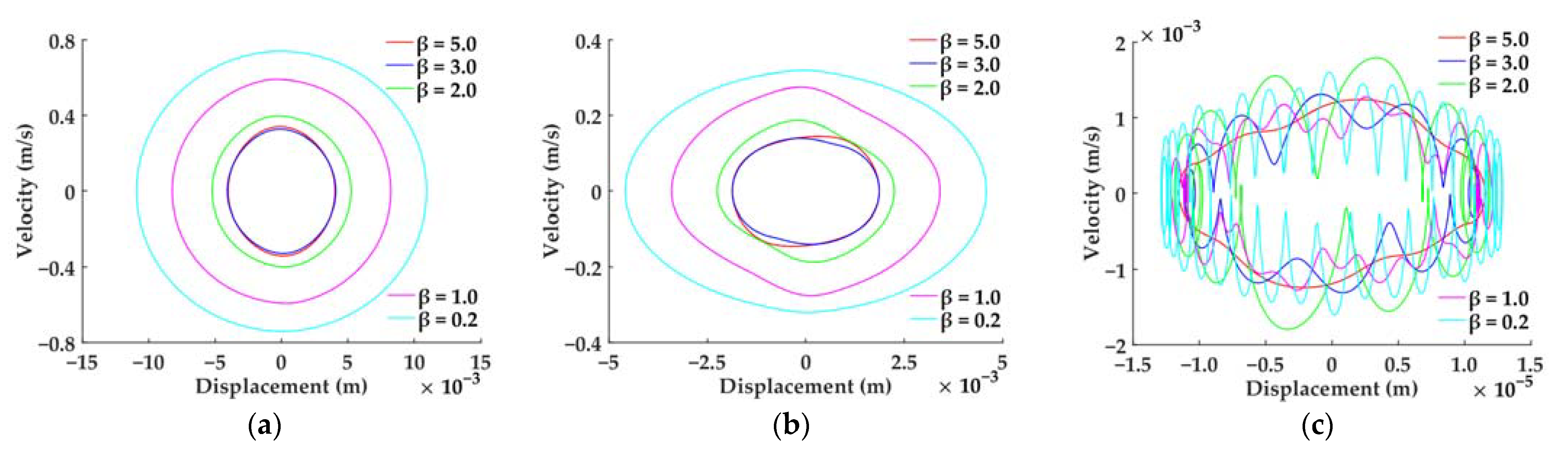
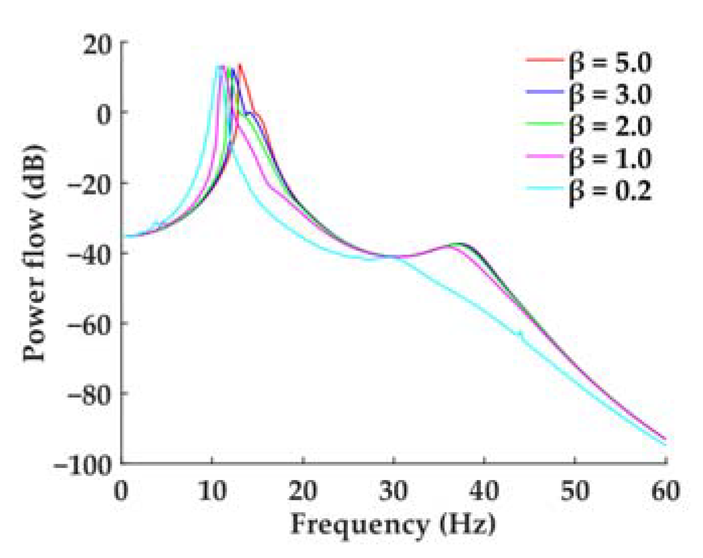
3.3.2. Effect of Approximate Linear Working Interval Length Control Parameter β

Figure 13 shows the bifurcation diagrams of the average vibration displacement and velocity for the coupled system when α is 1.5 and β is 5.0, 3.0, 2.0, 1.0, and 0.2, respectively. Comparing Figure 13 with Figure 10, it can be seen that the two are quite similar, and the steady state vibration of the coupled system is always single-periodic motion when α is equal to 1.5.

Figure 14 shows the motion phase diagrams of the coupled system corresponding to the resonance frequencies of Figure 13. In the case of a given α, the amplitudes of the resonance displacement and resonance velocity of the unit and the raft frame generally tend to decrease with the decrease in β. From the perspective of motion form, the motion phase diagram of the unit is approximately a closed ellipse, that is, it is approximately a harmonic vibration. The motion phase diagram of the raft frame has obvious irregularity, indicating that it contains strong superharmonic components. The motion phase diagram at the connection points of the lower vibration isolators with the cylindrical shell is the most complex, and with the decrease in β, the stability of the phase diagram orbits deteriorates and tends to be messy or even chaotic.

Figure 15 shows the transmitted power flow spectrum in the coupled system when α is 1.5 and β is 5.0, 3.0, 2.0, 1.0, and 0.2, respectively. Comparing Figure 15 with Figure 12, it can be seen that the effect of reducing β is similar to that of increasing α. Both of them enhance the nonlinear hardening stiffness effect and make the resonance region move to the higher frequency for the coupled system. Increasing α leads to a larger range of fundamental frequency variation of the system. But decreasing β extends the effect of nonlinear stiffness characteristics to higher frequencies. For example, when α is equal to 1.5 and β is equal to 0.2 in Figure 15, the effect of the nonlinear hardening characteristics of the vibration isolators extends significantly to higher frequency bands, increasing the transmitted power flow level on the band after the fundamental frequency for the coupled system.

4. Conclusions

The present study was designed to study the effect of support stiffness nonlinearity on the low-frequency vibro-acoustic characteristics for the mechanical equipment—floating raft–cylindrical shell—underwater acoustic field coupled system. Firstly, the state space equations were established for the coupled system containing the vibration isolation supports with nonlinear stiffness characteristics, and in this process, the modal parameter identification method was deduced theoretically and verified by numerical simulation for the cylindrical shell—underwater acoustic field coupled subsystem. Then, the nonlinear stiffness constitutive relation was expressed in general by the softening and hardening characteristics for the vibration isolation supports, and the calculation formulas of the transmitted power flow in the nonlinear vibration isolation system were deduced. Finally, applying the Runge—Kutta method for the dynamics simulation, the effect of the variation of the nonlinear stiffness characteristics parameters on the low-frequency vibration modes and vibro-acoustic transfer characteristics was analyzed and discussed for the coupled system. The main findings are as follows:

• For the coupled system with a nonlinear softening stiffness characteristic of the vibration isolation supports, the steady state vibration mode under harmonic excitation is single-periodic motion, but the superharmonic phenomenon is common. And the smaller the stiffness ratio is, the more superharmonic components are and the more complex the vibration form is. Compared with the linear stiffness case, the softening nonlinear stiffness can reduce the fundamental frequency and decrease the low-frequency vibro-acoustic transmission level within and after the resonance region for the vibration isolation system. And the stronger the softening characteristic is, the more significant the above effect is;
• For the coupled system with a nonlinear hardening stiffness characteristic of the vibration isolation supports, the vibration mode under harmonic excitation is single-periodic motion at most frequencies, and the existence of superharmonics is its main vibration feature. And the larger the stiffness ratio is, the more superharmonic components are and the more complex the vibration form is. In a frequency band slightly higher than the fundamental frequency, it may show a nonperiodic motion mode (quasi-periodic or chaotic). Compared with the linear stiffness case, the hardening nonlinear stiffness can increase the fundamental frequency, broaden the resonance band and slightly raise the low-frequency vibro-acoustic transmission level within and after the resonance region for the vibration isolation system. And the stronger the hardening characteristic is, the more significant the above effect is;
• For the determined nonlinear stiffness ratio, the variation of the length of the approximate linear working interval has no effect on the periodicity of the vibration of the coupled system. For the coupled system with a nonlinear softening stiffness characteristic of the vibration isolation supports, the smaller the length of the approximately linear working interval is, the lower the low-frequency vibro-acoustic transfer level after the fundamental frequency resonance region is; while for the coupled system with a nonlinear hardening stiffness characteristic of the vibration isolation supports, the smaller the length of the approximately linear working interval is, the higher the low-frequency vibro-acoustic transfer level after the fundamental frequency resonance region is.

References

1. Smirnov, V.; Mondrus, V. Comparison of linear and nonlinear vibration isolation system under random excitation. Procedia Eng. 2016, 153, 673–678. [Google Scholar] [CrossRef]
2. Santhosh, B. Dynamics and performance evaluation of an asymmetric nonlinear vibration isolation mechanism. J. Braz. Soc. Mech. Sci. Eng. 2018, 40, 169. [Google Scholar] [CrossRef]
3. Dutta, S.; Chakraborty, G. Performance analysis of nonlinear vibration isolator with magneto-rheological damper. J. Sound Vib. 2014, 333, 5097–5114. [Google Scholar] [CrossRef]
4. Suman, S.; Balaji, P.S.; Selvakumar, K.; Kumaraswamidhas, L.A. Nonlinear vibration control device for a vehicle suspension using negative stiffness mechanism. J. Vib. Eng. Technol. 2021, 9, 957–966. [Google Scholar] [CrossRef]
5. Araki, Y.; Asai, T.; Kimura, K.; Maezawa, K.; Masui, T. Nonlinear vibration isolator with adjustable restoring force. J. Sound Vib. 2013, 332, 6063–6077. [Google Scholar] [CrossRef]
6. Zhao, F.; Ji, J.C.; Ye, K.; Luo, Q. Increase of quasi-zero stiffness region using two pairs of oblique springs. Mech. Syst. Signal Process. 2020, 144, 106975. [Google Scholar] [CrossRef]
7. Zhao, F.; Ji, J.C.; Ye, K.; Luo, Q. An innovative quasi-zero stiffness isolator with three pairs of oblique springs. Int. J. Mech. Sci. 2021, 192, 106093. [Google Scholar] [CrossRef]
8. Ye, K.; Ji, J.C.; Brown, T. Design of a quasi-zero stiffness isolation system for supporting different loads. J. Sound Vib. 2020, 471, 115198. [Google Scholar] [CrossRef]
9. Chang, Y.; Zhou, J.; Wang, K.; Xu, D. A quasi-zero-stiffness dynamic vibration absorber. J. Sound Vib. 2021, 494, 115859. [Google Scholar] [CrossRef]
10. Bouna, H.S.; Nbendjo, B.R.N.; Woafo, P. Isolation performance of a quasi-zero stiffness isolator in vibration isolation of a multi-span continuous beam bridge under pier base vibrating excitation. Nonlinear Dyn. 2020, 100, 1125–1141. [Google Scholar] [CrossRef]
11. Drezet, C.; Kacem, N.; Bouhaddi, N. Design of a nonlinear energy harvester based on high static low dynamic stiffness for low frequency random vibrations. Sens. Actuators A Phys. 2018, 283, 54–64. [Google Scholar] [CrossRef]
12. Lu, Z.; Wu, D.; Ding, H.; Chen, L. Vibration isolation and energy harvesting integrated in a Stewart platform with high static and low dynamic stiffness. Appl. Math. Model. 2021, 89, 249–267. [Google Scholar] [CrossRef]
13. Hao, R.; Lu, Z.; Ding, H.; Chen, L. Orthogonal six-DOFs vibration isolation with tunable high-static-low-dynamic stiffness: Experiment and analysis. Int. J. Mech. Sci. 2022, 222, 107237. [Google Scholar] [CrossRef]
14. Hao, R.; Lu, Z.; Ding, H.; Chen, L. A nonlinear vibration isolator supported on a flexible plate: Analysis and experiment. Nonlinear Dyn. 2022, 108, 941–958. [Google Scholar] [CrossRef]
15. Sun, Y.; Zhou, J.; Thompson, D.; Yuan, T.; Gong, D.; You, T. Design, analysis and experimental validation of high static and low dynamic stiffness mounts based on target force curves. Int. J. Non-Linear Mech. 2020, 126, 103559. [Google Scholar] [CrossRef]
16. Yao, Y.; Li, H.; Li, Y.; Wang, X. Analytical and experimental investigation of a high-static-low-dynamic stiffness isolator with cam-roller-spring mechanism. Int. J. Mech. Sci. 2020, 186, 105888. [Google Scholar] [CrossRef]
17. Chong, X.; Wu, Z.; Li, F. Vibration isolation properties of the nonlinear X-combined structure with a high-static and low-dynamic stiffness: Theory and experiment. Mech. Syst. Signal Process. 2022, 179, 109352. [Google Scholar] [CrossRef]
18. Leutcho, G.D.; Kengne, J. A unique chaotic snap system with a smoothly adjustable symmetry and nonlinearity: Chaos, offset-boosting, antimonotonicity, and coexisting multiple attractors. Chaos Solitons Fractals 2018, 113, 275–293. [Google Scholar] [CrossRef]
19. Yan, B.; Ma, H.; Jian, B.; Wang, K.; Wu, C. Nonlinear dynamics analysis of a bi-state nonlinear vibration isolator with symmetric permanent magnets. Nonlinear Dyn. 2019, 97, 2499–2519. [Google Scholar] [CrossRef]
20. Rahman, Z.A.S.A.; Jasim, B.H. Hidden Dynamics Investigation, Fast Adaptive Synchronization, and Chaos-Based Secure Communication Scheme of a New 3D Fractional-Order Chaotic System. Inventions 2022, 7, 108. [Google Scholar] [CrossRef]
21. Li, Y.; Yi, Y.; Wu, J.; Gu, Y. A novel feature extraction method for ship-radiated noise based on hierarchical refined composite multi-scale dispersion entropy-based Lempel-Ziv complexity. Deep Sea Res. Part I Oceanogr. Res. Pap. 2023, 199, 104111. [Google Scholar] [CrossRef]
22. Karimov, A.; Rybin, V.; Dautov, A.; Karimov, T.; Bobrova, Y.; Butusov, D. Mechanical Chaotic Duffing System with Magnetic Springs. Inventions 2023, 8, 19. [Google Scholar] [CrossRef]
23. Dreau, J.; Magnain, B.; Batailly, A. Multi-element polynomial chaos expansion based on automatic discontinuity detection for nonlinear systems. J. Sound Vib. 2023, 567, 117920. [Google Scholar] [CrossRef]
24. Cassidy, I.L.; Scruggs, J.T. Nonlinear stochastic controllers for power-flow-constrained vibratory energy harvesters. J. Sound Vib. 2013, 332, 3134–3147. [Google Scholar] [CrossRef]
25. Silva, O.M.; Neves, M.M.; Jordan, R.; Lenzi, A. An FEM-based method to evaluate and optimize vibration power flow through a beam-to-plate connection. J. Braz. Soc. Mech. Sci. Eng. 2017, 39, 413–426. [Google Scholar] [CrossRef]
26. Varghese, C.K.; Shankar, K.K. Damage identification using combined transient power flow balance and acceleration matching technique. Struct. Control. Health Monit. 2014, 21, 135–155. [Google Scholar] [CrossRef]
27. Yang, J.; Xiong, Y.; Xing, J. Vibration power flow and force transmission behaviour of a nonlinear isolator mounted on a nonlinear base. Int. J. Mech. Sci. 2016, 115, 238–252. [Google Scholar] [CrossRef]
28. Shi, B.; Yang, J. Quantification of vibration force and power flow transmission between coupled nonlinear oscillators. Int. J. Dyn. Control. 2020, 8, 418–435. [Google Scholar] [CrossRef]
29. Ren, Y.; Chang, S.; Liu, G.; Wu, L.; Wang, H. Vibratory power flow analysis of a gear-housing-foundation coupled system. Shock. Vib. 2018, 2018, 5974759. [Google Scholar] [CrossRef]
30. Zhang, Y.; Zhou, L.; Wang, S.; Yang, T.; Chen, L. Vibration power flow characteristics of the whole-spacecraft with a nonlinear energy sink. J. Low Freq. Noise Vib. Act. Control 2019, 38, 341–351. [Google Scholar] [CrossRef]
31. Xu, D.; Du, J.; Zhao, Y. Flexural vibration and power flow analyses of axially loaded beams with general boundary and non-uniform elastic foundations. Adv. Mech. Eng. 2020, 12, 1687814020921719. [Google Scholar] [CrossRef]
32. Mahapatra, K.; Panigrahi, S.K. Effect of general coupling conditions on the vibration and power flow characteristics of a two-plate built-up plate structure. Mech. Based Des. Struct. Mach. 2021, 49, 841–861. [Google Scholar] [CrossRef]
33. Liu, S.; Huo, R.; Wang, L. Vibroacoustic Transfer Characteristics of Underwater Cylindrical Shells Containing Complex Internal Elastic Coupled Systems. Appl. Sci. 2023, 13, 3994. [Google Scholar] [CrossRef]
34. More, S.; Padmanabhan, C. Power flow based analysis of a floating raft vibration isolation system. Am. Phys. Soc. 2014, 72, 691–708. [Google Scholar]
Figure 1. The model of a mechanical equipment—floating raft—cylindrical shell—underwater acoustic field coupled system: (a) −x direction; (b) z direction; (c) complex coupled system with nonlinear connecting elements.
Inventions 08 00118 g001
Figure 2. Nonlinear stiffness characteristics and their control parameters: (a) softening characteristic; (b) hardening characteristic.
Inventions 08 00118 g002
Figure 3. Comparison of the fitting spectra and the numerical spectra: (a) H11; (b) H12; (c) H14.
Inventions 08 00118 g003
Figure 4. Effect of the strength variation of the nonlinear softening stiffness characteristic on the periodic bifurcation properties for the coupled system (β = 1.0): (a) bifurcation diagram of the average vibration displacement; (b) bifurcation diagram of the average vibration velocity.
Inventions 08 00118 g004
Figure 5. Effect of the strength variation of the nonlinear softening stiffness characteristic on the low-frequency vibration modes for the coupled system (β = 1.0): (a) motion phase diagram at the connection points of the upper vibration isolators with the unit A1; (b) motion phase diagram at the connection points of the upper vibration isolators with the unit A2; (c) motion phase diagram at the connection points of the upper vibration isolators with the raft frame; (d) motion phase diagram at the connection points of the lower vibration isolators with the raft frame; (e) motion phase diagram at the connection points of the lower vibration isolators with the cylindrical shell.
Inventions 08 00118 g005
Figure 6. Effect of the strength variation of the nonlinear softening stiffness characteristic on the vibro-acoustic transfer characteristics for the coupled system (β = 1.0).
Inventions 08 00118 g006
Figure 7. Effect of the length variation of the approximate linear working interval on the periodic bifurcation properties for the coupled system (α = 0.5): (a) bifurcation diagram of the average vibration displacement; (b) bifurcation diagram of the average vibration velocity.
Inventions 08 00118 g007
Figure 8. Effect of the length variation of the approximate linear working interval on the low-frequency vibration modes for the coupled system (α = 0.5): (a) motion phase diagram at the connection points of the upper vibration isolators with the unit A1; (b) motion phase diagram at the connection points of the lower vibration isolators with the raft frame; (c) motion phase diagram at the connection points of the lower vibration isolators with the cylindrical shell.
Inventions 08 00118 g008
Figure 9. Effect of the length variation of the approximate linear working interval on the vibro-acoustic transfer characteristics for the coupled system (α = 0.5).
Inventions 08 00118 g009
Figure 10. Effect of the strength variation of the nonlinear hardening stiffness characteristic on the periodic bifurcation properties for the coupled system (β = 1.0): (a) bifurcation diagram of the average vibration displacement; (b) bifurcation diagram of the average vibration velocity.
Inventions 08 00118 g010
Figure 11. Effect of the strength variation of the nonlinear hardening stiffness characteristic on the low-frequency vibration modes for the coupled system (β = 1.0): (a) motion phase diagram at the connection points of the upper vibration isolators with the unit A1; (b) motion phase diagram at the connection points of the lower vibration isolators with the raft frame; (c) motion phase diagram at the connection points of the lower vibration isolators with the cylindrical shell.
Inventions 08 00118 g011
Figure 12. Effect of the strength variation of the nonlinear hardening stiffness characteristic on the vibro-acoustic transfer characteristics for the coupled system (β = 1.0).
Inventions 08 00118 g012
Figure 13. Effect of the length variation of the approximate linear working interval on the periodic bifurcation properties for the coupled system (α = 1.5): (a) bifurcation diagram of the average vibration displacement; (b) bifurcation diagram of the average vibration velocity.
Inventions 08 00118 g013
Figure 14. Effect of the length variation of the approximate linear working interval on the low-frequency vibration modes for the coupled system (α = 1.5): (a) motion phase diagram at the connection points of the upper vibration isolators with the unit A1; (b) motion phase diagram at the connection points of the lower vibration isolators with the raft frame; (c) motion phase diagram at the connection points of the lower vibration isolators with the cylindrical shell.
Inventions 08 00118 g014
Figure 15. Effect of the length variation of the approximate linear working interval on the vibro-acoustic transfer characteristics for the coupled system (α = 1.5).
Inventions 08 00118 g015