

Flow Instability Control in a Model Swirl-Stabilized Combustor with Central Jet Injection

1
Kutateladze Institute of Thermophysics, 1 Lavrentyev Avenue, 630090 Novosibirsk, Russia
2
Department of Physics, Novosibirsk State University, 1 Pirogov Street, 630090 Novosibirsk, Russia
*
Author to whom correspondence should be addressed.
Inventions 2023, 8(6), 148; https://doi.org/10.3390/inventions8060148
Submission received: 14 September 2023
/
Revised: 31 October 2023
/
Accepted: 7 November 2023
/
Published: 17 November 2023
(This article belongs to the Special Issue Innovative Research and Applications in Hydrodynamics and Flow Control)
Abstract
:Swirling flows often occur in nature and industrial applications. With an increase in swirl intensity, such rotating flows are known to become unstable and undergo a sudden breakdown of the vortex core, resulting in unsteady flow dynamics with intensive pressure fluctuations. In particular, swirling flows are organized in combustion chambers to stabilize the flame around the central recirculation zone, formed due to the vortex core breakdown. However, the impact of large-scale vortex structures, including the precessing vortex core and secondary helical vortices, on unsteady combustion regimes is still unclear. The present paper demonstrates experimentally that for the swirling flow of a model swirl combustor, the injection of a central jet may be used to alter the configuration of coherent flow structures, including helical vortices. In particular, the asymmetric hydrodynamics mode, associated with the precessing vortex core, is suppressed, whereas the symmetrical one becomes dominant. This effect demonstrates the importance of central jet injection to control the dominant mode of flow instability for the design of swirl combustors.
1. Introduction
Rotating or swirling flows are generally realized in combustion chambers of gas turbines for the stabilization of flames. When the rotating flow enters the combustion chamber and expands, the flow at the vortex core decelerates and forms a wake/recirculation zone at the centerline, enclosed by a swirling annular jet. This effect is known as the breakdown of the vortex core [1,2]. A number of large-scale secondary vortex structures are formed in the shear layer between the main annular flow and the central wake zone and are accompanied by smaller-scale eddies and broadband turbulence. The configuration and dynamics of such secondary and primary (the core of the swirling flow) vortices are known to play a key role in turbulent transport and mixing in the near-wake zone. In particular, the vortex core dynamics are often related to slow or strong precession with intensive velocity and pressure fluctuations. In the latter case, the effect is referred to as the precessing vortex core (PVC) [3]. The PVC is known to play an important role in the steady or unsteady operation of gas turbine combustion chambers [4,5,6,7], hydro-turbines [8] and other devices with flow rotation.
The configurations and geometry of real gas turbine combustors are very different. However, in fundamental studies of the features of flow dynamics, mixing and combustion, they are commonly modeled using single (e.g., TURBOMECA design [9,10], PRECCINSTA burner [11]), double (e.g., dual DLR burner [11,12], BIMER device [13]) or even triple [14,15] radial swirlers. Fuel is commonly injected as the central jet/spray, jets between the vanes of a swirler or through a special pre-filmer between two swirlers to organize air-blast atomization [16,17]. The single-swirl models are usually designed to supply fuel gas between the swirler vanes to provide a well-premixed fuel–air mixture at the nozzle of the swirler in order to organize lean-premixed combustion [18]. However, such flames are prone to external perturbation and flow instabilities, thus resulting in thermoacoustic pulsations inside the combustion chamber [11,19,20,21]. Hence, part of the fuel may be supplied as a central jet to organize the pilot flame and stabilize combustion.
However, the central jet also appears to affect the development of hydrodynamic instabilities in the swirling flow. It is well-known that the strong flow pulsations incidental to the PVC in swirling flows are associated with the domination of a global helical instability mode, arising due to the formation of central reverse flow, providing a feedback mechanism. In particular, Midgley and others [9,22] reported that the central jet results in a double-helix vortex structure instead of a spiral PVC for the single-swirler burner based on the Turbomeca design. Later, a similar conclusion was made by Mullyadzhanov et al. [23] for such a burner with combustion based on a large eddy simulation. The present paper reports on a further demonstration of control over the dominant flow instability mode for this burner by injecting a central jet. Turbulent swirling flow is investigated using a combination of stereoscopic particle image velocimetry (PIV) and planar laser-induced fluorescence (PLIF) systems. The measured velocity fluctuation fields are processed using the snapshot proper orthogonal decomposition (POD) method to extract coherent flow structures and analyze the associated vortex structures. Studies of non-reacting flows in combustors are important for better understanding the impact of hydrodynamic instability modes, such as PVC, on momentum and mass transport and to develop strategies for flow control. Moreover, the features of hydrodynamics structure and dynamics of non-reacting flow are important for efficient ignition organization. Numerical simulation of flow and combustion in swirl burners requires adequate modeling of turbulent transport and mixing in the rotating flow, reproduction of emerging large-scale vortex structures and relevant chemical kinetics approximation, accounting for the acoustic modes of the chamber. Therefore, detailed experimental data for non-reacting flows in swirl-stabilized combustors are needed for the first-step validation purposes.
2. Materials and Methods
The measurements are performed for a model gas turbine combustor with a flow swirler and fuel injector based on the Turbomeca design [10]. Detailed information on the configuration of the combustor rig, equipment and data processing routines may be found in a previous study of fuel mixing characteristics [24]. This paper presents only the main parameters of the experimental setup. The flow is organized in an enclosed combustion rig, equipped with flowmeters (Bronkhorst High-Tech) and temperature and pressure transducers, and connected to fuel and air tanks and an exhaust shaft. The rig consists of a plenum section, combustion chamber and cooled exhaust pipe. The swirler is installed inside the plenum section upstream of the combustion chamber. The swirler represents a centerbody with 12 radial vanes with an inclination angle of 30° (see the design in [9]). Fuel is supplied through the holes between the vanes. In addition, fuel can be injected as a central jet from the hole at the tip of the centerbody. The diameter of such a central nozzle is 5.8 mm. The effect of the central jet density on the flow properties was studied in the previous paper [24]. The diameter of the swirler nozzle exit is 37 mm. The Reynolds number of the air flow without a fuel supply corresponds to 3 × 10⁴ with a bulk velocity U0 of 12.8 m/s. This is calculated based on the volume flowrate through the exit of the swirler nozzle.
The measurements of the velocity field in the central longitudinal plane are performed using a stereoscopic PIV system. A sketch of the equipment arrangement relative to the model combustor is shown in Figure 1. The PIV system consists of a pair of 4 Mpix CCD cameras (ImperX Bobcat IGV-B2020, Boca Raton, FL USA), equipped with 105 mm optical lenses (Sigma DG MACRO, Hyogo, Japan) and band-pass optical filters (532 ± 5 nm). Flow tracers, viz., 0.5 μm TiO2 particles, are introduced into the air flow with a fluidized-bed feeder and illuminated in the measurement plane with two light pulses from a double-head Nd:YAG laser (Quantel Ever Green 200, Les Ulis Cedex, France). The duration of the 200 mJ pulses is 6 ns. The laser wavelength is 532 nm. The PIV and PLIF measurements are conducted simultaneously. PLIF is applied for the vapor of acetone admixed to the air flow in the fuel supply line. Acetone is added as a tracer to quantify the turbulent transport and mixing inside the model combustion chamber.
The PLIF system consists of a tunable dye laser (Sirah Precision Scan, Sirah Lasertechnik, Grevenbroich, Germany), which is pumped with a pulsed Nd:YAG laser (QuantaRay) and intensified 5 Mpix sCMOS camera (LaVision, Göttingen, Germany), equipped with a UV-sensitive image intensifier (LaVision IRO Göttingen, Germany), a 100 mm UV lens and an optical band-pass filter (415–455 nm). The pulses of the tunable laser correspond to a wavelength of approximately 283 nm, an energy of 12 mJ, and a duration of about 12 ns. The tunable laser is used to excite the acetone fluorescence in the same cross-section where the PIV measurements are conducted. For this purpose, the PLIF laser beam is converted to a collimated laser sheet with a system of cylindrical and spherical UV lenses. Using photo-bleaching paper, the width and thickness of the laser sheet in the measurement plane are evaluated to be approximately 50 mm and 800 μm, respectively. Each PLIF image is captured within 200 ns between the pair of PIV laser pulses, which are separated by 20 μs.
The PIV and PLIF images are processed using in-house “ActualFlow v.1.18” software. The PIV velocity fields are evaluated using an adaptive cross-correlation algorithm with iterative continuous window shift and refinement (see description in [25]). Examples of the PIV images for two cameras are shown in Figure 2. Both the main annular flow and the central jet are seeded with the tracer particles. The maximal particle shift in the images is approximately 8 pixels. Therefore, the final size of the interrogation area during the interactive cross-correlation of the image pairs for each camera is 32 × 32 pixels. A 50% spatial overlap rate between the interrogation areas is used. A reconstruction of the three-component velocity field in the measurement plane based on two two-component projections to the PIV cameras is performed using the corresponding mapping functions [26] obtained from images of the calibration target, captured prior to the experiments. The mapping function corresponds to a third-order polynomial. The grid spacing of the stereo PIV data is 0.53 mm. For the in-plane velocity components, the accuracy of PIV data is generally accepted as 0.1-pixel (i.e., approximately 1.5% of maximum velocity) accuracy. The accuracy of the normal-to-plane component is expected to be about 3%.
The PLIF images are processed by removing the background signal and correcting the non-uniformity of the laser sheet intensity. In the latter case, an additional CCD camera monitors the light sheet intensity inside a cuvette, filled with a rhodamine 6G solution (see examples in Figure 3). In addition, the attenuation of the PLIF laser sheet in the measurement plane due to absorption is corrected. The PLIF data are back-projected into the measurement plane using the mapping function of the PLIF camera. The obtained data correspond to a regular square grid with a step of approximately 0.5 mm and an actual optical resolution of 1 mm. In total, 1500 snapshots of the PIV and PLIF data are captured simultaneously with an acquisition rate of 5 Hz and used for statistics calculation.
The sets of the measured velocity fluctuation fields u′(x, t) are decomposed into the series (1) of orthonormal spatial functions ϕ(x) (POD modes) and temporal coefficients α(t) based on a singular value decomposition (SVD) procedure (2). In Equation (2), U = [u′(x, t1)…u′(x, tN)], Σ = diag[σ1… σN] and W = [ϕ1(x)…ϕN(x)] are the initial data matrix, matrix of singular values and that of left-singular vectors, respectively. The left-singular vectors in W correspond to the POD modes. V is the matrix of right-singular vectors, where VT consists of the normalized temporal coefficients αq.
In the equations, δij is the Kronecker symbol and I is the identity matrix. M and N are the numbers of the spatial points and temporal snapshots, respectively. In matrix Σ, the singular values are in descending order according to their values, related to the contribution σ2 of each POD mode to the total kinetic energy of the velocity fluctuations in the considered spatial domain. In particular, when flow dynamics are dominated by strong flow pulsations, a low-order model of the phase-averaged flow dynamics can be obtained using the first pair of the most energetic POD modes (3). φ is the phase of the flow pulsations. According to the linear dependence between the matrixes of the POD modes and velocity fluctuation snapshots (4), the PLIF data can be phase-averaged (5) to reveal coherent concentration pulsations. The weight coefficients aqk are the elements of the right-singular vector matrix V. The normalization coefficient in (4) is related to the number of the used snapshots N and appears due to the condition (2). In the present study, 500 snapshots are used for the POD.
3. Results and Discussion
Table 1 presents the flowrates for the considered flows (ln/min according to the normal temperature and pressure standard of NIST). Instead of fuel, a mixture of acetone (with a concentration of 3% by volume) and air is supplied through the central orifice at the tip of the swirler centerbody (as a pilot jet) and through the orifices between the swirler vanes (see Figure 4). The ratio between the mass flowrates of the acetone–air mixture, modeling the gaseous fuel, and air, supplied through the plenum chamber and swirler, corresponds to an equivalence ratio of 0.7 for the case of methane. Three flow cases are considered, where different portions of the acetone–air mixture are injected as the pilot jet, viz., 0%, 10% and 50%.
3.1. Instantenous Snapshots
Figure 5 provides examples of an instantaneous velocity field and a normalized spatial distribution of the local concentration of acetone for the case without pilot jet injection. The velocity components in the measurement plane are shown by (small) arrows, whereas the concentration is indicated with color. Large arrows indicate the approximate locations of large-scale vortex structures, which are present in the inner shear layer between the annular swirling jet and the recirculation zone. The vortex structures are extracted by regions with positive values of a modified Q-criterion [27]. The burner is designed to produce a well-premixed fuel–air mixture at the exit of the swirler nozzle when fuel is injected between the vanes. However, even in the case when 100% acetone is supplied between the vanes, the acetone concentration is not uniform at the entrance of the combustion chamber. Obviously, large-scale vortex structures affect the mixing of acetone inside the chamber, viz., large-scale vortex structures in the inner mixing layer (indicated by the arrows with solid line) are close to observed zones with high acetone concentration.
Figure 6 shows similar examples for the case of a 10% injection. The main difference from the previous case is the high acetone concentration at the exit of the central jet near (x = 0, y = 0). The central jet is directed against the central reverse flow and does not have a potential core due to weak momentum. Thus, the central jet impinges the opposite reverse flow and quickly mixes with it. Figure 7 shows snapshots for the case of a 50% central injection. The arrangement of large-scale vortex structures in the distributions appears to be more symmetrical, and the main flow is associated with the variation in jet opening angle during the propagation of the pairs of large-scale vortex structures in the inner and outer shear layers (marked by solid and dashed arrows, respectively). The central jet also penetrates further into the recirculation zone due to a greater momentum than that for the 10% case. The large-scale vortex structures in the inner and outer mixing layers emerge in pairs, suggesting that they correspond to toroidal vortices or double-helical structures, as predicted by Mullyadzhanov [21].
3.2. Time-Averaged Data
The time-averaged velocity and concentration fields are given in Figure 8. The opening angle of the main annular swirling jet is not sufficiently affected by the central jet (the case of 50% injection is shown), which penetrates into the recirculation zone. The acetone concentration is expectedly high inside the central jet. Figure 9 compares the distributions of the longitudinal and transverse components of the mean velocity near the nozzle exit of the swirler (at y = 3.7 mm) for three considered flow cases. The figure demonstrates that the fuel injection between the vanes has no sufficient impact on the axial velocity distribution at the exit of the annular nozzle of the swirler. The injection of 10% of the acetone–air mixture as the central jet seems to produce a minor effect on the axial flow momentum. However, when 50% of the acetone–air mixture is injected as the central jet, its velocity magnitude is close to that of the annular jet. In addition, the radial velocity profile near x = 0 for the present cross-section suggests that the central jet expands in the radial direction and partially entrains the air inside the reverse flow (see the region near 6 mm < |x| < 10 mm). Thus, the central jet momentum is sufficient to affect the time-averaged flow structure near the exit of the swirler nozzle.
The difference is more pronounced for the Reynolds stresses. Figure 10 and Figure 11 show the mean square deviations of the radial and axial velocity fluctuations <ux′2> and <uy′2>, respectively. Only the kinetic energy of the longitudinal and transverse components of turbulent velocity fluctuations is considered. For the flow region under examination, the shape of the distribution of <uz′2> and the central jet effect are found to be similar to those for <ux′2>. For example, the profiles at y = 3.7 mm are compared in Figure 12. The main observation is that the transverse velocity fluctuations near the center of the nozzle exit (x = 0, y = 0) are suppressed by the central jet. Without this, they reach values of up to 80% of the square of the mean bulk velocity U0. In general, the intensity of the axial velocity fluctuations in the inner shear layer around the reverse flow is also dramatically reduced by the central jet, which forms another conical mixing layer at the jet axis. Thus, whereas the central jet does not strongly affect the mean flow properties, it has a pronounced effect on the anisotropy of velocity fluctuations near the exit of the swirler nozzle. The patterns of large-scale vortex arrangements in the instantaneous snapshots (cf. Figure 5 and Figure 7) also suggest that the properties of the dominant hydrodynamic instability mode are affected by the central jet.
Figure 10 and Figure 11 show the distribution of local axial and radial velocity fluctuations in the swirling annular jet (x = 8.5 mm, y = 3.7 mm) and near the centerline (x ≈ 1.1 mm, y = 3.7 mm). If the influence of the central jet is insufficient for the region of the main swirling flow, the distributions of the velocity fluctuations become very different for the centerline region. In all cases, the local distributions of velocity fluctuations are far from a Gaussian shape, which is typical for normally distributed random variables. As demonstrated in the next subsection, this is due to intensive coherent velocity fluctuations in the flow, produced by the motion of large-scale vortex structures. For the near-axis region, the effect of the central jet is very strong, which results in narrow bell-shaped distributions. For the axial velocity component, the distribution is accompanied by less-probable small values of axial velocity, indicating that the central jet is sometimes suppressed by reverse flow at the centerline.
Figure 13 shows the effect of the central jet on the intensity of acetone concentration fluctuations. The local fluctuation probabilities are also analyzed near the centerline and in the region of the annular swirling jet. The concentration values are normalized by the maximal observed concentration values at the exit of the central jet. In the region of the main annular flow, the effect of the central jet injection (the 50% case is shown) is minor. It is noteworthy, that without the central jet, the distribution of acetone concentration fluctuations in the shown locations are quite similar. This is in agreement with the previous observation that the fuel injection between the swirler vanes does not provide complete mixing. The injection of 50% acetone through the central jet results in a greater average concentration and also in a greater width of the distribution. Thus, the central jet injection does not strongly affect the mean velocity distribution in the flow and has only a local effect on the fuel concentration fluctuations in the region close to the jet core. However, the intensities of the longitudinal and transverse velocity fluctuations are affected dramatically in the considered flow region.
3.3. Coherent Fluctuations
To reveal coherent flow structures, the velocity snapshots are processed using the POD method. Figure 14 provides the distribution of the kinetic energy of velocity fluctuations related to different modes for the considered three flow cases. The energy is evaluated as σk2. As can be seen, in all cases, there are two dominant modes that are typical for the flow. The cases without and with a 50% injection are associated with approximately 20% of the turbulent kinetic energy for the considered spatial domain. For the case of 10%, the content is insignificant, viz., 15%. The inset in Figure 12 contains the values of the temporal coefficients of the first two POD modes α1(t) and α2(t). Apparently, for the case without injection and the case of a 50% injection, the values are scattered around a Lissajous figure circle, indicating that these two modes are statistically correlated. In these cases, the flow dynamics can be represented by the low-order model (3). For the case of a 10% injection, the scattering is considerably greater.
Figure 15 shows distributions of the first four POD modes for the case without injection. Two in-plane components of the POD modes are shown by vectors, whereas the color corresponds to the phase-averaged fluctuations in acetone concentration. These fluctuation amplitudes reach up to 4% of C0. The first two POD modes are related to intensive velocity and concentration fluctuations in the inner and outer mixing layers. The distributions appear to be almost anti-symmetric relative to the centerline. Therefore, they are suggested to correspond to the PVC mode with intensive flow fluctuations. The third and fourth modes are associated with larger but less intensive velocity and concentration fluctuations.
Figure 16 shows the distribution of the first four POD modes for the case of a 10% central jet injection. The first two modes also manifest antisymmetric properties of velocity and concentration fluctuations even in the region of the central jet. Therefore, it is concluded that the PVC still determines the flow dynamics and the turbulent transport of acetone near the nozzle exit. However, the third and fourth POD modes also exhibit quite a high magnitude of velocity and concentration fluctuations. There, the turbulent kinetic energy content is about 7% in comparison with 15% for the first two modes. In addition, the fourth POD mode clearly demonstrates the nearly symmetric mode of velocity and concentration fluctuations. Thus, the injection of a weak central jet promotes another hydrodynamic instability mode, corresponding to an even azimuthal mode.
Figure 17 shows the first four POD modes for the case of a 50% injection. It is clear that in this case, the symmetrical mode is dominant and corresponds to the first most energetic POD modes. Antisymmetric coherent velocity and concentration fluctuations are visible in the third POD mode, but the energy content is much smaller for this mode (3.2%). Currently, there is evidence of PVC for this case. Thus, the injection of the central jet allows altering the properties of the dominant instability mode and, in particular, replacing an antisymmetric (odd) mode with one having reflective symmetry relative to the centerline (even azimuthal mode). This approach may be used to suppress thermoacoustic pulsations in combustion chambers.
3.4. Stochastic Fluctuations
When the flow dynamics are dominated by coherent flow pulsations, the velocity fluctuations can be decomposed into coherent and stochastic parts u′ = û+u″ [28]. The use of POD allows for separating the contribution of the stochastic and coherent velocity fluctuations to the total Reynolds stresses and Reynolds fluxes:
Figure 18 compares the intensity of stochastic velocity fluctuations for the radial and axial velocity components. The difference between the distributions and magnitude is not as substantial as for the total fluctuations, as shown in Figure 10 and Figure 11. The effect of the central jet injection on the entire flow is also rather minor, except for the region around the central jet. Thus, the central jet affects mainly the properties of coherent velocity fluctuations, which manifest strong anisotropy of the velocity fluctuations. Figure 19 and Figure 20 also compare the effect of the central jet on the Reynolds stress and flux, respectively, for the total fluctuations and the stochastic part. The central jet strongly affects the entire distribution of the total Reynolds shear stress, whereas, for the stochastic part, the effect is mainly near the central jet. The contribution of the coherent part to the total turbulent shear stress is found to be above 65% near the exit of the swirler nozzle for the cases without and with the central jet injection. The contribution is found to be even stronger in the case of the radial turbulent flux plotted in Figure 20. Only near the core of the central jet (for the case of 50% supply) do stochastic fluctuations provide sufficient turbulent transport of the admixture. Thus, it is concluded that for all considered flow cases, coherent velocity fluctuations play a dominant role in the turbulent mass and momentum transport in the inner mixing layer around the central recirculation zone. The central jet strongly affects the turbulent transport in the inner mixing layer by altering the properties of large-scale coherent structures, whereas its effect inside the recirculation zone is minor.
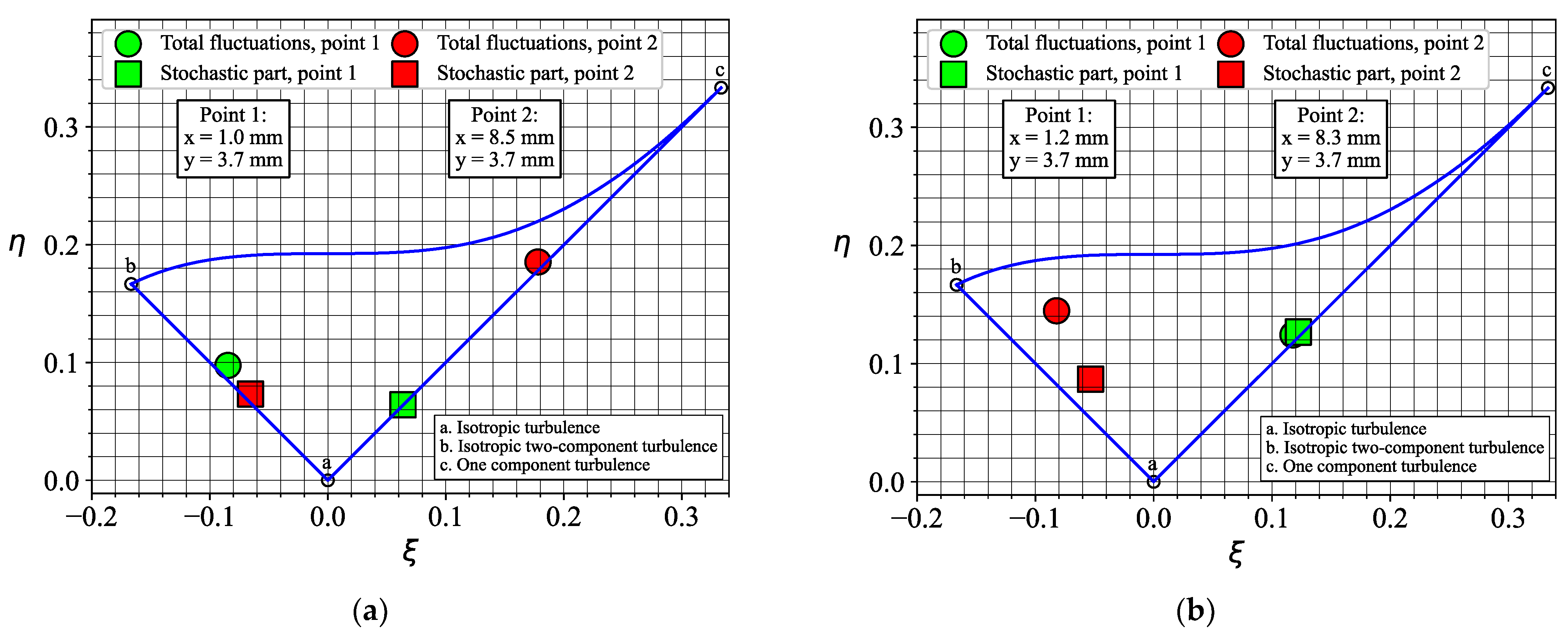
Figure 21 compares linearized anisotropy invariant maps of the velocity fluctuations in the inner mixing layer around the central recirculation zone (x = 8.5 mm, y = 3.7 mm) and near the flow axis (x ≈ 1.1 mm, y = 3.7 mm). The maps correspond to the local values of modified invariants η and ξ defined by (8), where II and III are the invariants (9) of the characteristic equation for the anisotropy tensor bij (10) for the Reynolds shear stress [29]. The data are shown for the total or stochastic velocity fluctuations. In the latter case (square symbols), the effect of the central jet is minor, whereas, for the total fluctuations, the effect is clearly visible. With and without the central jet, the stochastic fluctuations near the flow axis and in the inner shear layer manifest properties of axisymmetric turbulence, with one component being considerably higher and lower in comparison to the other two, respectively. For the total velocity fluctuations, the injection of the central jet leads to the switching between the properties of the axial symmetry near the flow axis and the inner mixing layer.
4. Conclusions
The present paper reports on the PIV and PLIF measurements of flow structure and turbulent fluctuations in a model swirl-stabilized combustor with a two-zone swirl burner based on Turbomeca geometry. The swirler provides fuel injection in the form of a central jet to organize a pilot flame, and upstream the exit of the nozzle between the swirler vanes, to ensure the supply of a well-premixed fuel. PIV and PLIF measurements demonstrate that when gas is supplied between the vanes, its concentration at the entrance to the combustion chamber is still considerably nonuniform and fluctuates inside the chamber due to the presence of a large-scale vortex structure. The analysis of the coherent velocity fluctuations with POD suggests that the vortex structure in the inner mixing layer corresponds to the spiral PVC. Injecting part (10%) of the fuel gas as a central control jet contributes to another instability mode that exhibits reflection symmetry relative to the geometric axis. When half of the fuel is supplied through the central jet, the PVC mode appears to be suppressed, and the flow dynamics are driven by a symmetrical mode, related to either toroidal or double-helix vortex structures. Thus, the central jet injection does not have a strong influence on the mean velocity distribution in the flow, only locally affecting the fuel concentration fluctuation in the region close to the jet core. However, the intensities of the longitudinal and transverse velocity fluctuations and the properties of the dominant hydrodynamic instability mode are affected dramatically in the near-nozzle flow region. Moreover, for all considered flow cases, it is found that the coherent velocity fluctuations play a dominant role in the turbulent mass and momentum transport in the inner mixing layer around the central recirculation zone. Thus, the central jet strongly affects turbulent transport in the inner mixing layer by altering the properties of large-scale coherent structures, whereas its effect inside the recirculation zone is minor. Therefore, the central jet injection may be used to control the dominant mode of flow instability and, in particular, to suppress thermo-acoustic instabilities during combustion.
Author Contributions
Conceptualization, V.D. and L.C.; methodology, D.S.; data processing, D.S. and A.S.; data acquisition, D.S. and A.S.; writing—original draft preparation, V.D. and L.C.; writing—review and editing, V.D.; visualization, A.S.; supervision, V.D.; project administration, L.C.; funding acquisition, L.C. All authors have read and agreed to the published version of the manuscript.
Funding
This research was supported by the Ministry of Science and Higher Education of the Russian Federation, agreement No. 075-15-2020-806.
Data Availability Statement
The data that support the findings of this study are available from the corresponding author upon reasonable request.
Acknowledgments
The authors are grateful to Roman Tolstoguzov for assistance during the experiments.
Conflicts of Interest
The authors declare no conflict of interest.
References
- Billant, P.; Chomaz, J.M.; Huerre, P. Experimental study of vortex breakdown in swirling jets. J. Fluid Mech. 1998, 376, 183–219. [Google Scholar] [CrossRef]
- Lucca-Negro, O.; O’doherty, T. Vortex breakdown: A review. Prog. Energy Combust. Sci. 2001, 27, 431–481. [Google Scholar] [CrossRef]
- Syred, N. A review of oscillation mechanisms and the role of the precessing vortex core (PVC) in swirl combustion systems. Prog. Energy Combust. Sci. 2006, 32, 93–161. [Google Scholar] [CrossRef]
- Stöhr, M.; Arndt, C.M.; Meier, W. Transient effects of fuel–air mixing in a partially-premixed turbulent swirl flame. Proc. Combust. Inst. 2015, 35, 3327–3335. [Google Scholar] [CrossRef]
- Stöhr, M.; Sadanandan, R.; Meier, W. Experimental study of unsteady flame structures of an oscillating swirl flame in a gas turbine model combustor. Proc. Combust. Inst. 2009, 32, 2925–2932. [Google Scholar] [CrossRef]
- Boxx, I.; Stöhr, M.; Carter, C.; Meier, W. Temporally resolved planar measurements of transient phenomena in a partially pre-mixed swirl flame in a gas turbine model combustor. Combust. Flame 2010, 157, 1510–1525. [Google Scholar] [CrossRef]
- Oberleithner, K.; Paschereit, C.O.; Seele, R.; Wygnanski, I. Formation of turbulent vortex breakdown: Intermittency, criticality, and global instability. AIAA J. 2012, 50, 1437–1452. [Google Scholar] [CrossRef]
- Shtork, S.; Suslov, D.; Skripkin, S.; Litvinov, I.; Gorelikov, E. An Overview of Active Control Techniques for Vortex Rope Mitigation in Hydraulic Turbines. Energies 2023, 16, 5131. [Google Scholar] [CrossRef]
- Midgley, K.; Spencer, A.; McGuirk, J.J. Unsteady Flow Structures in Radial Swirler Fed Fuel Injectors. ASME J. Eng. Gas Turbines Power 2005, 127, 755–764. [Google Scholar] [CrossRef]
- Janus, B.; Dreizler, A.; Janicka, J. Experimental study on stabilization of lifted swirl flames in a model GT combustor. Flow Turbul. Combust. 2005, 75, 293–315. [Google Scholar] [CrossRef]
- Meier, W.; Weigand, P.; Duan, X.R.; Giezendanner-Thoben, R. Detailed characterization of the dynamics of thermoacoustic pulsations in a lean premixed swirl flame. Combust. Flame 2007, 150, 2–26. [Google Scholar] [CrossRef]
- Meier, W.; Duan, X.R.; Weigand, P. Investigation of swirl flames in a gas turbine model combustor II. Turbulence-chemistry interactions. Combust. Flame 2006, 144, 225–236. [Google Scholar] [CrossRef]
- Renaud, A.; Ducruix, S.; Scouflaire, P.; Zimmer, L. Flame shape transition in a swirl stabilised liquid fueled burner. Proc. Combust. Inst. 2015, 35, 3365–3372. [Google Scholar] [CrossRef]
- Li, G.; Gutmark, E.J. Geometry effects on the flow field and spectral characteristics of a triple annular swirler. In Proceedings of the ASME Turbo Expo, Power for Land, See and Air, Atlanta, GA, USA, 16–19 June 2003; 2003. [Google Scholar] [CrossRef]
- Vashahi, F.; Lee, J. Effects of the Interaction Point of Adjacent Swirlers on Swirling Flow Using POD Analysis in a Triple Swirler Configuration. J. Eng. Gas Turbines Power 2019, 141, 0610113. [Google Scholar] [CrossRef]
- Wehr, L.; Meier, W.; Kutne, P.; Hassa, C. Single-pulse 1D laser Raman scattering applied in a gas turbine model combustor at elevated pressure. Proc. Combust. Inst. 2007, 31, 3099–3106. [Google Scholar] [CrossRef]
- Stöhr, M.; Sadanandan, R.; Meier, W. Phase-resolved characterization of vortex–flame interaction in a turbulent swirl flame. Exp. Fluids 2011, 51, 1153–1167. [Google Scholar] [CrossRef]
- Dunn-Rankin, D. Lean Combustion. Technology and Control; Elsevier: Oxford, UK, 2008. [Google Scholar]
- Lieuwen, T.; Torres, H.; Johnson, C.; Zinn, B.T. A mechanism of combustion instability in lean premixed gas turbine combustors. J. Eng. Gas Turbines Power 2001, 123, 182–189. [Google Scholar] [CrossRef]
- Candel, S.; Durox, D.; Schuller, T.; Bourgouin, J.-F.; Moeck, J.P. Dynamics of swirling flames. Ann. Rev. Fluid Mech. 2014, 46, 147–173. [Google Scholar] [CrossRef]
- Lieuwen, T.C. Unsteady Combustor Physics; Cambridge University Press: Cambridge, UK, 2021. [Google Scholar]
- Spencer, A.; McGuirk, J.; Midgley, K. Vortex breakdown in swirling fuel injector flows. J. Eng. Gas Turbines Power 2008, 130, 021503. [Google Scholar] [CrossRef]
- Palkin, E.V.; Hrebtov, M.Y.; Slastnaya, D.A.; Mullyadzhanov, R.I.; Vervisch, L.; Sharaborin, D.K.; Lobasov, A.S.; Dulin, V.M. Influence of a Central Jet on Isothermal and Reacting Swirling Flow in a Model Combustion Chamber. Energies 2022, 15, 1615. [Google Scholar] [CrossRef]
- Sharaborin, D.K.; Savitskii, A.G.; Bakharev, G.Y.; Lobasov, A.S.; Chikishev, L.M.; Dulin, V.M. PIV/PLIF investigation of unsteady turbulent flow and mixing behind a model gas turbine combustor. Exp. Fluids 2021, 62, 96. [Google Scholar] [CrossRef]
- Scarano, F. Iterative image deformation methods in PIV. Meas. Sci. Technol. 2001, 13, R1–R19. [Google Scholar] [CrossRef]
- Soloff, S.M.; Adrian, R.J.; Liu, Z.-C. Distortion compensation for generalized stereoscopic particle image velocimetry. Meas. Sci. Technol. 1997, 8, 1441–1454. [Google Scholar] [CrossRef]
- Lobasov, A.S.; Alekseenko, S.V.; Markovich, D.M.; Dulin, V.M. Mass and momentum transport in the near field of swirling turbulent jets. Effect of swirl rate. Int. J. Heat Fluid Flow 2020, 83, 108539. [Google Scholar] [CrossRef]
- Hussain, A.K.M.F.; Reynolds, W.C. The mechanics of an organized wave in turbulent shear flow. J. Fluid Mech. 1970, 41, 241–258. [Google Scholar] [CrossRef]
- Choi, K.-S.; Lumley, J.L. The return to isotropy of homogeneous turbulence. J. Fluid Mech. 2001, 436, 59–84. [Google Scholar] [CrossRef]
Figure 1.
Sketch of the experimental setup and combustion chamber design.

Figure 2.
Examples of stereoscopic PIV images captured with two separate cameras.

Figure 3.
Examples of PLIF images captured in the measurement area (left) and in the calibration cuvette (right).
Figure 3.
Examples of PLIF images captured in the measurement area (left) and in the calibration cuvette (right).

Figure 4.
Design of the swirler with changeable radial vanes.

Figure 5.
Examples of the instantaneous flow velocity and model fuel concentration for the case without central jet injection. The snapshots are captured in the central x0y plane.
Figure 5.
Examples of the instantaneous flow velocity and model fuel concentration for the case without central jet injection. The snapshots are captured in the central x0y plane.
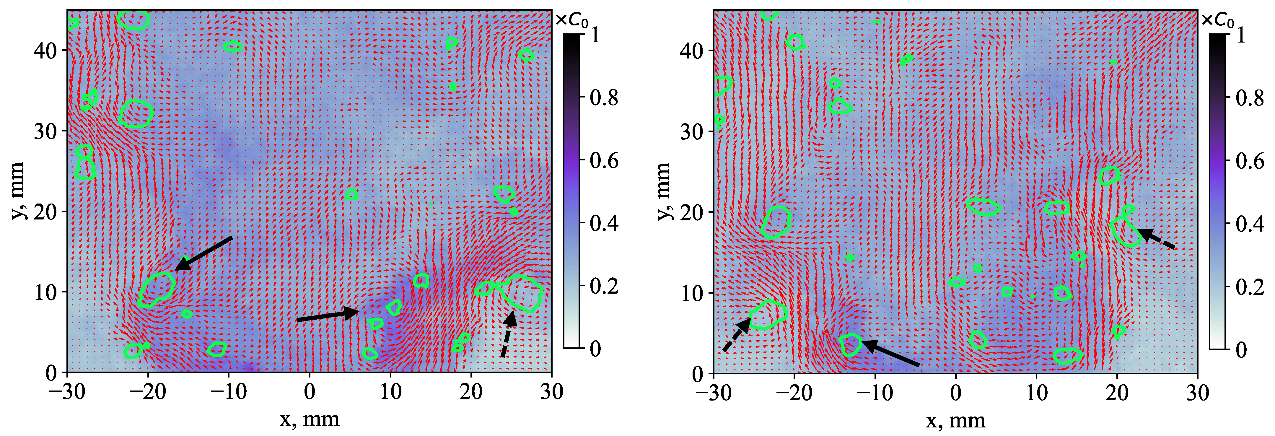
Figure 6.
Examples of the instantaneous flow velocity and model fuel concentration in x0y plane for the case of a 10% central jet injection.
Figure 6.
Examples of the instantaneous flow velocity and model fuel concentration in x0y plane for the case of a 10% central jet injection.
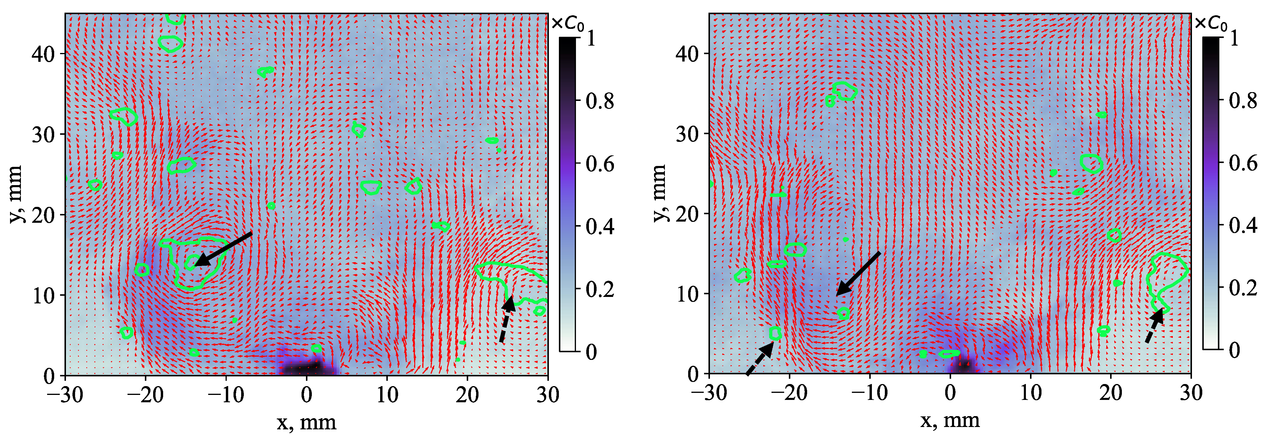
Figure 7.
Examples of the instantaneous flow velocity and model fuel concentration in x0y plane for the case of a 50% central jet injection.
Figure 7.
Examples of the instantaneous flow velocity and model fuel concentration in x0y plane for the case of a 50% central jet injection.

Figure 8.
Time-averaged velocity field and concentration fields for the cases: (a) without and (b) with a 50% central jet injection.
Figure 8.
Time-averaged velocity field and concentration fields for the cases: (a) without and (b) with a 50% central jet injection.
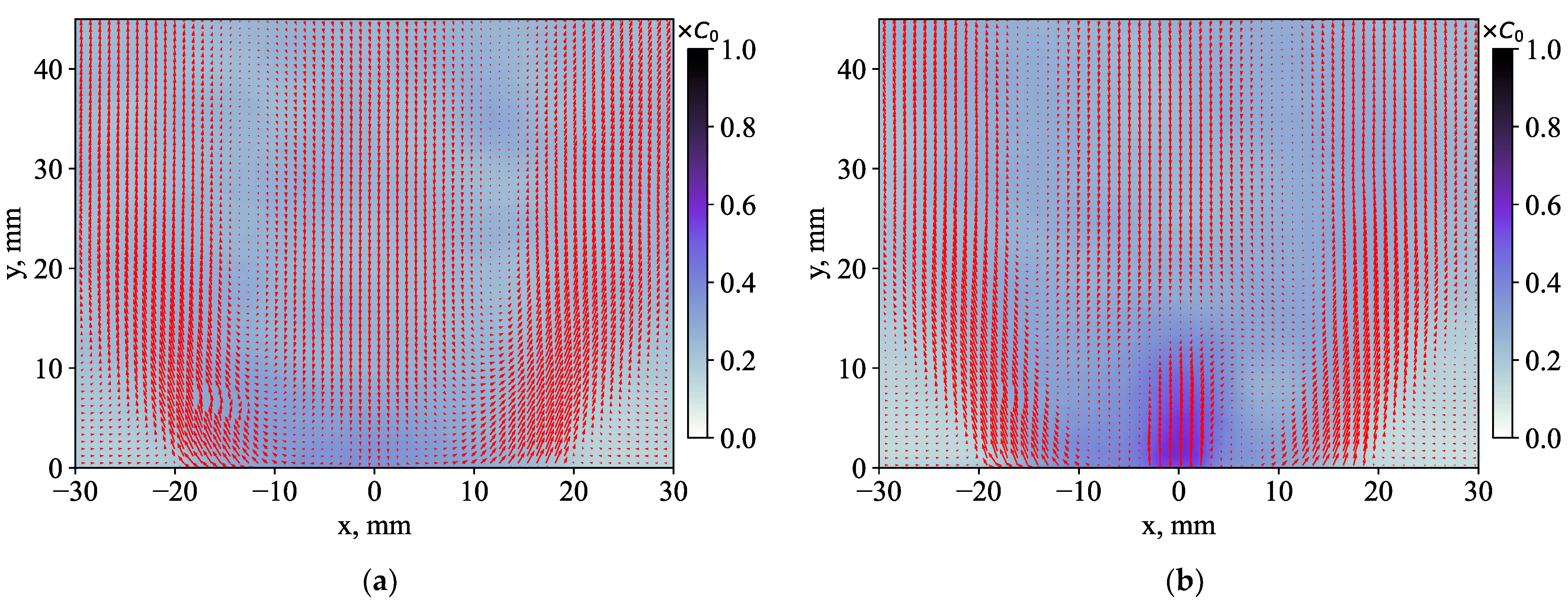
Figure 9.
Profiles of the time-averaged velocity components for the flow cross-section with y = 3.7 mm without and with a 10% and 50% central jet injection. (a) Longitudinal and (b) transversal components.
Figure 9.
Profiles of the time-averaged velocity components for the flow cross-section with y = 3.7 mm without and with a 10% and 50% central jet injection. (a) Longitudinal and (b) transversal components.
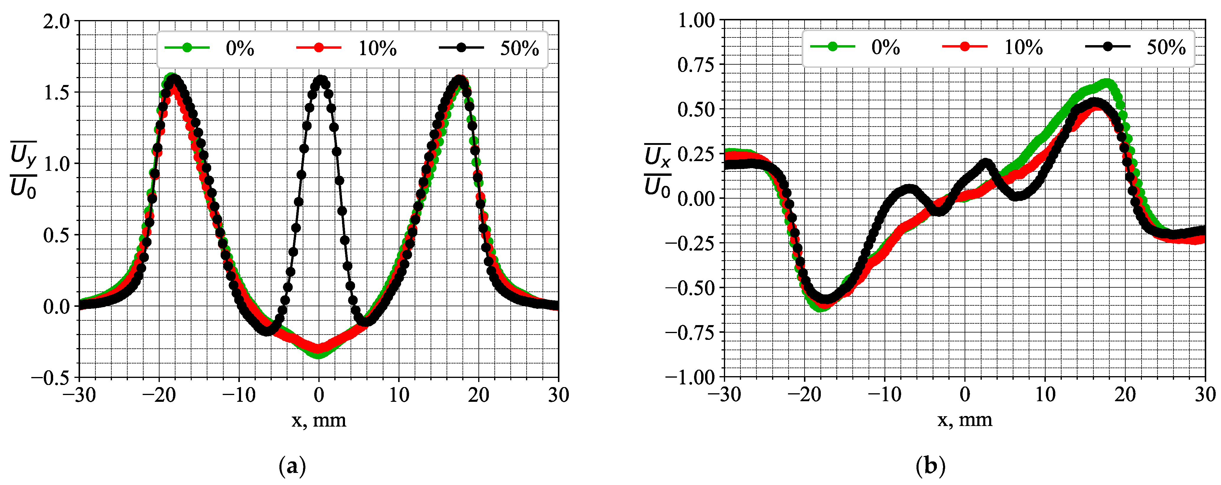
Figure 10.
Mean square deviation <ux′2> of the radial velocity fluctuations and the examples of local values for the cases: (a) without and (b) with a 50% central jet injection.
Figure 10.
Mean square deviation <ux′2> of the radial velocity fluctuations and the examples of local values for the cases: (a) without and (b) with a 50% central jet injection.
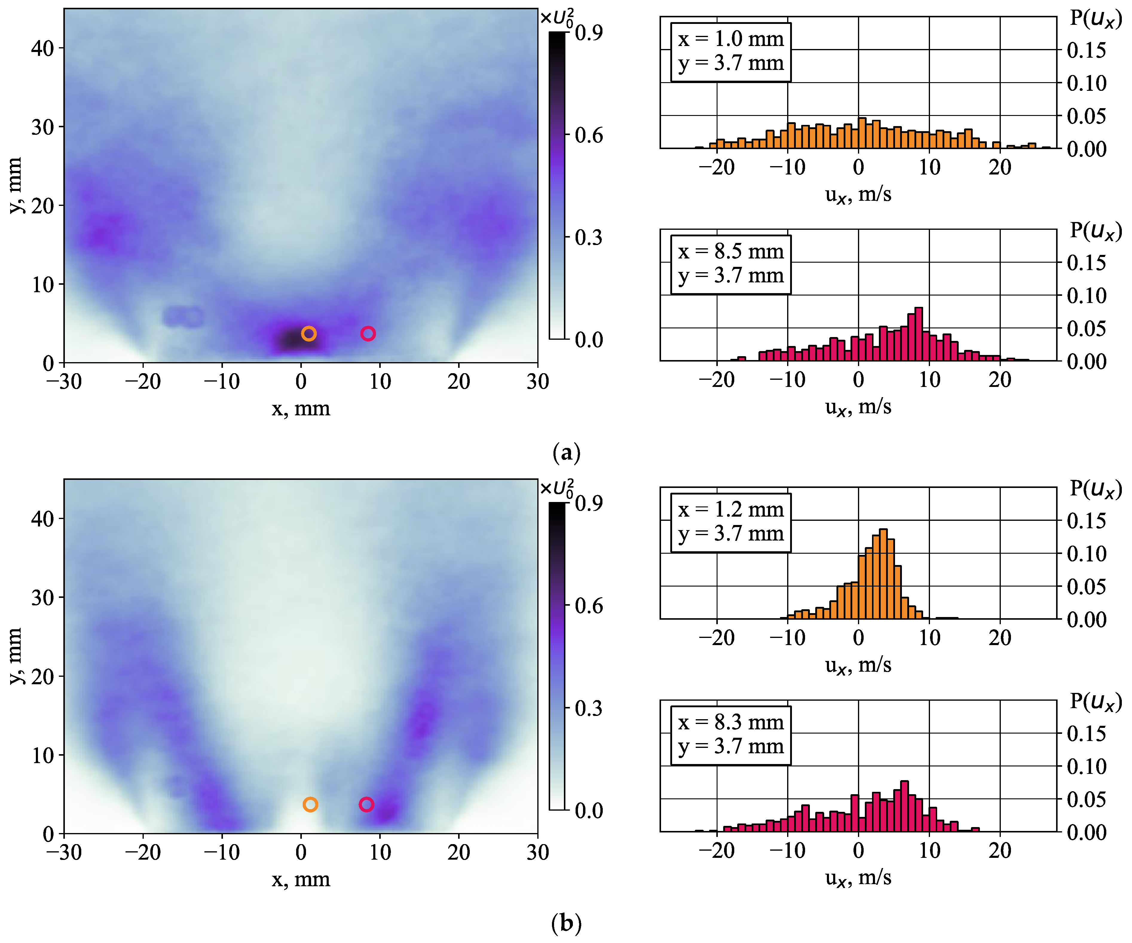
Figure 11.
Mean square deviation <uy′2> of the axial velocity fluctuations and the examples of local values for the cases: (a) without and (b) with a 50% central jet injection.
Figure 11.
Mean square deviation <uy′2> of the axial velocity fluctuations and the examples of local values for the cases: (a) without and (b) with a 50% central jet injection.
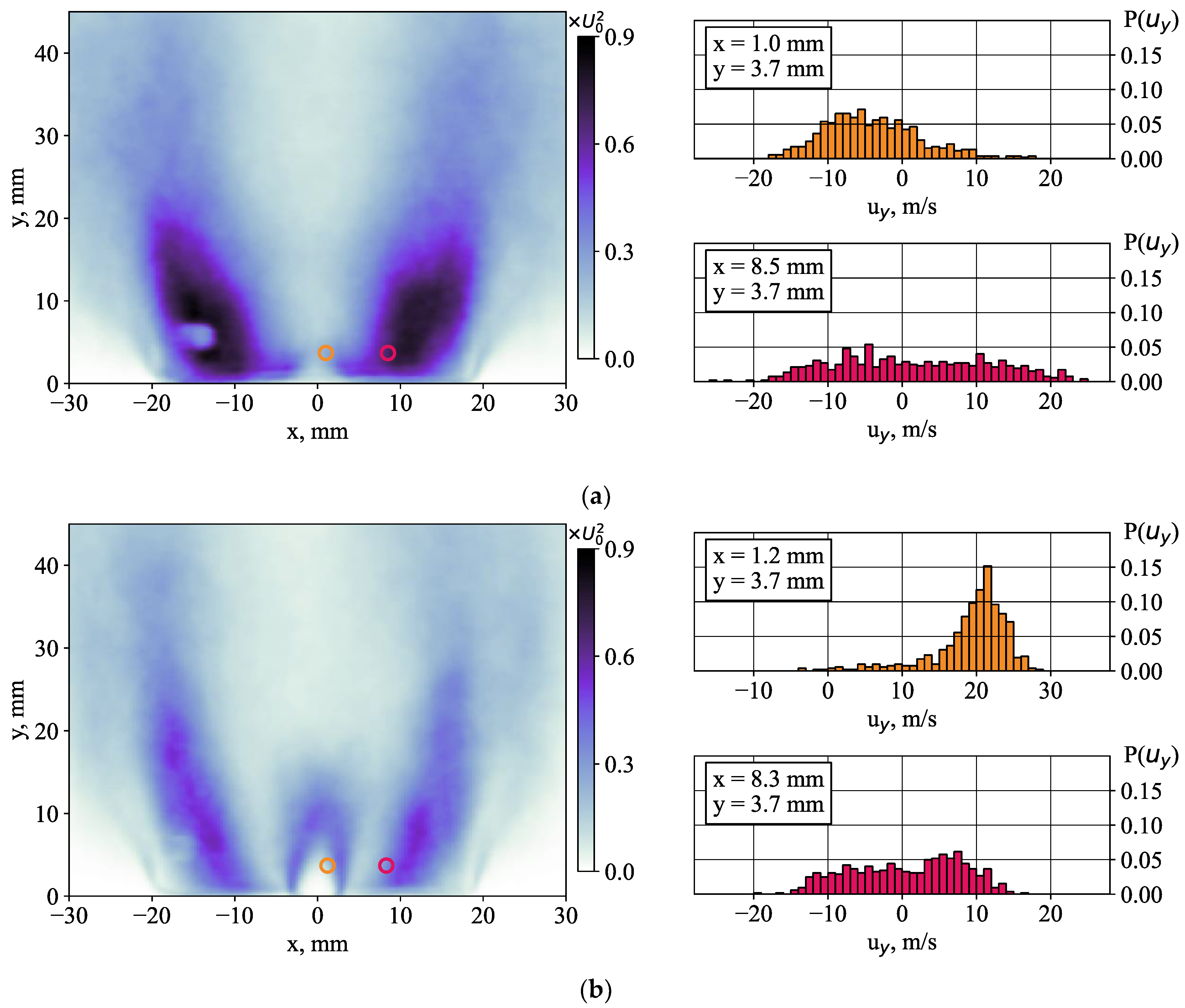
Figure 12.
Profiles of the intensities of velocity fluctuations for the flow cross-section with y = 3.7 mm without and with a 10% and 50% central jet injection. (a) Radial and (b) azimuthal velocity components.
Figure 12.
Profiles of the intensities of velocity fluctuations for the flow cross-section with y = 3.7 mm without and with a 10% and 50% central jet injection. (a) Radial and (b) azimuthal velocity components.
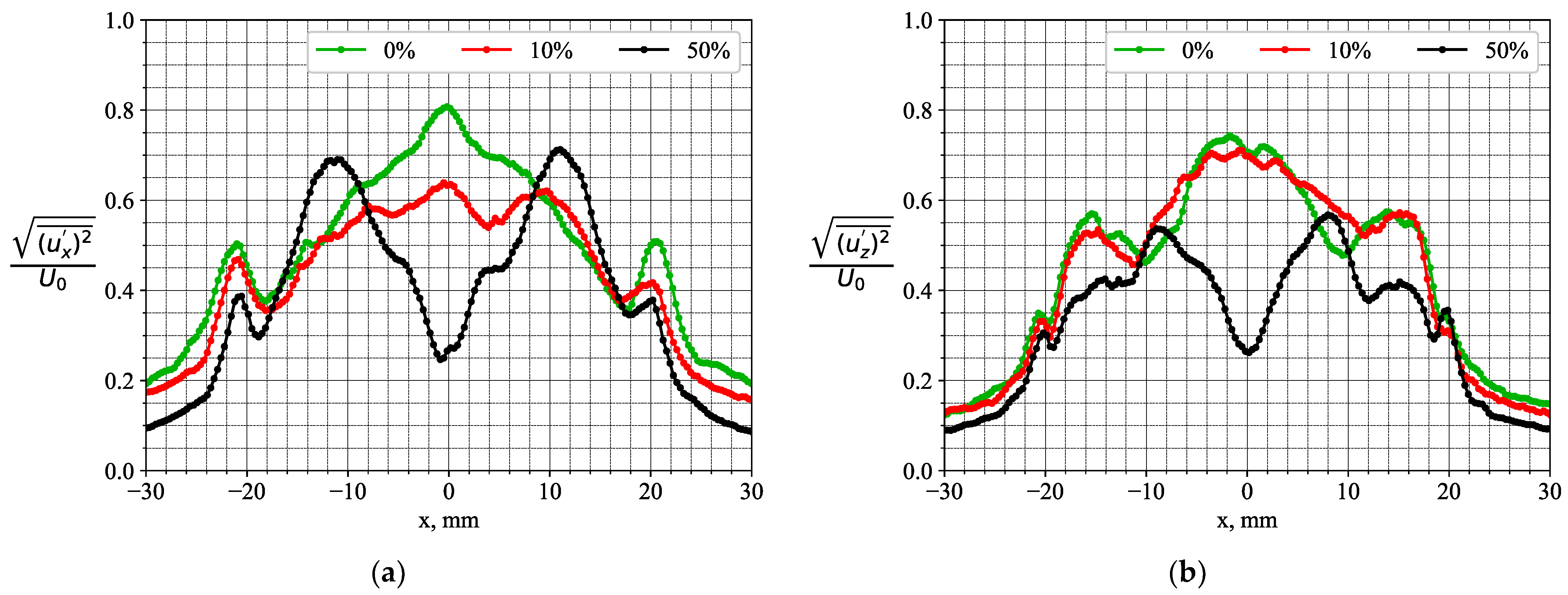
Figure 13.
Mean square deviation <c′2> of the acetone concentration and examples of local values for the cases: (a) without and (b) with a 50% central jet injection.
Figure 13.
Mean square deviation <c′2> of the acetone concentration and examples of local values for the cases: (a) without and (b) with a 50% central jet injection.

Figure 14.
(a) Distribution of kinetic energy of the velocity fluctuations associated with different POD modes and (b) temporal coefficients α1(t) and α2(t) for the cases of a 0%, 10% and 50% central jet injection.
Figure 14.
(a) Distribution of kinetic energy of the velocity fluctuations associated with different POD modes and (b) temporal coefficients α1(t) and α2(t) for the cases of a 0%, 10% and 50% central jet injection.

Figure 15.
Examples of (a) the first, (b) second, (c) third and (d) fourth POD modes and phase-averaged concentration fluctuations for the case without a central jet injection.
Figure 15.
Examples of (a) the first, (b) second, (c) third and (d) fourth POD modes and phase-averaged concentration fluctuations for the case without a central jet injection.
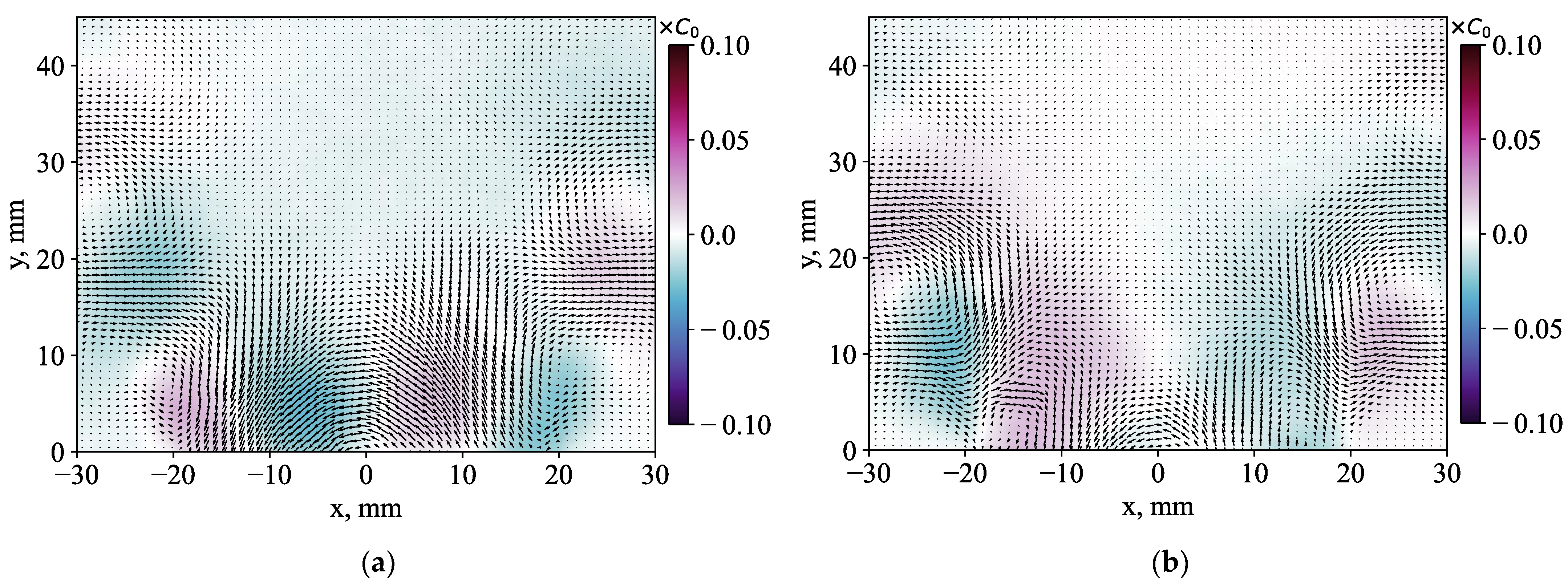
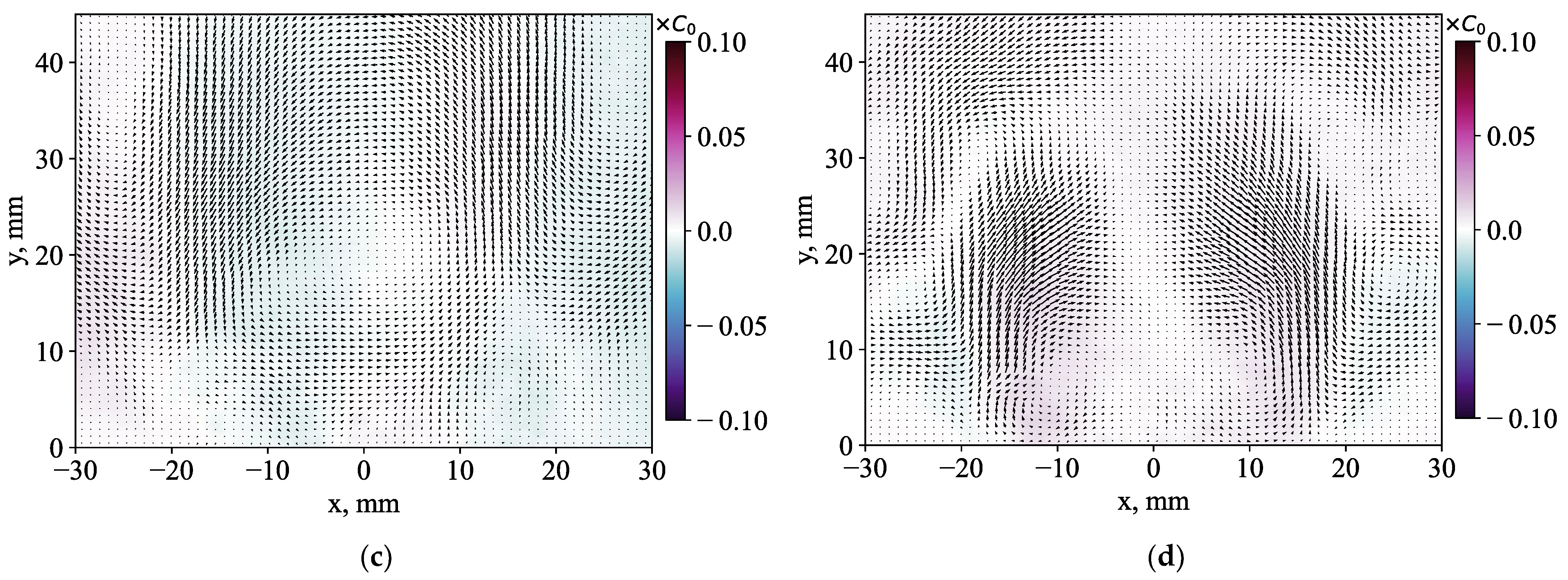
Figure 16.
Examples of (a) the first, (b) second, (c) third and (d) fourth POD modes and phase-averaged concentration fluctuations for the case of a 10% central jet injection.
Figure 16.
Examples of (a) the first, (b) second, (c) third and (d) fourth POD modes and phase-averaged concentration fluctuations for the case of a 10% central jet injection.
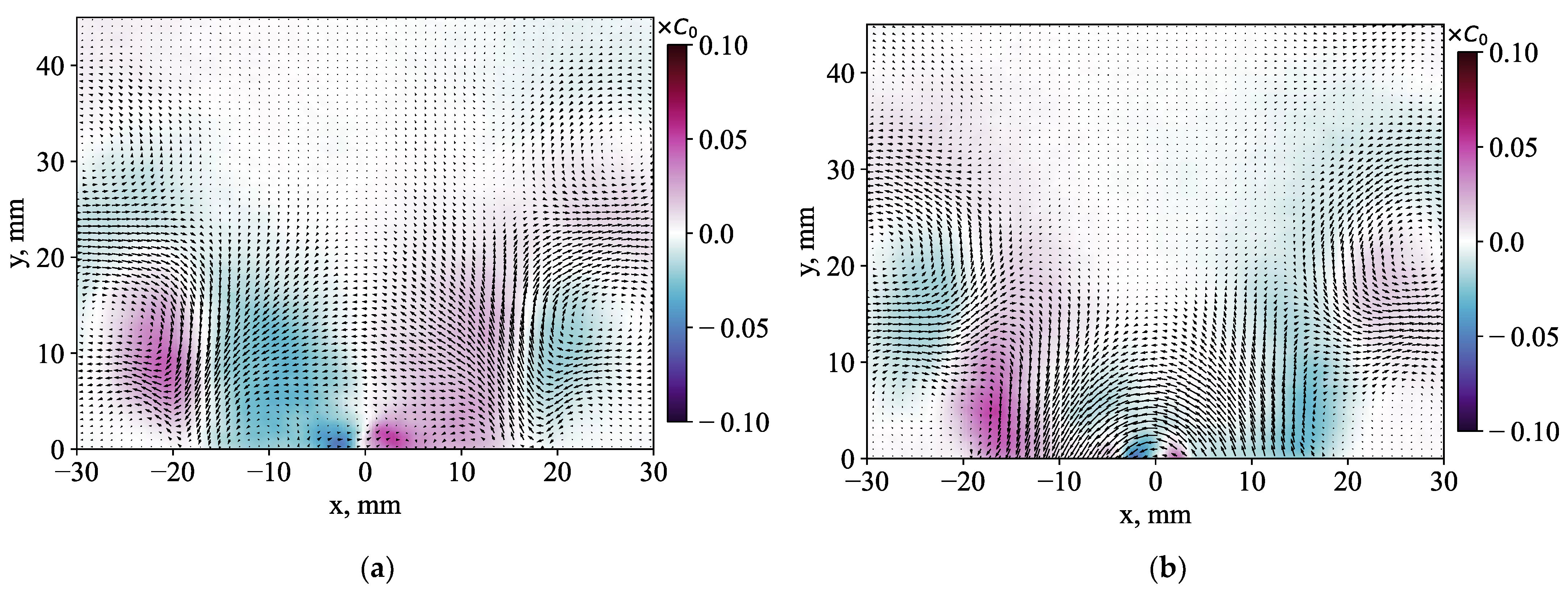

Figure 17.
Examples of (a) the first, (b) second, (c) third and (d) fourth POD modes and phase-averaged concentration fluctuations for the case of a 50% central jet injection.
Figure 17.
Examples of (a) the first, (b) second, (c) third and (d) fourth POD modes and phase-averaged concentration fluctuations for the case of a 50% central jet injection.
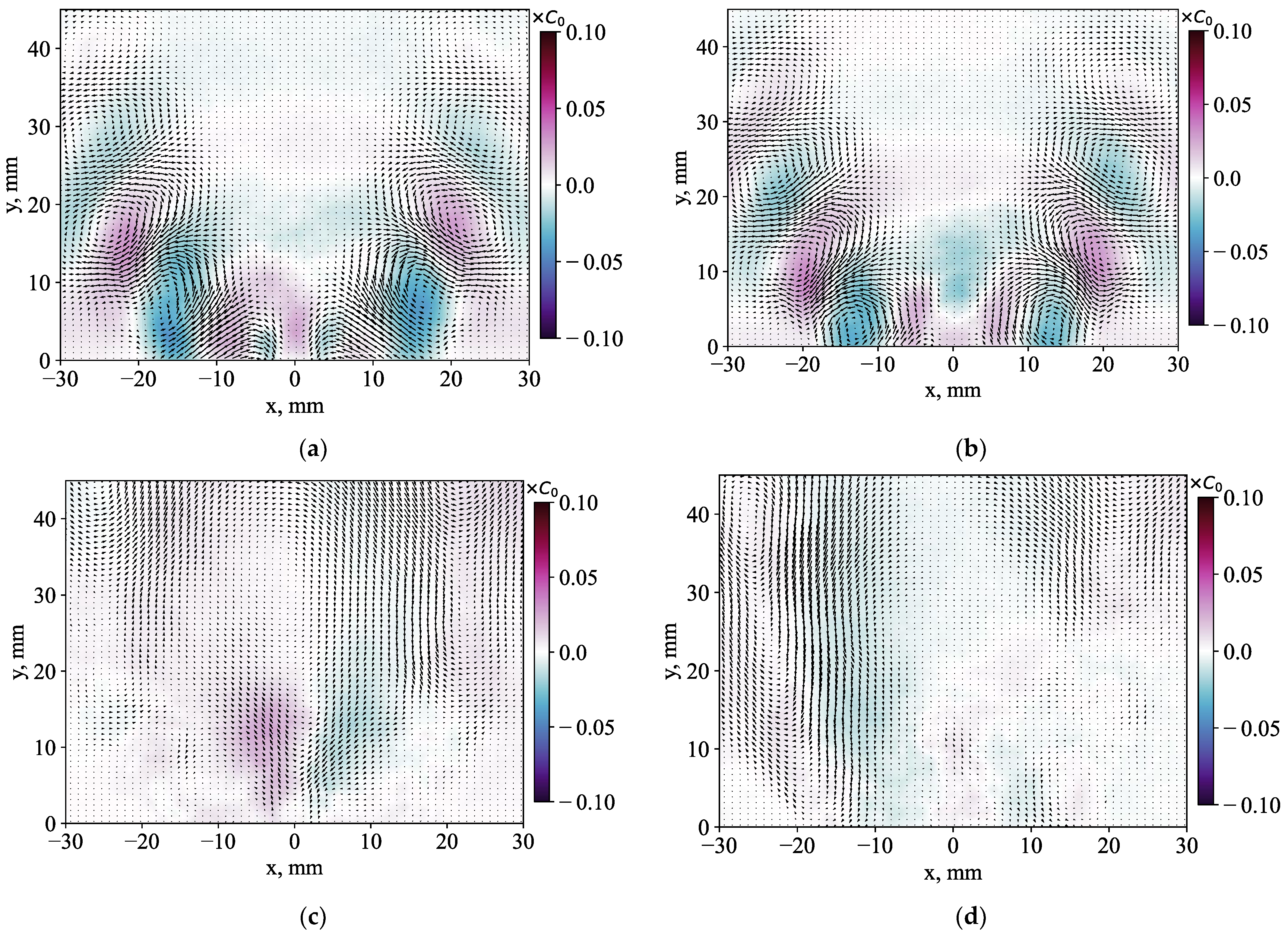
Figure 18.
Mean square deviation of the radial (a,c) <ux″2> and axial (b,d) <uy″2> components the stochastic velocity fluctuations for the cases: (a,b) without and (c,d) with a 50% central jet injection.
Figure 18.
Mean square deviation of the radial (a,c) <ux″2> and axial (b,d) <uy″2> components the stochastic velocity fluctuations for the cases: (a,b) without and (c,d) with a 50% central jet injection.


Figure 19.
Total (a,c) <ux′uy′> and stochastic (b,d) <ux″uy″> turbulent shear stress for the cases: (a,b) without and (c,d) with a 50% central jet injection.
Figure 19.
Total (a,c) <ux′uy′> and stochastic (b,d) <ux″uy″> turbulent shear stress for the cases: (a,b) without and (c,d) with a 50% central jet injection.
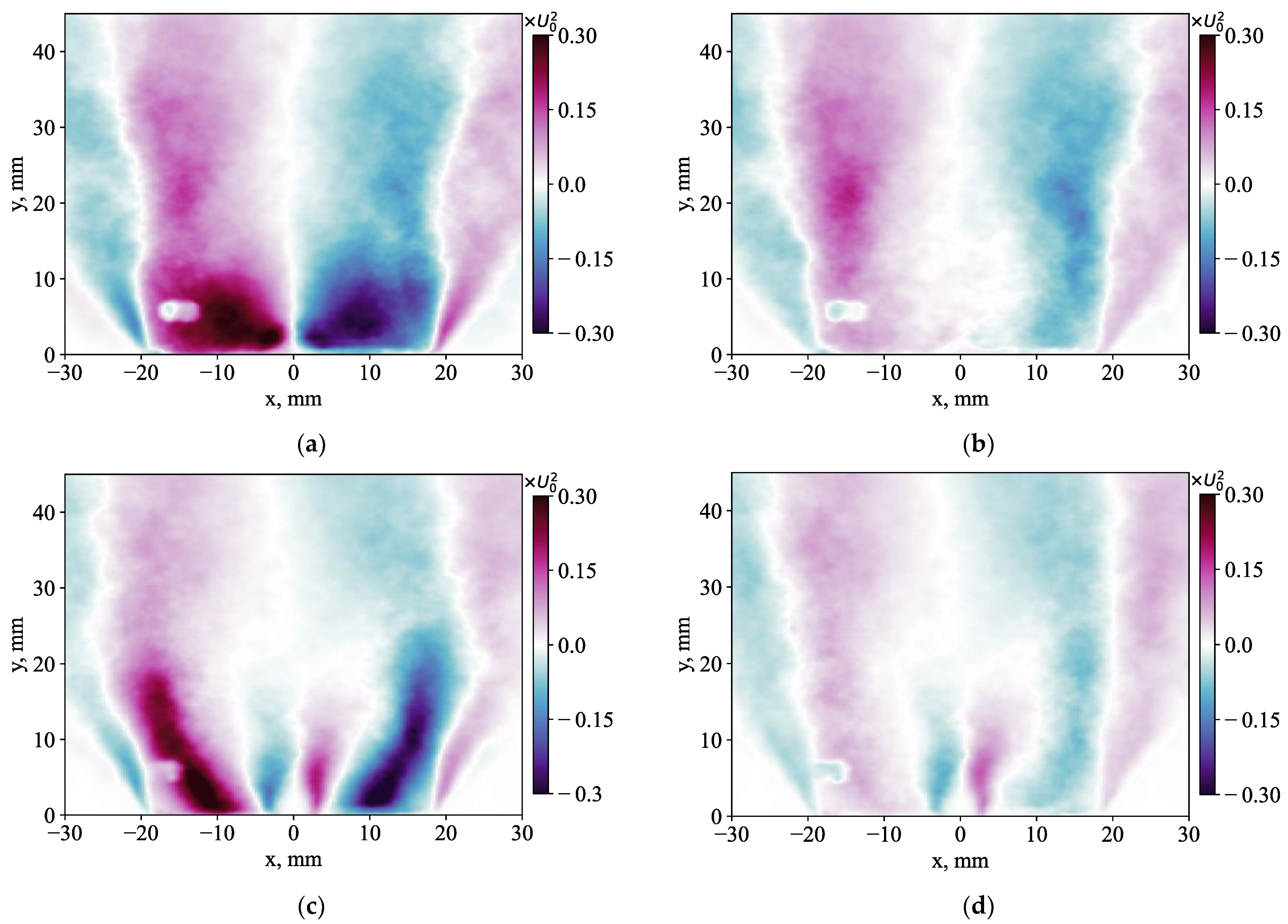
Figure 20.
Total (a,c) <ux′c′> and stochastic (b,d) <ux″c″> turbulent fluxes for the cases: (a,b) without and (c,d) with a 50% central jet injection.
Figure 20.
Total (a,c) <ux′c′> and stochastic (b,d) <ux″c″> turbulent fluxes for the cases: (a,b) without and (c,d) with a 50% central jet injection.

Figure 21.
The linearized anisotropy invariant maps for the cases: (a) without and (b) with a 50% central jet injection.
Figure 21.
The linearized anisotropy invariant maps for the cases: (a) without and (b) with a 50% central jet injection.

Table 1.
Flow parameters.
| Flowrate through Swirler (ln/min) | Flowrate between Vanes (ln/min) | Flowrate through Central Jet (ln/min) | Ratio through Central Jet |
|---|---|---|---|
| 799 | 58.3 | 0 | 0% |
| 799 | 52.5 | 5.8 | 10% |
| 799 | 29.15 | 29.15 | 50% |
Disclaimer/Publisher’s Note: The statements, opinions and data contained in all publications are solely those of the individual author(s) and contributor(s) and not of MDPI and/or the editor(s). MDPI and/or the editor(s) disclaim responsibility for any injury to people or property resulting from any ideas, methods, instructions or products referred to in the content. |
© 2023 by the authors. Licensee MDPI, Basel, Switzerland. This article is an open access article distributed under the terms and conditions of the Creative Commons Attribution (CC BY) license (https://creativecommons.org/licenses/by/4.0/).
Share and Cite
MDPI and ACS Style
Savitskii, A.; Sharaborin, D.; Chikishev, L.; Dulin, V. Flow Instability Control in a Model Swirl-Stabilized Combustor with Central Jet Injection. Inventions 2023, 8, 148. https://doi.org/10.3390/inventions8060148
AMA Style
Savitskii A, Sharaborin D, Chikishev L, Dulin V. Flow Instability Control in a Model Swirl-Stabilized Combustor with Central Jet Injection. Inventions. 2023; 8(6):148. https://doi.org/10.3390/inventions8060148
Chicago/Turabian StyleSavitskii, Alexey, Dmitriy Sharaborin, Leonid Chikishev, and Vladimir Dulin. 2023. "Flow Instability Control in a Model Swirl-Stabilized Combustor with Central Jet Injection" Inventions 8, no. 6: 148. https://doi.org/10.3390/inventions8060148