

Applications of the Order Reduction Optimization of the H-Infinity Controller in Smart Structures

 ,
,  and
and
Abstract
:1. Introduction
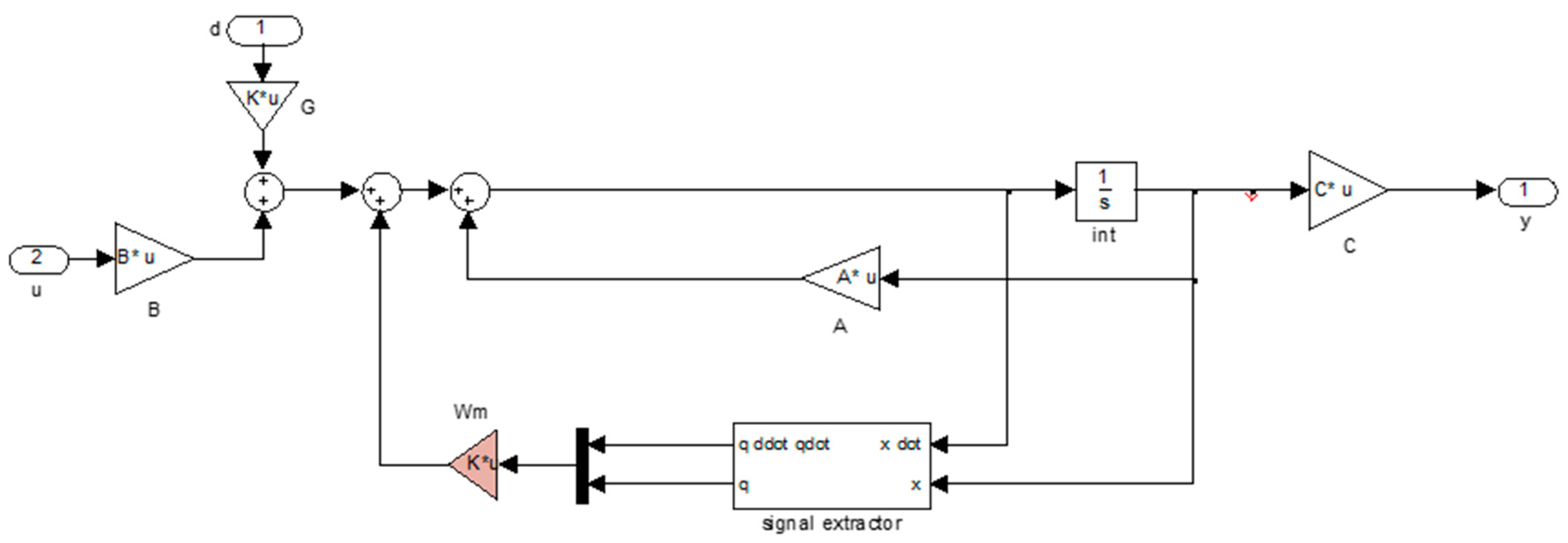
2. Methodology
2.1. Controller Synthesis H-Infinity
2.2. Optimization Method Hifoo
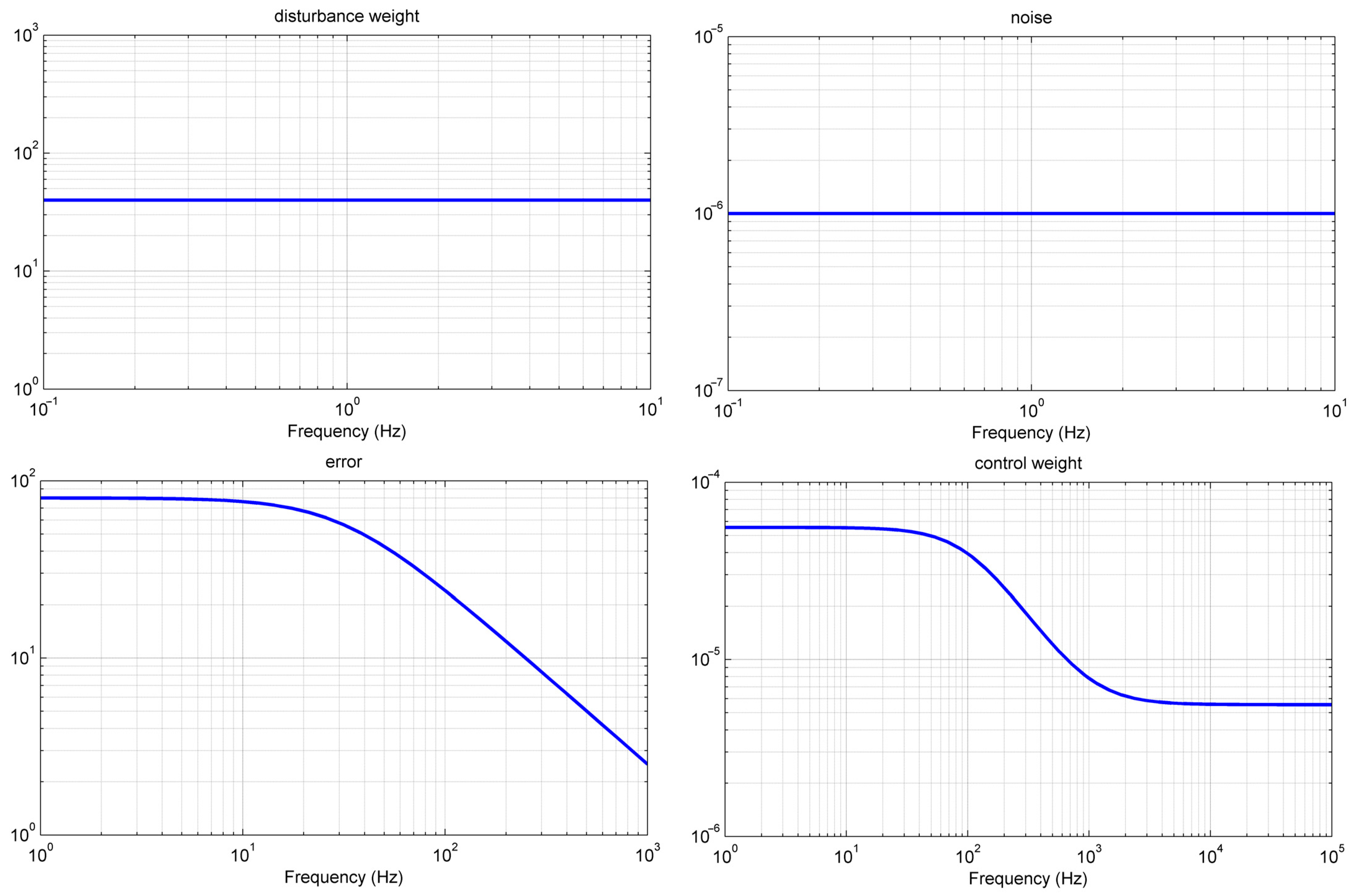
2.3. Problem Formulation and Optimization Method
K stabilizing
K stabilizing and K stable
3. Results
3.1. Application in Smart Structures
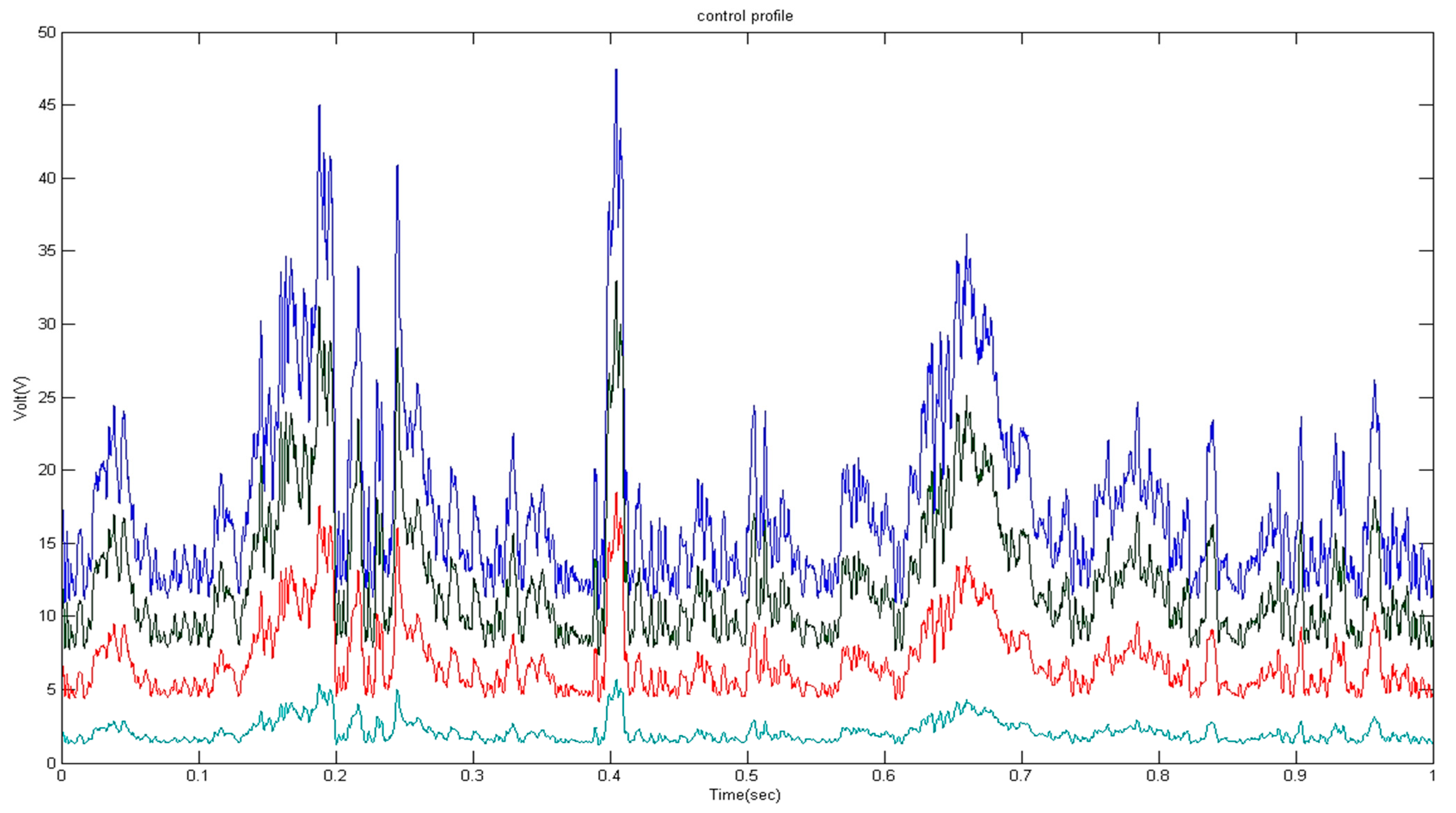
3.2. Results for H-Infinity Control
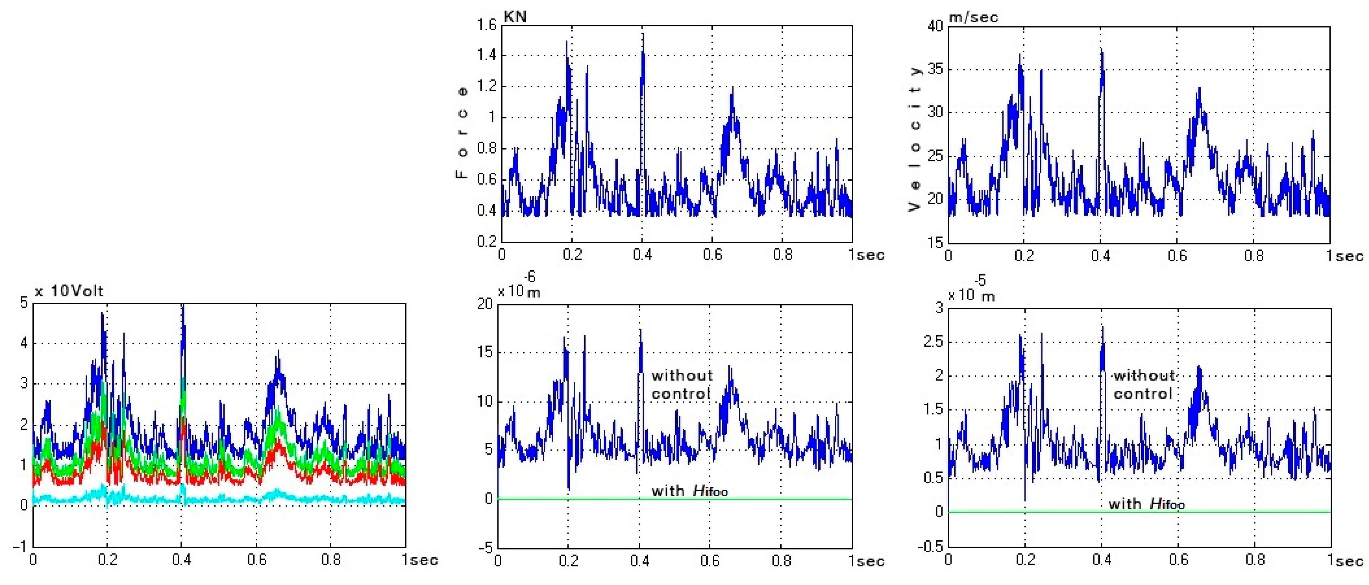
3.3. Results for Hifoo Control
4. Discussion
5. Conclusions
Author Contributions
Funding
Data Availability Statement
Acknowledgments
Conflicts of Interest
References
- Benjeddou, A.; Trindade, M.A.; Ohayon, R. New Shear Actuated Smart Structure Beam Finite Element. AIAA J. 1999, 37, 378–383. [Google Scholar] [CrossRef]
- Bona, B.; Indri, M.; Tornambe, A. Flexible Piezoelectric Structures-Approximate Motion Equations and Control Algorithms. IEEE Trans. Autom. Control 1997, 42, 94–101. [Google Scholar] [CrossRef]
- Okko, B.; Kwakernaak, H.; Gjerrit, M. Design Methods for Control Systems; Course Notes; Dutch Institute for Systems and Control: Delft, The Netherlands, 2001; Volume 67. [Google Scholar]
- Burke, J.V.; Henrion, D.; Lewis, A.S.; Overton, M.L. HIFOO—A matlab package for fixed-order controller design and H∞ optimization. IFAC Proc. Vol. 2006, 39, 339–344. [Google Scholar] [CrossRef]
- Burke, J.V.; Henrion, D.; Lewis, A.S.; Overton, M.L. Stabilization via Nonsmooth, Nonconvex Optimization. IEEE Trans. Autom. Control 2006, 51, 1760–1769. [Google Scholar] [CrossRef]
- Burke, J.V.; Lewis, A.S.; Overton, M.L. A Robust Gradient Sampling Algorithm for Nonsmooth, Nonconvex Optimization. SIAM J. Optim. 2005, 15, 751–779. [Google Scholar] [CrossRef]
- Burke, J.V.; Overton, M.L. Variational Analysis of Non-Lipschitz Spectral Functions. Math. Program. 2001, 90, 317–351. [Google Scholar] [CrossRef]
- Choi, S.-B.; Cheong, C.-C.; Lee, C.-H. Position Tracking Control of a Smart Flexible Structure Featuring a Piezofilm Actuator. J. Guid. Control Dyn. 1996, 19, 1364–1369. [Google Scholar] [CrossRef]
- Culshaw, B. Smart Structures—A Concept or a Reality? Proc. Inst. Mech. Eng. Part I J. Syst. Control Eng. 1992, 206, 1–8. [Google Scholar] [CrossRef]
- Doyle, J.; Glover, K.; Khargonekar, P.; Francis, B. State-Space Solutions to Standard H2 and H∞ Control Problems. In Proceedings of the 1988 American Control Conference, Atlanta, GA, USA, 15–17 June 1988; pp. 1691–1696. [Google Scholar]
- Tzou, H.S.; Gabbert, U. Structronics—A New Discipline and Its Challenging Issues. Fortschr.-Ber. VDI Smart Mech. Syst.—Adapt. Reihe 1997, 11, 245–250. [Google Scholar]
- Tzou, H.S.; Anderson, G.L. Intelligent Structural Systems; Springer: Dordrecht, The Netherlands; Boston, MA, USA; London, UK, 1992; ISBN 978-94-017-1903-2. [Google Scholar]
- Guran, A.; Tzou, H.-S.; Anderson, G.L.; Natori, M.; Gabbert, U.; Tani, J.; Breitbach, E. Structronic Systems: Smart Structures, Devices and Systems; World Scientific: Singapore, 1998; Volume 4, ISBN 978-981-02-2652-7. [Google Scholar]
- Gabbert, U.; Tzou, H.S. IUTAM Symposium on Smart Structures and Structronic Systems. In Proceedings of the IUTAM Symposium, Magdeburg, Germany, 26–29 September 2000; Kluwer: Dordrecht, The Netherlands; Boston, MA, USA; London, UK, 2001. [Google Scholar]
- Tzou, H.S.; Natori, M.C. Piezoelectric Materials and Continua; Braun, S., The Encyclopedia of Vibration, Eds.; Elsevier: Oxford, UK, 2001; pp. 1011–1018. ISBN 978-0-12-227085-7. [Google Scholar]
- Cady, W.G. Piezoelectricity: An Introduction to the Theory and Applications of Electromechanical Phenomena in Crystals; Dover Publication: New York, NY, USA, 1964. [Google Scholar]
- Tzou, H.S.; Bao, Y. A Theory on Anisotropic Piezothermoelastic Shell Laminates with Sensor/Actuator Applications. J. Sound Vib. 1995, 184, 453–473. [Google Scholar] [CrossRef]
- David, C.; Sagris, D.; Petousis, M.; Nasikas, N.K.; Moutsopoulou, A.; Sfakiotakis, E.; Mountakis, N.; Charou, C.; Vidakis, N. Operational Performance and Energy Efficiency of MEX 3D Printing with Polyamide 6 (PA6): Multi-Objective Optimization of Seven Control Settings Supported by L27 Robust Design. Appl. Sci. 2023, 13, 8819. [Google Scholar] [CrossRef]
- Moutsopoulou, A.; Stavroulakis, G.E.; Petousis, M.; Vidakis, N.; Pouliezos, A. Smart Structures Innovations Using Robust Control Methods. Appl. Mech. 2023, 4, 856–869. [Google Scholar] [CrossRef]
- Cen, S.; Soh, A.-K.; Long, Y.-Q.; Yao, Z.-H. A New 4-Node Quadrilateral FE Model with Variable Electrical Degrees of Freedom for the Analysis of Piezoelectric Laminated Composite Plates. Compos. Struct. 2002, 58, 583–599. [Google Scholar] [CrossRef]
- Packard, A.; Doyle, J.; Balas, G. Linear, Multivariable Robust Control With a μ Perspective. J. Dyn. Syst. Meas. Control 1993, 115, 426–438. [Google Scholar] [CrossRef]
- Kim, S.-W.; Boo, C.-J.; Kim, S.; Kim, H.-C. Stable Controller Design of MIMO Systems in Real Grassmann Space. Int. J. Control Autom. Syst. 2012, 10, 213–226. [Google Scholar] [CrossRef]
- Feng, Z.; Allen, R. Reduced Order H∞ Control of an Autonomous Underwater Vehicle. IFAC Proc. Vol. 2003, 36, 121–126. [Google Scholar] [CrossRef]
- Chandrashekhara, K.; Varadarajan, S. Adaptive Shape Control of Composite Beams with Piezoelectric Actuators. J. Intell. Mater. Syst. Struct. 1997, 8, 112–124. [Google Scholar] [CrossRef]
- Ackermann, J. Robust Control, The Parameter Space Approach; Springer: London, UK, 2002; ISBN 978-1-85233-514-4. [Google Scholar]
- Gao, H.; Lam, J.; Wang, C. Controller Reduction with Error Performance: Continuous- and Discrete-Time Cases. Int. J. Control 2006, 79, 604–616. [Google Scholar] [CrossRef]
- Yang, S.M.; Lee, Y.J. Optimization of Noncollocated Sensor/Actuator Location and Feedback Gain in Control Systems. Smart Mater. Struct. 1993, 2, 96. [Google Scholar] [CrossRef]
- Ramesh Kumar, K.; Narayanan, S. Active Vibration Control of Beams with Optimal Placement of Piezoelectric Sensor/Actuator Pairs. Smart Mater. Struct. 2008, 17, 55008. [Google Scholar] [CrossRef]
- Hanagud, S.; Obal, M.W.; Calise, A.J. Optimal Vibration Control by the Use of Piezoceramic Sensors and Actuators. J. Guid. Control Dyn. 1992, 15, 1199–1206. [Google Scholar] [CrossRef]
- Song, G.; Sethi, V.; Li, H.-N. Vibration Control of Civil Structures Using Piezoceramic Smart Materials: A Review. Eng. Struct. 2006, 28, 1513–1524. [Google Scholar] [CrossRef]
- Karatzas, I.; Lehoczky, J.P.; Shreve, S.E.; Xu, G.-L. Modeling, Control and Implementation of Smart Structures: A FEM-State Space Approach. Springer: London, UK, 1990; ISBN 9783540483939. [Google Scholar]
- Miara, B.; Stavroulakis, G.E.; Valente, V. Topics on Mathematics for Smart Systems. In Proceedings of the European Conference, Rome, Italy, 26–28 October 2006; World Scientific Publishing: Singapore, 2006. [Google Scholar]
- Moutsopoulou, A.; Stavroulakis, G.E.; Pouliezos, A.; Petousis, M.; Vidakis, N. Robust Control and Active Vibration Suppression in Dynamics of Smart Systems. Inventions 2023, 8, 47. [Google Scholar] [CrossRef]
- Leibfritz, F. COMPl e Ib: COnstrained Matrix-Optimization Problem Library—A Collection of Test Examples for Nonlinear Semidefinite Programs, Control System Design and Related Problems; Universität Trier: Trier, Germany, 2001; pp. 1–23. [Google Scholar]
- Wie, B.; Bernstein, D.S. Benchmark Problems for Robust Control Design. J. Guid. Control Dyn. 1992, 15, 1057–1059. [Google Scholar] [CrossRef]
- Burke, J.V.; Lewis, A.S.; Overton, M.L. A Nonsmooth, Nonconvex Optimization Approach to Robust Stabilization by Static Output Feedback and Low-Order Controllers. IFAC Proc. Vol. 2003, 36, 175–181. [Google Scholar] [CrossRef]
- Henrion, D.; Overton, M.L. Maximizing the Closed Loop Asymptotic Decay Rate for the Two-Mass-Spring Control Problem. arXiv 2006, arXiv:math/0603681. [Google Scholar]
- Henrion, D.; Sebek, M. Overcoming Non-Convexity in Polynomial Robust Control Design. In Proceedings of the Symposium on Mathematical Theory of Networks and Systems, Leuven, Belgium, 1 January 2004. [Google Scholar]
- Zhang, N.; Kirpitchenko, I. Modelling Dynamics of A Continuous Structure with a Piezoelectric Sensoractuator for Passive Structural Control. J. Sound Vib. 2002, 249, 251–261. [Google Scholar] [CrossRef]
- Vidakis, N.; Petousis, M.; Mountakis, N.; Moutsopoulou, A.; Karapidakis, E. Energy Consumption vs. Tensile Strength of Poly [ Methyl Methacrylate ] in Material Extrusion 3D Printing: The Impact of Six Control Settings. Polymers 2023, 15, 845. [Google Scholar] [CrossRef]
- Vidakis, N.; Petousis, M.; Mountakis, N.; Papadakis, V.; Moutsopoulou, A. Mechanical Strength Predictability of Full Factorial, Taguchi, and Box Behnken Designs: Optimization of Thermal Settings and Cellulose Nanofibers Content in PA12 for MEX AM. J. Mech. Behav. Biomed. Mater. 2023, 142, 105846. [Google Scholar] [CrossRef]
- Petousis, M.; Vidakis, N.; Mountakis, N.; Karapidakis, E.; Moutsopoulou, A. Functionality Versus Sustainability for PLA in MEX 3D Printing: The Impact of Generic Process Control Factors on Flexural Response and Energy Efficiency. Polymers 2023, 15, 1232. [Google Scholar] [CrossRef] [PubMed]
- Kwakernaak, H. Robust Control and H∞-Optimization—Tutorial Paper. Automatica 1993, 29, 255–273. [Google Scholar] [CrossRef]
- Blondel, V.D.; Tsitsiklis, J.N. A Survey of Computational Complexity Results in Systems and Control. Automatica 2000, 36, 1249–1274. [Google Scholar] [CrossRef]
- Zhang, X.; Shao, C.; Li, S.; Xu, D.; Erdman, A.G. Robust H∞ Vibration Control for Flexible Linkage Mechanism Systems With Piezoelectric Sensors And Actuators. J. Sound Vib. 2001, 243, 145–155. [Google Scholar] [CrossRef]
- Stavroulakis, G.E.; Foutsitzi, G.; Hadjigeorgiou, E.; Marinova, D.; Baniotopoulos, C.C. Design and Robust Optimal Control of Smart Beams with Application on Vibrations Suppression. Adv. Eng. Softw. 2005, 36, 806–813. [Google Scholar] [CrossRef]
- Kimura, H. Robust Stabilizability for a Class of Transfer Functions. IEEE Trans. Autom. Control 1984, 29, 788–793. [Google Scholar] [CrossRef]
- Francis, B.A. A Course in H∞ Control Theory; Springer: Berlin/Heidelberg, Germany, 1987; ISBN 978-3-540-17069-3. [Google Scholar]
- Crawley, E.F.; de Luis, J. Use of piezoelectric actuators as elements of intelligent structures. AIAA J. 1987, 25, 1373–1385. [Google Scholar] [CrossRef]
- Stavropoulos, P.; Chantzis, D.; Doukas, C.; Papacharalampopoulos, A.; Chryssolouris, G. Monitoring and Control of Manufacturing Processes: A Review. Procedia CIRP 2013, 8, 421–425. [Google Scholar] [CrossRef]
- Turchenko, V.A.; Trukhanov, S.V.; Kostishin, V.G.; Damay, F.; Porcher, F.; Klygach, D.S.; Vakhitov, M.G.; Lyakhov, D.; Michels, D.; Bozzo, B.; et al. Features of Structure, Magnetic State and Electrodynamic Performance of SrFe12−xInxO19. Sci. Rep. 2021, 11, 18342. [Google Scholar] [CrossRef]
- Almessiere, M.A.; Slimani, Y.; Algarou, N.A.; Vakhitov, M.G.; Klygach, D.S.; Baykal, A.; Zubar, T.I.; Trukhanov, S.V.; Trukhanov, A.V.; Attia, H.; et al. Tuning the Structure, Magnetic, and High Frequency Properties of Sc-Doped Sr0.5Ba0.5ScxFe12-XO19/NiFe2O4 Hard/Soft Nanocomposites. Adv. Electron. Mater. 2022, 8, 2101124. [Google Scholar] [CrossRef]
- Zaszczyńska, A.; Gradys, A.; Sajkiewicz, P. Progress in the applications of smart piezoelectric materials for medical devices. Polymers 2020, 12, 2754. [Google Scholar] [CrossRef]


| Parameters | Values |
|---|---|
| L, for beam length | 1.00 m |
| W, for Beam Width | 0.002 m |
| Wp, PZT Width | 0.002 m |
| h, for Beam thickness | 0.096 m |
| hp, piezoelectric thickness | 0.0002 m |
| ρ, for Beam density | 1600 kg/m3 |
| E, for Young’s modulus of the beam Ep, Young modulus of pzt 6.3 × 10¹⁰ N/m2 | 1.5 × 10¹¹ N/m2 |
| bs, ba, for PZT thickness | 0.002 m |
| d31 the Piezoelectric constant | 230 × 10−12 m/V |
Disclaimer/Publisher’s Note: The statements, opinions and data contained in all publications are solely those of the individual author(s) and contributor(s) and not of MDPI and/or the editor(s). MDPI and/or the editor(s) disclaim responsibility for any injury to people or property resulting from any ideas, methods, instructions or products referred to in the content. |
© 2023 by the authors. Licensee MDPI, Basel, Switzerland. This article is an open access article distributed under the terms and conditions of the Creative Commons Attribution (CC BY) license (https://creativecommons.org/licenses/by/4.0/).
Share and Cite
Moutsopoulou, A.; Petousis, M.; Vidakis, N.; Stavroulakis, G.E.; Pouliezos, A. Applications of the Order Reduction Optimization of the H-Infinity Controller in Smart Structures. Inventions 2023, 8, 150. https://doi.org/10.3390/inventions8060150
Moutsopoulou A, Petousis M, Vidakis N, Stavroulakis GE, Pouliezos A. Applications of the Order Reduction Optimization of the H-Infinity Controller in Smart Structures. Inventions. 2023; 8(6):150. https://doi.org/10.3390/inventions8060150
Chicago/Turabian StyleMoutsopoulou, Amalia, Markos Petousis, Nectarios Vidakis, Georgios E. Stavroulakis, and Anastasios Pouliezos. 2023. "Applications of the Order Reduction Optimization of the H-Infinity Controller in Smart Structures" Inventions 8, no. 6: 150. https://doi.org/10.3390/inventions8060150